Fairer Benchmarking of Optimization Algorithms ... - Optimization Online

Fairer Benchmarking of Optimization Algorithms via Derivative Free Optimization W. L. Hare∗

Y. Wang†

October 13, 2010

Abstract Research in optimization algorithm design is often accompanied by benchmarking a new algorithm. Some benchmarking is done as a proof-of-concept, by demonstrating the new algorithm works on a small number of difficult test problems. Alternately, some benchmarking is done in order to demonstrate that the new algorithm in someway out-performs previous methods. In this circumstance it is important to note that algorithm performance can heavily depend on the selection of a number of user inputed parameters. In this paper we begin by demonstrating that if algorithms are compared using arbitrary parameter selections, results do not just compare the algorithms, but also compare the authors’ ability to select good parameters. We further present a novel technique for generating and providing results using each algorithm’s “optimal parameter selection”. These optimal parameter selections can be computed using modern derivative free optimization methods and generate a framework for fairer benchmarking between optimization algorithms. Keywords: benchmarking, optimal parameter selection, Derivative Free Optimization

1

Introduction

Algorithm design is one of the pillars of modern optimization research. In order for a new algorithm to be considered successful, authors are generally encouraged to benchmark their algorithm against previously established methods. This consists of running several different algorithms against a collection of test problems and comparing the results. In this work, we examine an issue that arise during benchmarking and discuss a technique that can help researchers to provide fairer benchmarking of algorithms. In particular, we explore the question of how to avoid using arbitrary parameter selections during benchmarking. In [AO06], Audet and Orban point out that most optimization algorithms rely on a large quantity of input parameters that are independent of the optimization problem. For example, most optimization codes include a parameter how step length decreases as it is deemed too large. In this work we demonstrate that if algorithms are compared using arbitrary parameter selections, results do not just compare the algorithms, but also compare the authors’ ability to select good parameters. Thus it is unfair to compare two algorithms using arbitrary parameter selections. Working on the ideas of Audet and Orban, we suggest a novel methodology in which each algorithm’s “optimal parameter selection” is determined before benchmarking is performed. ∗ †

Dept of Math, Stats, & Physics, UBC O, [email protected]. Dept of App Math, UWO, [email protected].

1

In order to illustrate the ideas laid out in this work, we explore two methods of adapting the Nelder-Mead algorithm to include a very basic line search. It should be noted that the goal of this research is not to advance the Nelder-Mead algorithm. We select the Nelder-Mead algorithm for our illustrations for two reasons. First, despite criticisms on its effectiveness (see for example [McK99]), the Nelder-Mead algorithm is still one of the most widely applied optimization algorithms for applied problems [CSV09]. Second, as Nelder-Mead algorithm is not currently a major focus of active research, we are not biased to prove or disprove its effectiveness. The remainder of this paper is organized as follows. In Section 2 we outline the ideas behind optimal parameter selection, and outline the algorithms we shall use for our numerical examples. In Section 3 we discuss the test problems used in this paper, and review the construction and interpretation of performance profiles. In Section 4 we demonstrate that arbitrary parameter selections can result in inaccurate benchmarking of optimization algorithm. We then detail our method for determining the optimal parameter selections (Subsection 4.2) based on the work of Audet and Orban and argue that this parameter selection provides a fairer benchmark of the algorithms. We finish with some concluding remarks.

2

Overview and test algorithms

Considerable researcher into optimization focuses on the construction of computer implemented algorithms to solve minimization problems. Most algorithms include a variety of input parameters, to be chosen by the user, which represent aspects such as step-length reduction. With regards to these parameters, most algorithms can be proven to converge in a generally sense. That is, algorithms have some constraints on the parameter choice, but generally the number of options is continuous in nature. For example, a step-length reduction parameters might be required to be in τ ∈ (0, 1), but it is left to the user to determine whether to be aggressive (e.g., τ = 0.01), neutral (e.g., τ = 0.5), or conservative (e.g., τ = 0.95). From a purely theoretical point of view, this is a very powerful aspect of optimization research. However, from a practical point of view, this generates some difficulty when benchmarking algorithms. The benchmarking process consists of running several different algorithms against a collection of test problems and comparing the results. In benchmarking an algorithm, authors pursue one of two goals. In some benchmarking research, the goal is to show a proof-of-concept that the algorithm can be implemented and work in practice. For this goal, it suffices to select any parameter selection that results in reasonable performance. In other benchmarking research, the goal is to show that the new algorithm in someway out-performs previous methods. For this goal, the choice of parameters can be crucial. We shall see, in Section 4 Subsection 4.1, that small changes in algorithm parameters can vastly alter an algorithm’s performance. This leads naturally to the question of how to find good parameter selections for benchmarking, and how to find fair parameter selections for all algorithms. One option lies in recent results by Audet and Orban involving Derivative Free Optimization [AO06]. Derivative Free Optimization (DFO) methods are designed to minimize objective functions for which derivative information is not available. (We refer readers to the book of Conn, Scheinberg, and Vicente for general information on DFO methods [CSV09].) In [AO06], Audet and Orban demonstrate that parameter selection can be phrased as a DFO problem where the inputs are the parameters and the goal is to minimize run time. Of course, in order to apply this idea it is necessary to solve each optimization problem multiple times. In applied research this appears impractical, however Audet and Orban demonstrate how the use of a collection of surrogate functions (functions that are small versions of the original problem and maintain similar problem structure) can lead to a good parameter selection for the original problem.

2

In the case of benchmarking, the issue of solving the collection of test problems multiple times is not serious. Indeed, many researchers will attest that they “tinker” with algorithm parameters before benchmarking in order to attain better results. In this paper we propose that instead of “tinkering”, researchers apply the techniques of Audet and Orban to formally find the “optimal parameter selection” for each algorithm being benchmarked, and then compare algorithms under their optimal performance. In this paper we will utilize the classic Nelder-Mead algorithm and two simple variations in order to demonstrate the necessity of proper benchmarking techniques. For the sake of completeness, our implementation of the Nelder-Mead algorithm and details on our two variants are discussed in the remainder of this Section. All algorithms were implemented in MATLAB 7.6.0 (R2008a).

2.1

Classic Nelder-Mead (CNM)

One of the oldest methods in DFO literature is the famous Nelder-Mead algorithm [NM65]. Due to its ease in implementation, range of applications, and general effectiveness, the Nelder-Mead algorithm is still one of the most widely applied optimization algorithms [CSV09, Chpt 8]. The Nelder-Mead algorithm begins with a simplex of potential solution points to an optimization problem. After evaluating the objective function at each point, the algorithm operates a reflection, an expansion, a contraction (inside or outside) or a shrink on the simplex. The goal is to replace the current worst point of the simplex with a newly generated better point (if there is any) in order to have a potentially better pool of possible solutions. If no better point can be found, the shrink operation reduces the search area so a more precise local solution can be determined. A pseudo-code version of the Nelder-Mead algorithm appears in Algorithm 2.1. Algorithm 2.1 (Classic Nelder-Mead Algorithm: CNM) 0. Initialization: Input an initial simplex SP = {x0 , x1 , x2 , ..xn }, a reflection parameter 0 < α, an expansion parameter 1 < γ, a contraction parameter 0 < β < 1, a shrink parameter 0 < δ < 1, and stopping criteria. 1. Order: Determine the simplex points xb , xs , and xw such that their function values f b = f (xb ), f s = f (xs ), and f w = f (xw ) are a best, a second worst, and a worst. 2. Stopping: Check stopping criteria and terminate if desired. 3. Reflect: Compute the reflection point and value xr = c + α(c − xw ), f r = f (xr ) where c =

1 n

X xi ∈SP \xw

If f b ≤ f r < f s replace xw with xr and return to Order. If f r < f b proceed to Expand. Otherwise (f r ≥ f s ) proceed to Contract. 4. Expand: (f r < f b ) Compute the expansion point and value xe = c + γ(c − xw ), f e = f (xe ). If f e < f r replace xw with xe and return to Order. Otherwise replace xw with xr and return to Order. 5. Contract: (f r ≥ f s ) If f s ≤ f r < f w then compute the outside contraction point and value xc = c + β(c − xw ), f c = f (xc ).

3

xi .

If f c ≤ f r replace xw with xc and return to Order, Otherwise continue to Shrink. If f w ≤ f r then compute the inside contraction point and value xc = c + β(xw − c), f c = f (xc ). If f c < f w replace xw with xc and return to Order, Otherwise continue to Shrink. 6. Shrink: Reconstruct the simplex by setting xi = xb + δ(xi − xb ), for i = 0, 1, 2, ...n. Return to Order. Various implementations of Nelder-Mead have arisen in the past 40 years, each of which differs slightly from the original Nelder-Mead algorithm. Our implementation differs from the original in several manners. Most importantly, [NM65] does not consider the shrink parameter δ as a parameter, instead defining it to be 0.5. We also differ from [NM65] in a variety of small changes. For example, we accept the reflection point when f b ≤ f r < f s , while [NM65] accepted the reflection point when f b ≤ f r ≤ f s . Other changes of the same magnitude are also present. Most varieties of the Nelder-Mead algorithm differ from the [NM65] to a similar level (compare [NM65], [McK99], and [CSV09] for example). In Step 0, Initialization, we are required to input a starting simplex. However, most test problems, in particular those in [MGH81], provide a single starting point x0 ∈ IRn . One simple way of generating a starting simplex from a single point is to generate xi = x0 + ei for i = 1, 2, ...n, where {ei }ni=1 is an orthogonal set of unit direction vectors. We use this method, with the standard set of orthogonal unit vectors (ei contains a 1 in the ith position and 0 elsewhere). In Step 1, Order, we use the term “a” worst point (second worst, best) as it is possible that a tie may occur. In our implementation, points just added to the simplex are favoured over points that were previously in the simplex. Further ties (as could occur after a Shrink step) are broken by favouring the point with the lowest index. In Step 2, Stopping, we employ three stopping criteria. First, we stop as soon as more than 6000 function evaluations are detected (note this may result in slightly over 6000 function evaluations if, for example, a shrink step occurs at the final iteration). This ensures eventual stoppage regardless of the test problem. Second, we check the diameter of the simplex and terminate if the simplex becomes too small (< 10−6 ). Finally, we examine simplex degeneracy by implementing the simplex degeneracy test found in [CSV09] (with tolerance of 10−12 ).

2.2

Double Expansion Nelder-Mead (DENM)

In Step 4, Expand, the reflection point has demonstrated objective function improvement over the current best point. This effectively demonstrates that c − xw is a descent direction from the point xw . The expansion step allows the Nelder-Mead algorithm to explore further in that direction to a limited distance. In our first variant on the Nelder-Mead algorithm, we allow for a second expansion step when the first expansion point is successful. Algorithm 2.2 (Double Expansion Nelder-Mead: DENM) Replace Step 4 in Algorithm 2.1 with

4

4. Expand (DENM): (f r < f b ) Compute the expansion point and value xe = c + γ(c − xw ), f e = f (xe ). If f e ≥ f r then replace xw with xr and return to Order. Otherwise (f e < f r ), compute the second expansion point xe2 = c + γ(γ(c − xw )) and continue to 4b. 4b. Expand II: If (SP \ xw ) ∪ xe2 is nondegenerate then compute the second expansion value f e2 = f (xe2 ). Otherwise set f e2 = ∞. If f e2 < f e then replace xw with xe2 and return to Order. Otherwise (f e2 ≥ f e , f e < f r ) replace xw with xe and return to Order. In DENM the second expansion point is only adopted if the resulting geometry is nondegenerate and the function value at this new point is improved. This helps prevent the simplex from becoming degenerate too quickly. We perform a check on the new simplex geometric before evaluating the function at the second expansion point in order to avoid unnecessary function evaluations. As in the full algorithm, in Step 4b we implement the simplex degeneracy test from [CSV09] (with tolerance of 10−12 ).

2.3

Double Expansion Double Contraction Nelder-Mead (DEDCNM)

This variant is similar to DENM, however, we allow double contraction in additional to double expansion. Algorithm 2.3 (Double Expansion Double Contraction Nelder-Mead: DEDCNM) Replace Step 4 in Algorithm 2.1 with Step 4 of DENM (Algorithm 2.2). Replace Step 5 in Algorithm 2.1 with 5. Contract: (f r ≥ f s ) If f s ≤ f r < f w then compute the outside contraction point and value xc = c + β(c − xw ), f c = f (xc ). If f c > f r continue to Shrink Otherwise (f c ≤ f r ), compute the second outside contraction point xc2 = c + β(β(c − xw )) and continue to 5b If f w ≤ f r then compute the inside contraction point and value xc = c + β(xw − c), f c = f (xc ). If f c ≥ f w continue to Shrink Otherwise (f c < f w ), compute the second inside contraction point xc2 = c + β(β(xw − c))

5

and continue to 5b 5b. Contract II: If (SP \ xw ) ∪ xc2 is nondegenerate then compute the second contraction value f c2 = f (xc2 ). Otherwise set f c2 = ∞. If f c2 < f c then replace xw with xc2 and return to Order. Otherwise replace xw with xc and return to Order. Similar to DENM, the second expansion or the second contraction point is only adopted if the resulting geometry is nondegenerate and the function value at the new point is improved.

3

Test Problems and Performance Profiles

For our tests we use the problems listed in [MGH81]1 . In [MGH81], test problems are listed with a dimension (number of input variables) and a number of sub-functions; or a range of possible dimensions and number of sub-functions. Sub-functions describe the complexity of the problem Pm within a fixed dimension. In particular, each test problem is given of the form i=1 (fi )2 , where m is the number of sub-functions. The problems examined are listed in Table 1, Appendix A, along with the dimension and number of sub-functions each uses. Problem number is used for referencing, and refers to the problem number as provided in [MGH81]. In some cases, the problem listed in [MGH81] has options on the dimension or number of sub-functions. In such cases we report the numbers that we used. For further details on these test problems we refer readers to [MGH81]. In order to provide a visual comparison of each algorithms performance, we employ performance profiles as follows. Let tp,s represent the number of function evaluations required by solver s to solve problem p. If the solver fails to solve the problem then tp,s is set to infinity. From the values tp,s we generate the performance ratio value rp,s =

tp,s mins {tp,s }

for each solver and each problem. Performance profiles now graphs for each solver the function ρs (τ ) defined by 1 ρs (τ ) = {p : rp,s ≤ τ } , P where P is the number of test problem and |{·}| is the number of elements in the set {·}. Thus ρs (τ ) “is the probability for solver s that a performance ratio rp,s is within a factor τ ∈ IR of the best possible ratio” [DM02]. At the far left of the graphs (τ = 1) each solver begins at the value equal to the portion of test problems that it solved with the least number of function evaluations. At the far right (τ → ∞) each solver converges to the portion of test problems that it successfully solved. In general solver s1 is performing better than s2 if its graph is higher (i.e. ρs1 (τ ) > ρs2 (τ ) for most τ ).

4

Optimal parameters selections

The purpose of this paper is to demonstrate that benchmarking optimization algorithms using arbitrary parameter selections can create inconsistent results, and to suggest a simple solution 1

Some erratums to the [MGH81] problem list can be found at [KK97]. We implement these as appropriate.

6

to this problem. To demonstrate the flaw with arbitrary parameter selections, we compare CNM to the two variant describe in Subsections 2.2 and 2.3 using several different selections for the parameters α, γ, β, and δ. Stopping criteria, discussed in Subsection 2.1, are consistent across algorithms, and tuned to stop when the algorithm believes it has correctly determined the solution to 6 digits of accuracy. A problem is considered solved if the relative error, defined by |f min − f ∗ | RE := , (1) |f ∗ | + 1 where f min is the found minimum and f ∗ is the true global minimum, is less than 10−6 .

4.1

Comparisons Across Arbitrary Parameter Selections

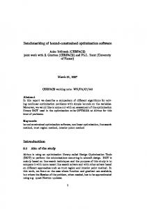
In the next three examples we show that CNM can perform worse than, similar to, or better than DENM, simply by considering different parameter selections. Example 4.1 (CNM is worse than DENM (α = 1, γ = 1.9, β = 0.6, and δ = 0.6)) We benchmark CNM and DENM using the parameter selection α = 1, γ = 1.9, β = 0.6, and δ = 0.6 (for both algorithms). Complete test results can be found in Table 2, Appendix A. In Figure 1 we provide the performance profile for this test. CNM versus DENM 1

P(( τp,s / min { tp,s: 1≤ s≤ ns} ) ≤ τ )

0.9 0.8 0.7 0.6 0.5 0.4 0.3 0.2 0.1 0

CNM DENM 1

1.2

1.4

1.6

τ

1.8

2

2.2

Figure 1: Performance profile of Classic Nelder-Mead versus Double Expansion Nelder-Mead using α = 1, γ = 1.9, β = 0.6, and δ = 0.6. Examining Figure 1 we see that the graph of CNM is never above the graph of DENM, so overall the performance profile suggests that CNM is worse than DENM. Example 4.2 (CNM and DENM are similar (α = 1, γ = 1.9, β = 0.5, and δ = 0.6)) We benchmark CNM and DENM using the parameter selection α = 1, γ = 1.9, β = 0.5, and δ = 0.6. Complete test results can be found in Table 3, Appendix A. In Figure 2 we provide the performance profile for this test. Examining Figure 2 we see that CNM begins above DENM, but ends below. The two graphs cross at about τ = 1.4. The performance profile suggests that DENM is slightly more robust than CNM, but slightly worse in speed. Overall the two algorithms are quite comparable. Example 4.3 (CNM is better than DENM (α = 1, γ = 2, β = 0.5, and δ = 0.5)) We benchmark CNM and DENM using the parameter selection α = 1, γ = 2, β = 0.5, and δ = 0.5. Complete test results can be found in Table 4, Appendix A. In Figure 3 we provide the performance profile for this test. Since the graph of CNM is above the graph of DENM at all times, the performance profile suggests that CNM is better than DENM.

7

CNM versus DENM 1

P(( τp,s / min { tp,s: 1≤ s≤ ns} ) ≤ τ )

0.9 0.8 0.7 0.6 0.5 0.4 0.3 0.2 0.1 0

CNM DENM 1

1.2

1.4

1.6

τ

1.8

2

2.2

Figure 2: Performance profile of Classic Nelder-Mead versus Double Expansion Nelder-Mead using α = 1, γ = 1.9, β = 0.5, and δ = 0.6. CNM versus DENM 1

P(( τp,s / min { tp,s: 1≤ s≤ ns} ) ≤ τ )

0.9 0.8 0.7 0.6 0.5 0.4 0.3 0.2 0.1 0

CNM DENM 1

1.2

1.4

1.6

τ

1.8

2

2.2

Figure 3: Performance profile of Classic Nelder-Mead versus Double Expansion Nelder-Mead using α = 1, γ = 2, β = 0.5, and δ = 0.5.

Our next example quickly shows that the same inconsistency of results can be achieved for DEDCNM. Example 4.4 (comparing CNM and DEDCNM) We benchmark CNM and DEDCNM using three parameter selections: i) α = 1.1, γ = 2, β = 0.8, and δ = 0.5, i) α = 1, γ = 2, β = 0.7, and δ = 0.5, and i) α = 1, γ = 2, β = 0.5, and δ = 0.5. Complete test results can be found in Tables 5, 6, and 7 respectively. In Figure 4 we provide the three performance profiles resulting from these parameter selections. Examining the performance profiles we see that DEDCNM can appear better than, similar to, or worse than CNM depending on the parameter selection chosen.

4.2

Comparisons Across Optimal Parameter Selections

The examples above demonstrate that comparing two codes using arbitrary parameter selections can easily lead to inconsistent conclusions. In particular, such an approach results in benchmarking not just the algorithms, but also the authors’ ability to provide good parameters. (The examples above can be made to be even more pronounced by using difference parameter selections for each algorithm.) To avoid this problem we propose seeking out the optimal parameter

8

CNM versus DEDCNM

CNM versus DEDCNM 1 0.9

0.8 0.7 0.6 0.5 0.4 0.3 0.2 0.1 0

1.2

1.4

1.6

τ

1.8

2

0.8 0.7 0.6 0.5 0.4 0.3 0.2 0.1

CNM DEDCNM 1

P(( τp,s / min { tp,s: 1≤ s≤ ns} ) ≤ τ )

1 0.9

P(( τp,s / min { tp,s: 1≤ s≤ ns} ) ≤ τ )

P(( τp,s / min { tp,s: 1≤ s≤ ns} ) ≤ τ )

CNM versus DEDCNM 1 0.9

2.2

0

1.2

1.4

1.6

τ

1.8

2

0.7 0.6 0.5 0.4 0.3 0.2 0.1

CNM DEDCNM 1

0.8

2.2

0

CNM DEDCNM 1

1.2

1.4

1.6

τ

1.8

2

2.2

Figure 4: Performance profile of Classic Nelder-Mead versus Double Expansion Double Contraction Nelder-Mead using: α = 1.1, γ = 2, β = 0.8, and δ = 0.5 (left); α = 1, γ = 2, β = 0.7, and δ = 0.5 (middle); and α = 1, γ = 2, β = 0.5, and δ = 0.5 (right).

selection for each of the algorithms and then re-benchmark using this selection. We do this using techniques from [AO06]. In our case, we generate an objective function whose input is the four parameters used in each algorithm and whose output is the total number of function evaluations required with a penalty for each unsolved test problem. The penalty is applied by resetting the number of function evaluations to 7500 for any test problem that is unsolved. (Recall that algorithms were terminated after 6000 function evaluates were detected.) A problem is considered solved if the relative error is less than 10−6 . A second penalty function is employed to enforce parameters to stay within the bounds laid out in Algorithm 2.1, Step 0, Initialization. Thus we have the following function, F

:

:

IR4

→ IR  function evaluations used to if 0 < α, 0 < β < 1,     1 < γ, 0 < δ < 1  solve all problems, plus penalty for unsolved problems (α, β, γ, δ) →      108 otherwise

Note that the objective function F is based on finding parameters that provide a globally good solution rate and time. In particular, we do not seek to find optimal parameters for each algorithm-problem pair. If we took that approach, then we would very likely find different parameters for each pairing, and solve many problems in a highly unrealistic manner. We employed the CNM algorithm to minimize F over all valid parameter selections. This process was repeated for each of the algorithms. The resulting parameters for the Classic Nelder-Mead algorithm are Ref lection : Expansion : Contraction : Shrink :

α = 0.987481 γ = 2.115042 β = 0.519800 δ = 0.465897.

The resulting parameters for Double Expansion Nelder-Mead are Ref lection : Expansion : Contraction : Shrink :

α = 1.009165 γ = 1.941588 β = 0.508081 δ = 0.489064.

9

The resulting parameters for Double Expansion Double Contraction Nelder-Mead are Ref lection : Expansion : Contraction : Shrink :

α = 1.129736 γ = 2.790789 β = 0.782744 δ = 0.201809.

After determining the optimal parameters for each variant of the Nelder-Mead algorithm, we test each algorithm against the 35 test problems listed in Table 1. As before, a problem is considered solved if the relative error is less than 10−6 . In order to demonstrate the power of optimal parameter selections (over default parameter selections) we also benchmark all variants using the parameter selection α = 1, γ = 2, β = 0.5, and δ = 0.5. Detailed results can be found in Tables 8 and 9 in Appendix A. In Figure 5 we present the performance profiles for CNM and the two variants of Nelder-Mead tested using default and optimal parameter selections. CNM versus DENM

0.8

0.8

0.7 0.6 0.5 0.4 0.3 0.2

0.7 0.6 0.5 0.4 0.3 0.2

CNM − default DENM − default CNM − optimal DENM − optimal

0.1 0

CNM versus DEDCNM

1 0.9

P((τp,s/min { tp,s : 1 ≤ s ≤ ns})≤τ)

P((τp,s/min { tp,s : 1 ≤ s ≤ ns})≤τ)

1 0.9

1

1.5

2

2.5 τ

3

3.5

CNM − default DENM − default CNM − optimal DENM − optimal

0.1 0

4

1

1.5

2

2.5 τ

3

3.5

4

Figure 5: Performance profiles using default and optimal parameter selections. Left: Classic Nelder-Mead versus Double Expansion Nelder-Mead. Right: Classic Nelder-Mead versus Double Expansion Double Contraction Nelder-Mead.

In all algorithms the optimal parameter selection shows improvement over the default selection. This reinforces the point that good parameter selection can change the apparent quality of an algorithm. In both profiles we see that CNM using optimal parameter selection is a clear winner over all other algorithms. In the left profile, we see that DENM using the optimal parameter selection is fairly comparable to CNM using the default parameter selection. This again shows the importance of comparing algorithms using optimal parameter selections. In particular, since DENM is a new algorithm, the authors could have tweaked its parameters while keeping CNM at default parameters and then suggested the two algorithms were comparable. This selective tweaking may even seem reasonable, as often perviously designed algorithms are not programmed by the benchmarkers, so tweaking their parameters can be an onerous task. Examining the right profiles, it is clear that DEDCNM is notably worse than CNM. In particular, DEDCNM has lower profiles using optimal parameter selections than CNM using default parameters. (On a side note, the performance profiles in Figure 5 clearly show that Nelder-Mead algorithm does not benefit from either of the line search additions tested in this research.)

10

5

Concluding remark

The method presented in this paper provides a novel technique for generating fairer benchmarking of optimization algorithms. However, it should be noted that the optimal parameter selection methods for benchmarking algorithms described in this paper will only give optimal parameter selections for the particular test set used in parameter generation. As such, the optimal parameters should not necessarily be used to solve any optimization problem. Methods for determining optimal parameter selections for hard problems, by use of simple surrogate problems, is discussed in [AO06]. Before closing, we should note that there is no reason to expect the optimal parameter selection problem to be convex. Therefore it is likely that the initial point for your parameter selection problem will impact the resulting “optimal parameter selection”. Future research should examine this issue, try to determine when the optimal parameter selection problem is convex, and research methods of working with a nonconvex optimal parameter selection problem. Finally, we remark that in building our optimal parameter objective function, we placed a heavy penalty on unsolved problems. This naturally results in seeking parameters that favour robustness over speed. Changing this is simple, and should be done with care. The important part being simply to ensure each algorithm’s optimal parameters are computed using the same optimal parameter objective function.

Acknowledgements The authors would like to thank the IRMACS Centre at Simon Fraser University for providing technical infrastructure and support for this research. The authors would like to thank Dr. M. Macklem for useful feedback during the final stages of this research. Hare research supported in part by NSERC DG, and the MoCSSy CTEF SFU. Wang research supported in part by NSERC DG.

References [AO06]

C. Audet and D. Orban. Finding optimal algorithmic parameters using derivative-free optimization. SIAM J. Optim., 17(3):642–664 (electronic), 2006.

[CSV09] A. R. Conn, K. Scheinberg, and L. N. Vicente. Introduction to Derivative-Free Optimization, volume 8 of MPS/SIAM Book Series on Optimization. SIAM, 2009. [DM02]

E. D. Dolan and J. J. Moré. Benchmarking optimization software with performance profiles. Math. Program., 91(2, Ser. A):201–213, 2002.

[KK97]

A. Kuntsevich and F. Kappel. Moré set of test functions. http://www.uni-graz. at/imawww/kuntsevich/solvopt/results/moreset.html, 1997.

[McK99] K. I. M. McKinnon. Convergence of the Nelder-Mead simplex method to a nonstationary point. SIAM J. Optim., 9(1):148–158 (electronic), 1999. [MGH81] J. J. Moré, B. S. Garbow, and K. E. Hillstrom. Testing unconstrained optimization software. ACM Trans. Math. Software, 7(1):17–41, 1981. [NM65]

J. A. Nelder and R. Mead. A simplex method for function minimization. The Comp. J., 7(4):308–313, 1965.

[Tor97]

V. Torczon. On the convergence of pattern search algorithms. SIAM J. Optim., 7(1):1–25, 1997.

11

A # (1) (2) (3) (4) (5) (6) (7) (8) (9) (10) (11) (12) (13) (14) (15) (16) (17) (18) (19) (20) (21) (22) (23) (24) (25) (26) (27) (28) (29) (30) (31) (32) (33) (34) (35)

Tables Problem Name Rosenbrock function Freudenstein and Roth function Powell badly scaled function Brown badly scaled function Beale function Jennrich and Sampson function Helical valley function Bard function Gaussian function Meyer function Gulf research and development Box three-dimensional function Powell singular function Wood function Kowalik and Osborne function Brown and Dennis function Osborne 1 function Biggs EXP6 function Osborne 2 function Watson function Extended Rosenbrock function Extended Powell singular function Penalty function I Penalty function II Variably dimensioned function Trigonometrix function Brown almost-linear function Discrete boundary value function Discrete integral equation function Broyden tridiagonal function Broyden banded function Linear function - full rank Linear - rank 1 Linear - rank 1 with 0 columns & rows Chebyquad function

Dimension 2 2 2 2 2 2 3 3 3 3 3 3 4 4 4 4 5 6 11 6 6 12 4 4 7 6 4 7 7 7 5 4 4 4 2

Table 1: Test problems.

12

Sub-functions 2 2 2 3 3 2 3 15 15 16 3 4 4 6 11 20 33 13 65 31 6 12 5 8 9 6 4 7 7 7 5 8 8 8 2

min ≈ 0 0 0 0 0 1.24363E+02 0 8.21488E-03 1.12794E-08 8.79459E+01 0 0 0 0 3.07506E-04 8.58223E+04 5.46490E-05 0 4.01378E-02 2.28768E-03 0 0 2.24998E-05 9.37630E-06 0 0 0 0 0 0 0 4 1.64706E+00 3.15385E+00 0

# 1 2 3 4 5 6 7 8 9 10 11 12 13 14 15 16 17 18 19 20 21 22 23 24 25 26 27 28 29 30 31 32 33 34 35

Classic NM fevals 426 N.A. 973 562 317 6000 507 528 6003 3336 873 804 713 1243 741 681 1921 2606 4206 1389 6003 5579 6005 4867 6007 N.A. 794 1432 1342 1285 909 614 6001 592 6001

Classic NM min 9.98402E-31 4.89843E+01 0 6.41934E-21 4.93038E-32 1.24362E+02 1.53917E-31 8.21488E-03 1.12793E-08 8.79459E+01 3.44571E-07 1.23260E-32 1.52652E-24 4.50390E-30 3.07506E-04 8.58222E+04 5.46489E-05 2.74301E-31 4.01377E-02 2.28767E-03 4.14152E-30 1.73539E-20 2.24998E-05 9.37629E-06 5.30016E-31 2.74129E-04 0 2.72339E-33 1.97408E-33 1.13399E-30 3.73630E-31 4.00000E+00 1.64706E+00 3.15385E+00 0

DENM fevals 394 N.A. 943 549 317 386 507 552 6003 3637 831 647 744 858 775 6004 1974 2451 6000 1635 3674 5657 2098 2477 1499 N.A. 794 1433 1342 1286 910 6002 583 593 6001

DENM min 1.97215E-31 4.89843E+01 0 7.45796E-22 4.93038E-32 1.24362E+02 1.53917E-31 8.21488E-03 1.12793E-08 8.79459E+01 3.44571E-07 5.42743E-37 3.69336E-25 5.30016E-30 3.07506E-04 8.58222E+04 5.46489E-05 8.40187E-32 4.01377E-02 2.28767E-03 1.72563E-30 5.34018E-20 2.24998E-05 9.37629E-06 1.23260E-31 2.74129E-04 0 2.72339E-33 1.97408E-33 1.13399E-30 3.73630E-31 4.00000E+00 1.64706E+00 3.15385E+00 0

Table 2: Results using CNM and DENM using α = 1, γ = 1.9, β = 0.6, and δ = 0.6. Number of function evaluations used (fevals) and minimum objective function value obtained (fmin). N.A. represents that the function was not solved to a relative error less than 10−6 .

13

# 1 2 3 4 5 6 7 8 9 10 11 12 13 14 15 16 17 18 19 20 21 22 23 24 25 26 27 28 29 30 31 32 33 34 35

Classic NM fevals 323 N.A. 854 352 237 310 384 447 400 3175 757 725 670 1048 696 652 1636 2362 3982 1275 6006 5440 1412 4318 1442 1032 590 1314 1155 1208 6004 529 488 517 245

Classic NM min 7.88861E-31 4.89843E+01 0 2.32008E-22 0 1.24362E+02 2.03786E-32 8.21488E-03 1.12793E-08 8.79459E+01 3.44571E-07 0 6.71089E-24 2.76718E-30 3.07506E-04 8.58222E+04 5.46489E-05 3.26334E-30 4.01377E-02 2.28767E-03 5.26220E-28 1.03232E-13 2.24998E-05 9.37629E-06 1.12166E-30 1.40015E-31 0 1.91780E-32 4.42964E-33 2.50587E-29 7.39557E-31 4.00000E+00 1.64706E+00 3.15385E+00 0

DENM fevals 311 N.A. 781 345 237 331 386 431 400 3357 658 477 645 702 767 698 2194 3459 5535 1315 2587 5755 6000 5915 1717 1143 590 1323 1158 1213 810 562 506 518 245

DENM min 0 4.89843E+01 0 3.59387E-22 0 1.24362E+02 3.36183E-32 8.21488E-03 1.12793E-08 8.79459E+01 3.44571E-07 7.87379E-35 2.42195E-24 0 3.07506E-04 8.58222E+04 5.46489E-05 2.36552E-31 4.01377E-02 2.28767E-03 2.91385E-29 4.06871E-10 2.24998E-05 9.37629E-06 3.56220E-30 2.90238E-31 0 1.91780E-32 4.42964E-33 2.50587E-29 2.01537E-29 4.00000E+00 1.64706E+00 3.15385E+00 0

Table 3: Results using CNM and DENM using α = 1, γ = 1.9, β = 0.5, and δ = 0.6. Number of function evaluations used (fevals) and minimum objective function value obtained (fmin). N.A. represents that the function was not solved to a relative error less than 10−6 .

14

# 1 2 3 4 5 6 7 8 9 10 11 12 13 14 15 16 17 18 19 20 21 22 23 24 25 26 27 28 29 30 31 32 33 34 35


Classic NM min 0 4.89843E+01 0 8.78073E-22 0 1.24362E+02 6.27580E-32 8.21488E-03 1.12793E-08 8.79459E+01 3.44571E-07 2.14104E-38 1.00450E-23 3.80995E-30 3.07506E-04 8.58222E+04 5.46489E-05 1.41797E-31 4.01377E-02 2.28767E-03 4.14152E-30 8.54983E-10 2.24998E-05 9.37629E-06 3.93198E-30 8.01187E-32 0 1.10278E-31 4.62705E-32 2.85962E-30 1.44214E-30 4.00000E+00 1.64706E+00 3.15385E+00 3.08149E-33

DENM fevals 311 N.A. 792 364 243 322 383 407 378 3130 623 441 646 1364 653 665 2205 3303 5666 1226 4204 N.A. 3401 5472 1550 1163 583 1562 1402 1347 776 476 439 431 238

DENM min 1.97215E-31 4.89843E+01 0 8.94573E-24 0 1.24362E+02 6.27580E-32 8.21488E-03 1.12793E-08 8.79459E+01 3.44571E-07 7.10712E-36 4.11967E-25 1.39776E-30 3.07506E-04 8.58222E+04 5.46489E-05 6.01372E-32 4.01377E-02 2.28767E-03 3.51290E-30 2.32264E-03 2.24998E-05 9.37629E-06 4.63456E-30 8.43557E-32 0 3.02160E-32 4.62705E-32 2.85962E-30 1.44214E-30 4.00000E+00 1.64706E+00 3.15385E+00 3.08149E-33

Table 4: Results using CNM and DENM using α = 1, γ = 2, β = 0.5, and δ = 0.5. Number of function evaluations used (fevals) and minimum objective function value obtained (fmin). N.A. represents that the function was not solved to a relative error less than 10−6 .

15

# 1 2 3 4 5 6 7 8 9 10 11 12 13 14 15 16 17 18 19 20 21 22 23 24 25 26 27 28 29 30 31 32 33 34 35

Classic NM fevals 738 N.A. 1454 951 673 547 1232 886 858 4172 N.A. 1227 1356 1529 1224 1020 4132 N.A. 4839 1987 3885 6001 2764 N.A. 2783 2403 1404 2719 2772 2623 1872 939 955 864 673

Classic NM min 4.93038E-32 4.89843E+01 0 9.03167E-27 0 1.24362E+02 6.68312E-33 8.21488E-03 1.12793E-08 8.79459E+01 1.40000E-03 1.09039E-30 8.32547E-24 1.77494E-31 3.07506E-04 8.58222E+04 5.46489E-05 5.65565E-03 4.01377E-02 2.28767E-03 7.44487E-30 1.70055E-16 2.24998E-05 9.42020E-06 8.62817E-31 4.99779E-31 0 9.99377E-33 4.33334E-34 2.36658E-30 1.08468E-30 4.00000E+00 1.64706E+00 3.15385E+00 0

DEDCNM fevals 628 N.A. 1270 762 527 473 904 693 694 4197 N.A. 966 1124 1622 1020 949 2619 5803 5751 1870 5779 6000 2869 N.A. 2306 2382 1090 2202 2140 2127 1449 800 744 747 528

DEDCNM min 4.93038E-32 4.89843E+01 0 2.40286E-22 4.93038E-32 1.24362E+02 7.60884E-31 8.21488E-03 1.12793E-08 8.79459E+01 1.40000E-03 1.65170E-35 8.75408E-25 1.77494E-31 3.07506E-04 8.58222E+04 5.46489E-05 1.34093E-31 4.01377E-02 2.28767E-03 5.05364E-31 1.08989E-15 2.24998E-05 9.45158E-06 2.85962E-30 1.26919E-31 0 1.75530E-32 2.93704E-33 2.85962E-30 2.98904E-31 4.00000E+00 1.64706E+00 3.15385E+00 0

Table 5: Results using CNM and DEDCNM using α = 1.1, γ = 2, β = 0.8, and δ = 0.5. Number of function evaluations used (fevals) and minimum objective function value obtained (fmin). N.A. represents that the function was not solved to a relative error less than 10−6 .

16

# 1 2 3 4 5 6 7 8 9 10 11 12 13 14 15 16 17 18 19 20 21 22 23 24 25 26 27 28 29 30 31 32 33 34 35


Classic NM min 0 4.89843E+01 0 1.31897E-23 0 1.24362E+02 2.36036E-31 8.21488E-03 1.12793E-08 8.79459E+01 3.44571E-07 1.15789E-35 1.88957E-23 5.72417E-30 3.07506E-04 8.58222E+04 5.46489E-05 1.61056E-31 4.01377E-02 2.28767E-03 7.54348E-30 7.61374E-17 2.24998E-05 9.37629E-06 2.46519E-32 2.37515E-31 0 3.01227E-33 3.27408E-33 1.08468E-30 5.42342E-31 4.00000E+00 1.64706E+00 3.15385E+00 0

DEDCNM fevals 458 N.A. 1068 474 325 367 534 510 509 3538 N.A. 612 929 1701 747 731 2260 6001 N.A. 1507 N.A. N.A. 2190 N.A. 2031 1702 781 1902 1694 1687 1100 610 537 559 337

DEDCNM min 0 4.89843E+01 0 2.54013E-23 0 1.24362E+02 2.16804E-31 8.21488E-03 1.12793E-08 8.79459E+01 8.43383E-04 4.45413E-36 1.02610E-24 7.76535E-31 3.07506E-04 8.58222E+04 5.46489E-05 2.58867E-26 4.63546E-02 2.28767E-03 3.69759E+00 2.90655E-06 2.24998E-05 9.57015E-06 3.18010E-30 5.96056E-30 0 5.14283E-33 1.78149E-33 6.31089E-30 4.00593E-30 4.00000E+00 1.64706E+00 3.15385E+00 7.70372E-34

Table 6: Results using Classic NM and DEDCNM using α = 1, γ = 2, β = 0.7, and δ = 0.5. Number of function evaluations used (fevals) and minimum objective function value obtained (fmin). N.A. represents that the function was not solved to a relative error less than 10−6 .

17

# 1 2 3 4 5 6 7 8 9 10 11 12 13 14 15 16 17 18 19 20 21 22 23 24 25 26 27 28 29 30 31 32 33 34 35


Classic NM min 0 4.89843E+01 0 8.78073E-22 0 1.24362E+02 6.27580E-32 8.21488E-03 1.12793E-08 8.79459E+01 3.44571E-07 2.14104E-38 1.00450E-23 3.80995E-30 3.07506E-04 8.58222E+04 5.46489E-05 1.41797E-31 4.01377E-02 2.28767E-03 4.14152E-30 8.54983E-10 2.24998E-05 9.37629E-06 3.93198E-30 8.01187E-32 0 1.10278E-31 4.62705E-32 2.85962E-30 1.44214E-30 4.00000E+00 1.64706E+00 3.15385E+00 3.08149E-33

DEDCNM fevals 364 N.A. 973 367 198 6001 944 695 563 N.A. 684 383 N.A. N.A. N.A. N.A. N.A. N.A. N.A. N.A. N.A. N.A. N.A. N.A. N.A. N.A. 410 N.A. N.A. N.A. N.A. N.A. 368 408 225

DEDCNM min 1.97215E-31 4.89843E+01 0 2.55023E-24 0 1.24362E+02 5.69854E-31 8.21488E-03 1.12793E-08 2.45515E+02 3.44571E-07 1.55712E-35 9.17965E-02 5.46428E+00 3.09442E-04 1.43333E+06 3.74676E-03 6.02672E-03 1.61310E-01 6.82074E-03 2.61018E+00 5.93507E+00 3.11092E-05 9.81221E-06 1.00263E-03 1.03420E-03 0 1.90491E-06 1.34520E-05 3.41845E-01 2.79549E-05 4.00009E+00 1.64706E+00 3.15385E+00 3.08149E-32

Table 7: Results using Classic NM and DEDCNM using α = 1, γ = 2, β = 0.5, and δ = 0.5. Number of function evaluations used (fevals) and minimum objective function value obtained (fmin). N.A. represents that the function was not solved to a relative error less than 10−6 .

18

# 1 2 3 4 5 6 7 8 9 10 11 12 13 14 15 16 17 18 19 20 21 22 23 24 25 26 27 28 29 30 31 32 33 34 35


Classic NM min 0 4.89843E+01 0 0 0 1.24362E+02 0 8.21488E-03 1.12793E-08 8.79459E+01 3.44571E-07 0 0 0 3.07506E-04 8.58222E+04 5.46489E-05 0 4.01377E-02 2.28767E-03 0 0 2.24998E-05 9.37629E-06 0 0 0 0 0 0 0 4 1.64706E+00 3.15385E+00 0

DENM fevals 311 N.A. 792 364 243 322 383 407 378 3130 623 441 646 1364 653 665 2205 3303 5666 1226 4204 N.A. 3401 5472 1550 1163 583 1562 1402 1347 776 476 439 431 238

DENM min 0 4.89843E+01 0 0 0 1.24362E+02 0 8.21488E-03 1.12793E-08 8.79459E+01 3.44571E-07 0 0 0 3.07506E-04 8.58222E+04 5.46489E-05 0 4.01377E-02 2.28767E-03 0 2.32264E-03 2.24998E-05 9.37629E-06 0 0 0 0 0 0 0 4 1.64706E+00 3.15385E+00 0

DEDCNM fevals 364 N.A. 973 367 198 6001 944 695 563 N.A. 684 383 N.A. N.A. N.A. N.A. N.A. N.A. N.A. N.A. N.A. N.A. N.A. N.A. N.A. N.A. 410 N.A. N.A. N.A. N.A. N.A. 368 408 225

DEDCNM min 0 4.89843E+01 0 0 0 1.24362E+02 0 8.21488E-03 1.12793E-08 2.45515E+02 3.44571E-07 0 9.17965E-02 5.46428E+00 3.09442E-04 1.43333E+06 3.74676E-03 6.02672E-03 1.61310E-01 6.82074E-03 2.61018E+00 5.93507E+00 3.11092E-05 9.81221E-06 1.00263E-03 1.03420E-03 0 1.90491E-06 1.34520E-05 3.41845E-01 2.79549E-05 4 1.64706E+00 3.15385E+00 0

Table 8: Test results using Classic NM, DENM, and DEDCNM - using default parameters. Number of function evaluations used (fevals) and minimum objective function value obtained (fmin). N.A. represents that the function was not solved to a relative error less than 10−6 .

19

# 1 2 3 4 5 6 7 8 9 10 11 12 13 14 15 16 17 18 19 20 21 22 23 24 25 26 27 28 29 30 31 32 33 34 35


Classic NM min 0 4.89843E+01 0 0 0 1.24362E+02 0 8.21488E-03 1.12793E-08 8.79459E+01 3.44571E-07 0 0 0 3.07506E-04 8.58222E+04 5.46489E-05 0 4.01377E-02 2.28767E-03 0 1.45842E-08 2.24998E-05 9.37629E-06 0 0 0 0 0 0 0 4 1.64706E+00 3.15385E+00 0

DENM fevals 345 N.A. 857 409 244 285 438 400 396 3153 633 459 648 843 753 587 2233 3335 3554 1287 2305 5729 2442 4350 1430 610 564 1304 1285 1224 806 468 432 401 244

DENM min 0 4.89843E+01 0 0 0 1.24362E+02 0 8.21488E-03 1.12793E-08 8.79459E+01 3.44571E-07 0 0 0 3.07506E-04 8.58222E+04 5.46489E-05 0 4.01377E-02 2.28767E-03 0 0 2.24998E-05 9.37629E-06 0 0 0 0 0 0 0 4 1.64706E+00 3.15385E+00 0

DEDCNM fevals 582 N.A. 1249 686 472 353 841 570 551 4073 N.A. 837 1092 1958 805 818 2633 5504 6005 1573 6001 6001 1406 4091 2239 1698 1021 2072 2118 1926 1344 643 593 559 456

DEDCNM min 0 4.89843E+01 0 0 0 1.24362E+02 0 8.21488E-03 1.12793E-08 8.79459E+01 1.40000E-03 0 0 0 3.07506E-04 8.58222E+04 5.46489E-05 0 4.01377E-02 2.28767E-03 0 0 2.24998E-05 9.37629E-06 0 0 0 0 0 0 0 4 1.64706E+00 3.15385E+00 0

Table 9: Test results using Classic NM, DENM, and DEDCNM - using optimal parameters. Number of function evaluations used (fevals) and minimum objective function value obtained (fmin). N.A. represents that the function was not solved to a relative error less than 10−6 .

20