During the settling of the cloud, a striking collective motion of the particle .... container around its horizontal axis produced efficient mixing of the particles with.
c 2007 Cambridge University Press J. Fluid Mech. (2007), vol. 580, pp. 283–301. � doi:10.1017/S0022112007005381 Printed in the United Kingdom
283
Falling clouds of particles in viscous fluids B L O E N M E T Z G E R, M A X I M E N I C O L A S ´ LISABETH GUAZZELLI AND E ˆ de Chˆateau-Gombert, IUSTI – CNRS UMR 6595, Polytech-Marseille, Technopole 13453 Marseille cedex 13, France
(Received 17 July 2006 and in revised form 1 December 2006)
We have investigated both experimentally and numerically the time evolution of clouds of particles settling under the action of gravity in an otherwise pure liquid at low Reynolds numbers. We have found that an initially spherical cloud containing enough particles is unstable. It slowly evolves into a torus which breaks up into secondary droplets which deform into tori themselves in a repeating cascade. Owing to the fluctuations in velocity of the interacting particles, some particles escape from the cloud toroidal circulation and form a vertical tail. This creates a particle deficit near the vertical axis of the cloud and helps in producing the torus which eventually expands. The rate at which particles leak from the cloud is influenced by this change of shape. The evolution toward the torus shape and the subsequent evolution is a robust feature. The nature of the breakup of the torus is found to be intrinsic to the flow created by the particles when the torus aspect ratio reaches a critical value. Movies are available with the online version of the paper.
1. Introduction Dispersions of particles in large volumes of liquid are of interest for many industrial applications or natural phenomena. When the particles are small or the liquid highly viscous, interactions between particles are governed by hydrodynamic forces, provided that surface forces, e.g. van der Waals forces, and Brownian motion are negligible. These hydrodynamic interactions lead to complex chaotic displacements of the particles despite the reversiblity of the Stokes equations. In this paper, we consider the motion under gravity of particles initially distributed in a viscous liquid with uniform concentration within a spherical boundary, namely the sedimentation of a spherical cloud of particles in an otherwise pure liquid at low Reynolds numbers, and enquire about its following time evolution. During the settling of the cloud, a striking collective motion of the particle arises and an observed outcome of this dynamic is that the cloud remains a cohesive entity for long times, maintaining a sharp boundary between its particle-filled interior and the clear fluid outside. The cloud has been often regarded as an effective medium of excess mass and the flow system related to that of the sedimentation of a spherical drop of ´ heavy fluid in an otherwise lighter fluid solved by Hadamard (1911) and Rybczynski (1911). However, the fluctuations in particle velocity causes some particles to cross the cloud boundary and be carried by the outside flow into a vertical tail emanating from the rear of the cloud. Moreover, the cloud has also been reported to undergo a complex shape evolution. It is indeed possible to observe that the cloud evolves into a torus that becomes unstable and breaks up into secondary droplets which deform into tori themselves in a repeating cascade.
´ Guazzelli 284 B. Metzger, M. Nicolas and E. While a large amount of work has been devoted to liquid drops and fluid rings, see e.g. the review of previous studies by Machu et al. (2001), suspension drops have received less attention. Brinkman (1947) focused on the drag force applied on the cloud without any change of configuration. Adachi, Kiriyama & Yoshioka (1978) computed and measured the settling velocity of an initially spherical cloud. They observed that the cloud evolved into a torus and broke up into smaller fragments, (see also Nicolas 2002). The breakup was attributed to inertia, although, in the experiments, the Reynolds number was smaller than unity. Nitsche & Batchelor (1997) numerically investigated the evolution of a cloud containing a small number of point particles (less than 320). They focused on the dispersive leakage of the particles in the tail and proposed a correlation for the rate of particle leakage from the cloud. The cloud was found to maintain essentially constant form until it disintegrated owing to the constant loss of particles. In experiments and simulations using a larger number of point particles, Machu et al. (2001) exposed the crucial role of the initial shape on the subsequent evolution. Large initial perturbations modelling the experimental injection process (as it is difficult to produce a perfectly spherical cloud in the laboratory) caused the cloud to destabilize into a torus which eventually broke up. Bosse et al. (2005) investigated numerically the destabilization into a torus and subsequent breakup at finite Reynolds numbers. Fluctuations in the particle distribution were also recognized as being a source of perturbations at the origin of the instability leading to breakup. Both Machu et al. (2001) and Bosse et al. (2005) confirmed the finding of Nitsche & Batchelor (1997) that the initially spherical cloud retained a roughly spherical shape while settling at low Reynolds numbers. In summary, the torus formation and subsequent breakup has been attributed to either inertial effects or to large initial deviation to the spherical shape, the breakup itself being caused by an instability of the torus similar to the Rayleigh–Taylor instability. The objective of the present work is to revisit and clarify these issues. By performing simple simulations using point-particles (see § 2) and experiments (see § 3), we observe that, contrary to what has been found previously, an initially spherical cloud containing enough particles is unstable at low Reynolds numbers (strictly zero Reynolds number in the simulations). The general evolution of the cloud is depicted in § 4 and the systematic evolution toward a torus shape is characterized in § 5. As clouds undergo significant deformations, the correlation proposed by Nitsche & Batchelor (1997) is no longer sufficient to explain the rate of particle leakage. We provide a new scaling law for the leakage in § 6. The influence of the initial shape on the subsequent evolution is investigated in § 7. The nature of the breakup of the torus is examined in § 8 and is found to be intrinsic to the flow created by the particles when the torus aspect-ratio reaches a critical value. Finally, the results are discussed in § 9. 2. Numerical simulation We consider a cloud comprising N0 particles settling under gravity in an unbounded fluid of viscosity µ at rest at infinity. We assume that the generated fluid flow satisfies the Stokes equations. We adopt the simplest model in which particles are represented by identical point forces F = F eg as it contains the minimum physics needed to describe the interactions between particles. Therefore, the velocity ˙r i of a point particle located at r i , i = 1, . . . , N0 , is equal to the sum of its terminal velocity U 0 when in isolation and of the fluid velocity disturbances (also called Stokeslets) generated by all the other point particles, see e.g. Nitsche & Batchelor (1997) and
Falling clouds of particles in viscous fluids Machu et al. (2001), ˙r i = U 0 + F ·
�
T(r ij ),
285
(2.1)
j �=i
where r ij ≡ r i − r j and T is the Oseen–Burgers tensor, � � 1 r⊗r , T(r) = I+ 8πµr r2
(2.2)
with the unit tensor I and r = |r|, see e.g. Kim & Karrila (1991). It is advantageous to eliminate U 0 in (2.1) by choosing the frame of reference moving with the terminal settling velocity of an isolated particle. As the particles are identical, this does not affect their relative motions and thus their dynamics. We have the choice of length scale and time scale and since we do not know a priori what would be the correct scalings, we decide to make all the values dimensionless by scaling the length and the velocity with the radius R0 and the velocity V0 = N0 F /5πµR0 of the initially spherical cloud, respectively, see Ekiel-Je˙zewska, Metzger & Guazzelli (2006). The set of equations (2.1) then become � � r∗ ⊗ r∗ 5 � 1 ∗ ˙r i = I+ · eg . (2.3) 8N0 j �=i r ∗ r ∗2 Here and in the following, the superscript ∗ denotes dimensionless quantities. In this reference frame and with this normalization, the only variable parameter in the set of equations (2.3) is the number of particles N0 as the sum term on the right-hand side is purely geometric. We should note that a short-range repulsive force as given in Nitsche & Batchelor (1997) or a cutoff length as given in Machu et al. (2001) was not introduced to prevent particles from overlapping. Indeed, these artificial expedients modify the dynamics in an arbitrary way as shown by Ekiel-Je˙zewska et al. (2006) and we chose to stay with the simplest hydrodynamic approximation. However, in some simulation runs, a pair of particles could happen to come very close and this proximity produced an unrealistically large sedimentation velocity. These rare events became problematic when the velocity of the pair exceeded that of the cloud, which was likely to occur for clouds comprising a small number of particles. The rogue runs were eliminated from the statistics. Knowing the positions of the N0 particles at time t = 0, the set of equations (2.3) represent a closed system of 3N0 coupled ordinary differential equations which can be solved numerically. A random number generator was used to distribute initially the N0 particles inside a sphere of dimensionless radius, R ∗ (t ∗ = 0) = R0∗ ≡ 1. First, the particles were placed randomly inside a cube (of dimensionless side 1) which completely enclosed the sphere. Then, the corners of the cube lying outside the enclosed sphere were removed by checking that particles were indeed inside the sphere. The particles located outside the sphere were randomly re-sorted until they lay inside. The subsequent positions of each particle were calculated using a multi-step integration method and stored at chosen time intervals. We chose to use a variableorder Adams–Bashforth–Moulton solver (ode113 in Matlab) which is considered as being efficient at stringent tolerances. Few simulations were performed to test the influence of an initial perturbation in shape (see § 7). Starting from a spherical distribution, small perturbations were obtained by multiplying the z-components of
´ Guazzelli 286 B. Metzger, M. Nicolas and E. all the particle positions by the desired factor (>1 for prolate perturbations and 1000). Only concentrated clouds with sufficiently small initial radius such as those of set C in table 1 could satisfy these constraints, even in the tall vessel used in the present experiments. 4. General evolution of the cloud The time evolution of a falling spherical cloud presents two typical scenarios depending upon the initial number of particles N0 observed in experiments and simulations. The first scenario which is likely to be seen for clouds comprising a small number of particles, typically N0 . 500, exhibits the following features: (i) the cloud slowly but constantly loses particles at its rear and this produces a vertical tail of particles emanating from the rear of the cloud; and (ii) the cloud remains roughly spherical until it is so depopulated by leakage that it spreads and disintegrates. The second scenario mostly encountered for N0 & 500 is illustrated in figure 2 as sequences of snapshots of the falling cloud (see also online movies 1 and 2) and presents a different sequence of events: (i) particles leak from the rear of the cloud and form a vertical tail; (ii) the initial spherical cloud flattens into an oblate shape and eventually forms a torus; and (iii) the torus breaks up into two (or very occasionally up to four) droplets, each of which forms a torus which, if it contains enough particles, again breaks up, and so on in a cascade. It is also a conspicuous feature of the cloud that the particles circulate in a toroidal vortex which can be clearly seen in the accompanying movies. In this paper, we are mostly interested in the second scenario. The probability of a cloud destabilizing into a torus with subsequent breakup events was examined numerically and is plotted versus N0 in figure 3 (see also table 2). For small values of N0 (N0 6 500), the probability of the cloud breaking up is very low. As N0 is increased, the probability experiences a sharp increase and reaches a value of 1 for N0 > 1000. This clearly indicates the existence of a destabilization transition for the cloud. An important quantity which characterizes this transition is the time required to reach the breakup. It can be estimated as the time for which the torus starts to
´ Guazzelli B. Metzger, M. Nicolas and E.
290 1.0
(a)
(b) 1000
800
0.8
600
0.6 nb — nt
t*b 0.4
400
0.2
200
0
1000
2000 N0
3000
0
1000
2000 N0
3000
Figure 3. (a) Destabilization probability nb /nt and (b) destabilization time tb∗ , measured for the different simulation runs (filled diamonds) and for the two individual experimental runs of set C (circle), versus N0 .
bend to break up into secondary droplets. The dimensionless destabilization time td∗ is plotted versus N0 for all runs in figure 3. Although the probability of destabilization increases with N0 , the dimensionless time required for destabilization increases with N0 . It seems that there is a lower bound above which the cloud eventually destabilizes. A less complete study was performed experimentally as the experiments are delicate and tedious and it is difficult to obtain large statistics. However, destabilization times obtained for the two individual runs of set C are of the same order of magnitude as those predicted by the simulations. 5. First evolution toward a torus As a general trend, the cloud evolves toward a torus. This is well represented by the growth of the horizontal radius with time. Figure 4(a) shows the growth with time of R ∗ for four individual experimental runs and of the corresponding average quantity over several numerical runs (see tables 1 and 2). For a small initial number of particles (N0 = 500 in the simulations and N0 ≈ 500 in the experiments, i.e. set A with φ = 4%), there is a considerable variation among runs, but the increase of the radius is comparable in experiments and simulations. Conversely, for a larger number of particles (N0 = 2000 in the simulations and N0 ≈ 2000 in the experiments, i.e. set B with φ = 20%), the fluctuations are smaller and the experimental data present a stronger increase than the simulations. This discrepancy occurs for an experimental large volume fraction, a quantity meaningless in the point-particle simulations which hold in the dilute regime. It should be noted that the observed oscillations in the growth are related to the toroidal circulations of the particles. This feature is less obvious in the simulation data as averaging has been performed over several runs. The evolution toward a torus also induces a decrease of the cloud velocity with time as the cloud loses particles and flattens. Figure 4(b) shows the decrease with time of V ∗ for the same four experimental runs and of the corresponding average quantity over the same numerical runs. Again the variations among runs are large, but there is a qualitative agreement between experiments and simulations.
291
Falling clouds of particles in viscous fluids (a) 1.4
1.2 R*
1.0
(b) 1.0
V* 0.8
0.6
0
100 t*
200 0
100
200 t*
Figure 4. (a) Horizontal radius R ∗ and (b) cloud velocity V ∗ versus time t ∗ for four individual experimental runs and averaged over several numerical runs (solid curve), for N0 ≈ 500 (left) and N0 ≈ 2000 (right). The dispersion of the numerical data (one standard deviation) is indicated for the numerical curves.
As good statistics can be readily obtained in simulations, a full numerical study was undertaken as a function of N0 to infer some scalings and tighten up on the numerical coefficients. The expansion rate dR ∗ /dt ∗ increases with decreasing N0 as shown in figure 5(a). In logarithmic scales, the data are well fitted by a straight line of slope −0.65 ± 0.01 (figure 5b), suggesting that R ∗ (t ∗ ) − 1 scales as N0−2/3 t ∗ . The cloud velocity V ∗ decreases with time owing to the decrease in the number of particles N left inside the cloud. We have thus plotted V ∗ as a function of N ∗ = N/N0 in figure 5(c). The solid line represents the data for a spherical cloud for which V = NF /5πµR0 . Clearly, the simulation results lie below this line, showing that the flattening of the drop also contributes to the velocity decrease. The data for different N0 separate slightly as a larger slope is observed for larger N0 . By plotting V ∗ as a function of N ∗ /R ∗ in figure 5(d), the data collapse onto a single curve lying above the solid line for the spherical cloud. The simulation provides the numerical law V ∗ = (0.108 ± 0.007) + (0.908 ± 0.009)N ∗ /R ∗ . 6. Particle leakage from the cloud As it settles, a cloud slowly loses particles by shedding them along a vertical tail emanating from its rear. As can be seen in online movie 3, the leaking particles are those located in the outer layer of the toroidal circulation. This depletes the region near the vertical axis of the cloud and quickly leads to the torus formation. Figure 6 shows the percentage 1 − N ∗ of particles that have leaked away from the cloud as a function of time t ∗ for the same experimental runs and the averaged quantity for the same numerical runs as those of figure 4. Again, there is a large variation among runs,
´ Guazzelli B. Metzger, M. Nicolas and E.
292 (a)
(b)
1.4
10–2
dR* —— dt* R* 1.2
1.0
10–3
0
200
10–4 102
400 t*
(c)
103 N0
104
0.8 N */R*
1.0
(d ) 1.0
1.0 N0 = 500 1000 1500 2000 2500 3000 3500 V * 0.8
0.6 0.6
0.8
0.8 N*
1.0
0.6 0.6
Figure 5. (a) Horizontal radius R ∗ versus time t ∗ , (b) expansion rate dR ∗ /dt ∗ versus N0 , (c) cloud velocity V ∗ versus percentage of particles N ∗ , and (d) cloud velocity V ∗ versus N ∗ /R ∗ , for averages numerically obtained from clouds starting with different number of particles N0 .
which decreases somewhat as the initial number of particles N0 increases. Clearly, the rate of leakage dN ∗ /dt ∗ decreases with increasing N0 and there is good agreement between the experimental and numerical results. Numerical simulations were again used to produce a more complete study and to obtain scaling laws. Figure 7(a) confirms that the rate of leakage decreases as the initial number N0 is increased. Plotting N02/3 (1 − N ∗ ) as a function of t ∗ produces a collapse of the data onto a master curve at long time and for sufficiently large N0 . Figure 7(b) in log–log scales indicates two different regimes with two different rates of leakage. For t ∗ . 10, the rate of leakage is large and increases with increasing N0 . For t ∗ & 10 and large N0 , we find 1 − N ∗ = (0.52 ± 0.02)N0−2/3 t ∗ (0.636 ± 0.004) . Nitsche & Batchelor (1997) gave a physical picture of the mechanism leading to particle leakage from the cloud. The velocity fluctuations arising from hydrodynamic
293
Falling clouds of particles in viscous fluids N0 = 500 2000 0.2
1 – N* 0.1
0
100
200 t*
Figure 6. Percentage 1 − N ∗ of particles that have leaked away from the cloud as a function of time t ∗ for the same experimental and averaged numerical runs as those of figure 4. The dispersion of the numerical data (one standard deviation) is indicated for the numerical curves. (a)
(b) 2/3 101
1 – N*
N02/3 (1 – N *)
0.2
0.1
0
200
400 t*
100
10–1 100
N0 = 100 500 1000 1500 2000 2500 3500 101
102 t*
Figure 7. (a) Percentage 1 − N ∗ of particles that have leaked away from the cloud as a function of time t ∗ , and (b) N02/3 (1 − N ∗ ) as a function of t ∗ for averages numerically obtained from clouds starting with different number of particles N0 .
interactions cause particles to depart from the closed toroidal circulation. Some particles may then cross the cloud boundary, be carried round the boundary, and hence in the downstream tail. To quantify this effect, we have evaluated numerically ´ the departure to the closed Hadamard–Rybczynski toroidal circulation which can be found e.g. in Ekiel-Je˙zewska et al. (2006) for a spherical cloud. This departure D ∗ was ´ evaluated by measuring the distance to the closed Hadamard–Rybczynski streamlines and averaging it over all the particles and runs at each time t ∗ . This was performed only for t ∗ . 10 as the cloud maintains its spherical shape during this time interval. This departure decreases as N0 increases (figure 8). This last finding gives an hint
´ Guazzelli B. Metzger, M. Nicolas and E.
294
(b) 10–1
(a) 0.2
N0 = 100 500 1000 1500 2000 3000 3500
dD* —— dt*
D* 0.1
0
2
4
6
10
8
t*
10–2 102
103 N0
104
´ Figure 8. (a) Average distance D ∗ measuring the departure from the Hadamard–Rybczynski toroidal closed streamlines versus time t ∗ , and (b) departure rate dD ∗ /dt ∗ versus N0 . 1.6
(a)
(b)
1.4 1.2 γ 1.0 0.8 0.6 0.4
0
50
100 t*
150
0
20
40
60
t*
Figure 9. Evolution of the aspect ratio of individual clouds starting from different initial shapes obtained from (a) numerical simulations with N0 = 3000, and (b) experiments using particles of set C at a volume fraction of 10 ± 3%. 䊉, spherical; 䊊, oblate; 䉭 prolate.
about the decrease of the rate of leakage with increasing N0 . In logarithmic scales, the data are well fitted by a straight line of slope −0.34 ± 0.02, suggesting that dD ∗ /dt ∗ scales as N0−1/3 . 7. Influence of initial shape on subsequent evolution As mentioned in § 3, it is difficult to produce a perfectly spherical cloud in experiments. In general, the injected cloud is slightly deformed. The objective of this section is to investigate the influence of initial shape on the subsequent evolution of the cloud. Figure 9 shows the time evolution of the horizontal-to-vertical aspect ratio γ = R/r for individual experimental and numerical runs with N0 = 3000 and starting from spherical, oblate and prolate shapes (oblate shapes were not successfully produced in the experiment, § 3). After t ∗ ≈ 10, the oblate (prolate) perturbation relaxes toward the behaviour of the initially spherical cloud. The oblate (prolate) curve presents large oscillations which become mostly damped at t ∗ ≈ 100. The observed oscillations are related to the coupling between the toroidal circulations and the relaxation of the perturbation. The experimental data present a much larger growth than the numerical predictions. The same dissimilarity was observed for the growth in time of R ∗ in § 5.
295
Falling clouds of particles in viscous fluids (a)
(b)
(c)
t* = 0
4
8
12
16
20
100
200
Figure 10. Successive cloud profiles for the same numerical runs as those of figure 9(a). The positions of the point particles have been integrated over the whole range of the azimuthal angle in order to visualize the cloud profiles. The initial geometry of the cloud was either (a) spherical, (b) oblate, or (c) prolate.
Figure 10 presents the successive cloud profiles for the same numerical runs as those of figure 9. In order to visualize the cloud shape, the profiles have been obtained by integrating the positions of the point particles over the whole range of the azimuthal angle. For the initially spherical shape, the cloud remains spherical at short times and loses particles at its rear. A deficit of particles progressively occurs near the axis of symmetry. At long times, the cloud flattens and reduces into a torus. For the initially oblate shape, a dimple develops at the rear of the cloud while the front recovers the unperturbed spherical shape. Then, clear fluid is entrained into the cloud along the axis of symmetry and a coaxial tail of particles extends at the rear of the cloud. At long times, the cloud again reduces to a torus. For the initially prolate shape, the rear extends into a thin tail along the axis of symmetry while the front again recovers the undisturbed spherical shape. Then ambient fluid is entrained into the cloud near the base of the tail and produces a small dimple around the tail. At long times, a torus is recovered. The same trend is found in the experiments for the initially spherical and prolate clouds, respectively, as can be seen in figure 11.
8. Breakup of the torus In the previous sections, the data were analysed up to destabilization. The aim of this section is to provide a physical mechanism for the breakup of the torus. Figure 12 illustrates successive flow fields computed in a vertical plane passing through the vertical axis of symmetry and in the instantaneous reference frame of the cloud, i.e. moving with V , by summing the velocity disturbances (Stokeslets) of all the
´ Guazzelli B. Metzger, M. Nicolas and E.
296 (a)
(b)
3.5 mm
t* = 0
8
16
24
60
Figure 11. Photographs of the clouds for the same experimental runs as those of figure 9(b): (a) nearly spherical and (b) prolate shapes. 2
t* = 0
t* = 300
t* = 600
t* = 660
1
0
–1
–2 2
1
0
–1
–2 –2
–1
0
1
2
–2
–1
0
1
2
Figure 12. Flow and pressure fields computed at successive times in the vertical plane through the vertical axis of symmetry and in the instantaneous reference frame of the cloud. The displayed particles are those located at ±0.1R0 from the vertical plane. High (low) pressure is indicated in dark (white).
297
Falling clouds of particles in viscous fluids 0.2
(a)
(b) N0 = 1000 2000 3000
(Vc – V)/V
0.1
2
Stable γ
0 Unstable
1
N0 = 1500 3000
–0.1 –0.2
1
γc
2 γ
3
0
200
400
600
t*
Figure 13. (a) Computed (V c − V )/V versus γ produced by point particles randomly distributed in a torus having a circular section, and (b) aspect ratio γ versus time for a single experimental run of set C (open triangle) having N0 ≈ 1500 and for averages numerically obtained from clouds starting with two different numbers of particles N0 (solid and broken curves).
particles. By summing the pressure disturbances, we also obtain the pressure field which is represented in grey scale on top of the streamlines. The particles which are plotted in figure 12 are those located at ± 0.1R0 from the plane. At t ∗ = 0, the particles are randomly distributed inside a sphere of radius R0 . The region of closed ´ Hadamard–Rybczynski streamlines is bounded by the cloud boundary whereas the external streamlines go round it as the high-pressure region is located at the front of the cloud. When the cloud has evolved into a torus shape, at t ∗ = 300, a deficit of particles is observed near the vertical axis, but the high-pressure region at the front prevents the streamlines from running through the cloud. Just before destabilization, at t ∗ = 600, the torus has considerably expanded and the high-pressure region forms a ring at the front. Near the front, the pressure close to the vertical axis decreases and eventually lets the streamlines poke through the cloud. At the same time, the torus bends and forms two droplets (having features similar to the initial cloud) which are pulled apart, see figure 12 at t ∗ = 660. Note that the streamlines which pass through the cloud have an opposite direction to those of the initial toroidal circulation and thus lead to the formation of new recirculation regions precursory droplet formation. The question is now whether there is a criterion for destabilization. In order to obtain some physical insight, we have performed a numerical computation of the vertical velocity Vc produced at the centre of a torus having a circular section and comprising N0 point particles randomly distributed inside its volume. Figure 13(a) indicates that the vertical velocity Vc is smaller than the mean velocity of the torus V when the aspect ratio of the torus γ & γc = 1.64 ± 0.05. Therefore, for γ > γc , the streamlines pass through the hole in the centre of the torus. The results of the dynamical simulations displayed in figure 13(b) present the growth in time of γ until breakup. Clearly, destabilization occurs for approximately the same aspect ratio, γc ≈ 1.64, for different N0 ( = 1500 and 3000). This suggests that the breakup is due to the change in flow configuration created by the point particles when the aspect ratio reaches this critical value. Conversely, the experimental data for N0 ≈ 1500 present a stronger increase of γ and the breakup occurs for a larger aspect ratio, γc ≈ 2.4. This disparity is probably due to excluded volume effects (finite size of the particles) which are outside the validity range of the point particle simulations. Note that the
´ Guazzelli 298 B. Metzger, M. Nicolas and E. experiments seem to be very reproducible at that volume fraction. The data from a single experimental run are displayed in figure 13(a) but the data collected from a second run lie on top of these and the breakup happens at the same γc ≈ 2.4. 9. Discussions and conclusions By performing experimental investigations as well as numerical simulations, we have examined the nature of the breakup of a cloud of particles falling in a viscous fluid at creeping flow conditions. The major finding is that an initially spherical cloud is unstable and evolves into a torus which breaks up into two (or very occasionally more) droplets in a repeating cascade. This destabilization of the spherical cloud is a slow process and is likely to happen for a large number of particles. Observation of such a phenomenon requests thus very long simulation or experimental runs with a sufficient number of particles. We can speculate that this is the reason why it has previously escaped detection and consequently why earlier studies have concluded that an initially spherical cloud would remain roughly spherical as it falls at low Reynolds numbers. Nitsche & Batchelor (1997) performed simulations of clouds containing a small number of particles, N0 = 80, 160 and 320, over a typical time interval 0 6 t ∗ 6 120. Machu et al. (2001) and Bosse et al. (2005) investigated clouds with a larger number of particles, but did track them for short time intervals. We have characterized this systematic evolution toward a torus by measuring the evolution in time of the horizontal radius and the velocity of the cloud. We found that the horizontal radius increases in time. The expansion is of the same order of magnitude in the simulations and in the experiments with dilute clouds; but clouds expand faster in experiments at larger volume fractions. This feature cannot be captured by the point-particle simulations which cannot account for excluded volume effects. A full numerical study suggests that the expansion is linear in dimensionless time t ∗ = tV0 /R0 and proportional to N0−2/3 . The cloud velocity was found to decrease in time owing to the loss of particles as well as to the shape evolution. Indeed, the drag force of a torus is larger than that of a sphere. The agreement between experiments and simulations is good. Combining the two effects mentioned above, a universal scaling can be proposed for the cloud velocity: V /V0 ∝ NR0 /N0 R. The evolution toward a torus shape and the subsequent destabilization is a robust feature. Perturbations to the initial shape, such as an oblate or a prolate shape, eventually relax toward the evolution of the initially spherical cloud. At long times, the torus shape is systematically recovered. However, the short-time evolution differs and resembles, respectively, that of an oblate or a prolate drop of heavy fluid settling in a miscible fluid (see Pozrikidis 1989). We have also checked that this evolution toward a torus was not caused or influenced by the flow perturbation created by the vertical tail emanating from the rear of the cloud. This was done by performing a numerical simulation where the interactions with the tail were turned off. We measured the percentage of particles that have escaped the cloud as a function of time and found good agreement between experiments and simulations. We found two regimes with two different rates of leakage. At short time, when the cloud has a shape close to that of a sphere, the rate of leakage is large. At larger time, when the cloud has evolved toward a toroidal shape, the loss slows down and we found an approximate scaling N − N0 ∝ N01/3 t ∗ 2/3 for large N0 . Nitsche & Batchelor (1997) proposed that the leakage rate −dN/dt ∝ V /d considering that the rate determining factor is the cloud velocity V and that the relevant length scale is the interparticle distance d = (4π/3N)1/3 R. This length scale is pertinent in describing the chaotic
Falling clouds of particles in viscous fluids
299
displacements of the particles which may lead to escapes from the cloud internal circulation. In their simulations with a small number of particles and at short times, the cloud remains approximately spherical and they found N − N0 ∝ N01/3 t ∗ . We recovered this result in the short-time regime, but did not find a linear increase in t ∗ in the long-time regime. This is probably due to the evolution of the cloud into a torus shape. We have described the breakup of the expanded torus. Destabilization was found to occur for a critical horizontal to vertical aspect ratio in the simulations. It is due to the change in flow configuration created by the point particles when the aspect ratio reaches this value. A larger critical value was found in the experiments. This is again probably due to excluded volume effects not accounted for in the simulations. In conclusion, we have found both numerically and experimentally that an initially spherical cloud containing enough particles is unstable. Owing to the fluctuations of their trajectories, some particles escape from the cloud and form a vertical tail. Because the leaking particles are those which are located in the outer layer (typically of thickness comparable to the mean interparticle spacing) of the toroidal circulation, this creates a particle deficit near the vertical axis and therefore the cloud evolves into a torus. Then the torus expands. Note that the mechanism of this expansion is still unclear. We verified that it is not related to inertial effects or to interactions with particles which have escaped in the vertical tail. The rate of particle leakage is influenced by the shape evolution of the cloud. When the torus reaches a critical aspect ratio, the topology of the flow changes and the torus breaks up into droplets which may follow the same evolution. It is worth noting that a simple numerical simulation using point particles in Stokes flow captures the evolution of the cloud extremely well. The agreement is quantitative in the dilute regime, but not at large volume fractions as excluded volume effects are not accounted for in the model. We would like to thank J. E. Butler for help in the numerical computation, M. L. Ekiel-Je˙zewska for suggesting the scaling of the cloud velocity and the choice of the reference frame moving with an isolated particle in order to obtain the number of particles as the only variable parameter, E. J. Hinch and G. M. Homsy for discussions regarding the chaotic dynamics of the particles, and S. Martinez for technical assistance. B. Metzger benefited from a fellowship from the French Minist`ere de la Recherche.
Appendix. Chaotic nature of the particle motion and accuracy test Long-range hydrodynamic interactions lead to a complex chaotic dynamics as soon ´ as more than two particles come into play, see e.g. Janosi et al. (1997). In these circumstances, it is important to assess that the observed outcome of the system is due to a physical mechanism and not to a numerical artefact. In this Appendix, we first show that the system is chaotic and evaluate an average of the Lyapunov exponent. Then, we demonstrate that the numerical accuracy used to perform the computations presented in this paper is sufficient to obtain a reliable estimate of the macroscopic properties of the cloud. Two simulations with two slightly different initial configurations A and B were performed for a cloud of N = 3000 particles. Configuration B was prepared from configuration A by displacing each particle in a random direction with a magnitude of � = 10−8 . At each time step, the Euclidian distance between these two configurations
´ Guazzelli B. Metzger, M. Nicolas and E.
300 (a)
(b)
10–3 [10–3, 10–6] [10–2, 10–5] [10–1, 10–4] [1, 10–3]
10–4 Y
10–5
–|σrt2/√5| –|σrt3/√5| Vrt2 – Vrt3
0.01
0 10–6 0.36
10–7 10–8
0
1
2
3 t*
4
–0.01 5
6
0
100
200 t*
Figure 14. (a) Evolution of the distance � between the unperturbed and the perturbed clouds calculated from equation (A 1) for different numerical accuracies. The values in brackets correspond, respectively, to the relative and absolute tolerance errors used in the numerical computation. (b) The mean velocity difference (full circles) between two sets of five realizations √ computed √ with numerical accuracies rt3 and rt2 is compared to the error |σrt2 / 5| and −|σrt3 / 5| in the mean sedimentation velocity of the five clouds.
was computed as
� � N �1 � � A �2 � �2 � �2 �=� xi − xiB + yiA − yiB + ziA − ziB . N i=1
(A 1)
The same numerical precision has been used in both configurations. As shown in figure 14(a), � grows extremely fast when the accuracy is poor. With better accuracies, � follows an exponential trend �(t ∗ ) ∝ exp(λt ∗ ). The divergence rate λ can be related to the Lyapunov exponent. We found a value λ = 0.360 ± 0.001 independent of the numerical precision. A positive value of λ is a clear indication of a chaotic ´ system. Similarly, but for only three particles, Janosi et al. (1997) found λ = 0.04. A consequence of this chaotic behaviour is that individual particle trajectories depend strongly on the initial conditions. In order to know the particle positions with a precision δ at time t ∗ , a numerical accuracy of the order of δ exp(−λt ∗ ) is required. With δ = 1% at t ∗ = 100, the requested accuracy would be 10−18 . However, possible random errors on the individual particle trajectories resulting from using less stringent accuracy are unlikely to invalidate the computed macroscopic properties of the cloud as shown in the following. The numerical convergence was tested by computing the evolution of a cloud with N = 3000 particles, using two different numerical relative tolerances: 10−3 and 10−2 which we refer to as rt3 and rt2. For each tolerance, five runs were performed and, in each √ case, the mean√sedimentation velocity Vrt2 and Vrt3 and the error in the mean |σrt2 / 5| and |σrt3 / 5| were computed. We tested the numerical √ convergence√comparing the difference Vrt2 − Vrt3 to the respective errors bars |σrt2 / 5| and −|σrt3 / 5|. Figure 14(b) shows that the difference in the average Vrt2 − Vrt3 lies below both error bars. For all the numerical data presented in this paper, a numerical accuracy corresponding to rt3 = 10−3 was used to perform integration. REFERENCES Adachi, K., Kiriyama, S. & Yoshioka N. 1978 The behavior of a swarm of particles moving in a viscous fluid. Chem. Engng Sci. 33, 115–121.
Falling clouds of particles in viscous fluids
301
¨rtel, C. & Meiburg, E. 2005 Numerical simulation of finite Reynolds Bosse, T., Kleiser, L., Ha number suspension drops settling under gravity. Phys. Fluids 17, 037101. Brinkman, H. C. 1947 A calculation of the viscous fluid on a dense swarm of particles. Appl. Sci. Res. A1, 27–34. ´ 2006 Spherical cloud of point particles ˙ewska, M. L., Metzger, B. & Guazzelli, E. Ekiel-Jez falling in a viscous fluid. Phys. Fluids 18, 038104. Hadamard, J. S. 1911 Mouvement permanent lent d’une sph`ere liquide et visqueuse dans un liquide visqueux. C. R. Acad. Sci. (Paris) 152, 1735–1738. ´ Janosi, I. M., Te´ l, T., Wolf, D. E., Gallas, J. A. C. 1997 Chaotic particle dynamics in viscous flows: the three-particle Stokeslet problem. Phys. Rev. E 56, 2858–2868. Kim, S. & Karrila, S. J. 1991 Microhydrodynamics: Principles and Selected Applications. Butterworth-Heinemann. Machu, G., Meile, W., Nitsche, L. C. & Schaflinger, U. 2001 Coalescence, torus formation and break-up of sedimenting clouds: experiments and computer simulations. J. Fluid Mech. 447, 299–336. Nicolas, M. 2002 Experimental study of gravity-driven dense suspension jets. Phys. Fluids 14, 3570–3576. Nitsche, J. M. & Batchelor, G. K. 1997 Break-up of a falling cloud containing dispersed particles. J. Fluid Mech. 340, 161–175. Pozrikidis, C. 1989 The instability of a moving viscous drop. J. Fluid Mech. 210, 1–21. ¨ ´ Rybczynski, W. 1911 Uber die fortschreitende Bewegung einer fl¨ ussigen Kugel in einem z¨ ahen Medium. Bull. Acad. Sci. Cracovie A, 40–46.