Jul 19, 2016 - two vertices x and y in V , we denote by δG(x, y) their shortest-path .... path P and ϵ is at most half of the length of a shortest edge in P. De Carufel .... length of the longest shortest path between any two points in C[k, l]; S(k, l).
Fast Algorithms for Diameter-Optimally Augmenting Paths and Trees? Ulrike Große1 , Joachim Gudmundsson2 , Christian Knauer1 , Michiel Smid3 , and Fabian Stehn1
arXiv:1607.05547v1 [cs.CG] 19 Jul 2016
1
Institut f¨ ur Angewandte Informatik, Universit¨ at Bayreuth, Bayreuth, Germany 2 School of Information Technology, University of Sydney, Sydney, Australia 3 School of Computer Science, Carleton University, Ottawa, Canada
Abstract. We consider the problem of augmenting an n-vertex graph embedded in a metric space, by inserting one additional edge in order to minimize the diameter of the resulting graph. We present exact algorithms for the cases when (i) the input graph is a path, running in O(n log3 n) time, and (ii) the input graph is a tree, running in O(n2 log n) time. We also present an algorithm that computes a (1+ε)-approximation in O(n + 1/ε3 ) time, for paths in Rd , where d is a constant.
1
Introduction
Let G = (V, E) be a graph in which each edge has a positive weight. The weight (or length) of a path is the sum of the weights of the edges on this path. For any two vertices x and y in V , we denote by δG (x, y) their shortest-path distance, i.e., the minimum weight of any path in G between x and y. The diameter of G is defined as max{δG (x, y) : x, y ∈ V }. Assume that we are also given weights for the non-edges of the graph G. In the Diameter-Optimal k-Augmentation Problem, doap(k), we have to compute a set F of k edges in (V × V ) \ E for which the diameter of the graph (V, E ∪ F ) is minimum. In this paper, we assume that the given graph is a path or a tree on n vertices that is embedded in a metric space, and the weight of any edge and non-edge is equal to the distance between its vertices. We consider the case when k = 1; thus, we want to compute one non-edge which, when added to the graph, results in an augmented graph of minimum diameter. Surprisingly, no non-trivial results were known even for the restricted cases of paths and trees. Throughout the rest of the paper, we assume that (V, | · |) is a metric space, consisting of a set V of n elements (called points or vertices). The distance between any two points x and y is denoted by |xy|. We assume that an oracle ?
A preliminary version of this paper appeared in the Proceedings of the 42nd International Colloquium on Automata, Languages, and Programming (ICALP), Part I, Lecture Notes in Computer Science, Vol. 9134, Springer-Verlag, Berlin, 2015, pp. 678–688. M.S. was supported by NSERC. J.G. was supported by the ARCs Discovery Projects funding scheme (DP150101134).
is available that returns the distance between any pair of points in O(1) time. Our contributions are as follows: 1. If G is a path, we solve problem doap(1) in O(n log3 n) time. 2. If G is a path and the metric space is Rd , where d is a constant, we compute a (1 + ε)-approximation for doap(1) in O(n + 1/ε3 ) time. 3. If G is a tree, we solve problem doap(1) in O(n2 log n) time.
1.1
Related Work
The Diameter-Optimal k-Augmentation Problem for edge-weighted graphs, and many of its variants, have been shown to be NP-hard [17], or even W [2]-hard [10, 11]. Because of this, several special classes of graphs have been considered. Chung and Gary [6] and Alon et al. [1] considered paths and cycles with unit edge weights and gave upper and lower bounds on the diameter that can be achieved. Ishii [12] gave a constant factor approximation algorithm (approximating both k and the diameter) for the case when the input graph is outerplanar. Erd˝os et al. [8] investigated upper and lower bounds for the case when the augmented graph must be triangle-free. The general problem: The Diameter-Optimal Augmentation Problem can be seen as a bicriteria optimization problem: In addition to the weight, each edge and non-edge has a cost associated with it. Then the two optimization criteria are (1) the total cost of the edges added to the graph and (2) the diameter of the augmented graph. We say that an algorithm is an (α, β)-approximation algorithm for the doap problem, with α, β ≥ 1, if it computes a set F of nonedges of total cost at most α · B such that the diameter of G0 = (V, E ∪ F ) is at B B is the diameter of an optimal solution that augments , where Dopt most β · Dopt the graph with edges of total cost at most B. For the restricted version when all costs and all weights are identical [2, 5, 7, 13, 14], Bil` o et al. [2] showed that, unless P=NP, there does not exist a B B ≥ 2. For the )-approximation algorithm for doap if Dopt (c log n, δ < 1 + 1/Dopt B case in which Dopt ≥ 6, they proved that, again unless P=NP, there does not exist a (c log n, δ
1. In the continuous version of the diameter-optimal augmentation problem, the input graph G is embedded in the plane and the edges to be added to G can have their endpoints anywhere on G, i.e., the endpoints can be in the interior of edges of G. Moreover, the diameter is considered as the maximum of the shortest-path distances over all points on G. Yang [19] considered the continuous version of the problem of adding one edge to a path so as to minimize the continuous diameter. He presented sufficient and necessary conditions for an augmenting edge to be optimal. He also presented an approximation algorithm, having an additive error of �, that runs in O((n+|P |/�)2 n) time, where |P | denotes the length of the input path P and � is at most half of the length of a shortest edge in P . De Carufel et al. [4] improved the running time to O(n) and also considered the continuous version of the problem for cycles that are embedded in the plane. They showed that adding one edge to any cycle does not decrease the continuous diameter. On the other hand, two edges can always be added that decrease the continuous diameter. De Carufel et al. gave a full characterization of the optimal two edges. If the input cycle is convex, they find the optimal pairs of edges in O(n) time.
2
Augmenting a Path with One Edge
We are given a path P = (p1 , . . . , pn ) on n vertices in a metric space and assume that it is stored in an array P [1, . . . , n]. To simplify notation, we associate a vertex with its index, that is pk = P [k] is also referred to as k for 1 ≤ k ≤ n. This allows us to extend the total order of the indices to the vertex set of P . We denote the start vertex of P by s and the end vertex of P by e. For 1 ≤ k < l ≤ n, we denote the subpath (pk , . . . , pl ) of P by P [k, l], the cycle we get by adding the edge pk pl to P [k, l] by C[k, l], and the (unicyclic) graph we get by adding the edge pk pl as a shortcut to P by P [k, l]; the length of X ∈ {P, P [k, l], C[k, l]} is denoted by |X|. We will consider the functions pk,l := δP [k,l] and ck,l := δC[k,l] , where δG is the length of the shortest path between two vertices in G. For 1 ≤ k < l ≤ n, we let M (k, l) :=
max
1≤x 0, we can decide in a) O(n log n) time, or in b) O(log n) parallel time using n processors whether m(P ) ≤ λ; the algorithms also produce a feasible shortcut if it exists. To prove this lemma, observe that m(P ) ≤ λ if and only if
_ 1≤k λ. Clearly this approach also produces a feasible shortcut if it exists. We decompose the function M (k, l) into four monotone parts. This will facilitate our search for a feasible shortcut and enable us to do (essentially) binary search: For 1 ≤ k < l ≤ n, we let S(k, l) := max pk,l (s, x),
E(k, l) := max pk,l (x, e),
U (k, l) := pk,l (s, e),
O(k, l) :=
k≤x≤l
k≤x≤l
max ck,l (x, y).
k≤x λ. If Nk is non-empty, the monotonicity of O implies that it is sufficient to check for lk = min Nk (i.e. the starting point of the interval) whether O(k, lk ) ≤ λ: ∃k < l ≤ n : O(k, l) ≤ λ if and only if O(k, lk ) ≤ λ. Note that in this case we know that N (k, lk ) ≤ λ.
Deciding the diameter of small cycles: We now describe how to decide for a given shortcut 1 ≤ k < l ≤ n if O(k, l) ≤ λ, given that we already know that N (k, l) ≤ λ. To this end, consider the following sets of vertices from C[k, l]: K := {k ≤ x ≤ l | δP (k, x) ≤ λ}, L := {k ≤ x ≤ l | δP (x, l) ≤ λ}, M := K ∩ L, K 0 := K \ L, L0 := L \ K. These sets are intervals and can be computed in O(log n) time by binary search. Since N (k, l) ≤ λ, we can conclude the following: – – – –
the set of vertices of C[k, l] is K ∪ L ck,l (x, y) ≤ λ for all x, y ∈ K ck,l (x, y) ≤ λ for all x, y ∈ L ck,l (x, y) ≤ λ for all x ∈ M , y ∈ C[k, l]
Consequently, if ck,l (x, y) > λ for x, y ∈ C[k, l], we can conclude that x ∈ K 0 and y ∈ L0 . In order to establish that O(k, l) ≤ λ, it therefore suffices to verify that ^ ck,l (x, y) ≤ λ. x∈K 0 ,y∈L0
Note that on P any vertex x of K 0 is at least λ away from the vertex l, i.e., δP (x, l) > λ. Let x+ be point on (a vertex or an edge of) P that is closer (along P ) by a distance of λ to l than to x, i.e., x+ is the unique point on P such that δP (x+ , l) < δP (x, l) and δP (x, x+ ) = λ. The next (in the direction of l) vertex of P will be denoted by x0 , i.e., x < x0 ≤ l is the unique vertex of P such that δP (x, x0 − 1) ≤ λ and δP (x, x0 ) > λ. Since x is a vertex of K 0 , x0 is a vertex of L0 . For the following discussion we denote the distance achieved in C[k, l] by using the shortcut by c+ k,l and the − distance achieved by travelling along P only by ck,l , i.e., + c− k,l (x, y) := δP (x, y) and ck,l (x, y) := δP (x, k) + |pk pl | + δP (l, y).
Clearly − + − ck,l (x, y) = min(c+ k,l (x, y), ck,l (x, y)), and |C[k, l]| = ck,l (x, y) + ck,l (x, y).
For every vertex y < x0 on L0 we have that ck,l (x, y) ≤ c− k,l (x, y) ≤ λ, so if there is some vertex x0 6= y ∈ L0 such that ck,l (x, y) > λ, we know that x0 < y ≤ l; in + 0 that case we have that c+ k,l (x, y) ≤ ck,l (x, x ). Since we assume that ck,l (x, y) > λ, + 0 we also know that ck,l (x, y) > λ and we can conclude that c+ k,l (x, x ) > λ, and 0 0 consequently that ck,l (x, x ) > λ, i.e., for all x ∈ K we have that ^ ck,l (x, y) ≤ λ if and only if ck,l (x, x0 ) ≤ λ. y∈L0
The distance between (the point) x+ and (the vertex) x0 on P is called the defect of x and is denoted by ∆(x), i.e., ∆(x) = δP (x+ , x0 ).
Lemma 2. We have ck,l (x, x0 ) ≤ λ if and only if |C[k, l]| ≤ ∆(x) + 2λ. Proof. Observe that |C[k, l]| = δP (x, k) + |pk pl | + δP (l, x0 ) + δP (x0 , x+ ) + δP (x+ , x) = δP (x, k) + |pk pl | + δP (l, x0 ) + ∆(x) + λ 0 = c+ k,l (x, x ) + ∆(x) + λ.
+ 0 0 0 Since c− k,l (x, x ) > λ, we have that ck,l (x, x ) ≤ λ if and only if ck,l (x, x ) ≤ λ; the claim follows. t u
To summarize the above discussion, we have the following chain of equivalences (here ∆k,l := |C[k, l]| − 2λ): O(k, l) ≤ λ ⇔
^ x∈K 0
ck,l (x, x0 ) ≤ λ ⇔
^ x∈K 0
∆k,l ≤ ∆(x) ⇔ min0 ∆(x) ≥ ∆k,l . x∈K
Since K 0 is an interval, the last condition can be tested easily after some preprocessing: To this end we compute a 1d-range tree on D and associate with each vertex in the tree the minimum ∆-value of the corresponding canonical subset. For every vertex x of P that is at least λ away from the end vertex of P we can compute ∆(x) in O(log n) time by binary search in D. With these values the range tree can be built in O(n) time. A query for an interval K 0 then gives us µ := minx∈K 0 ∆(x) in O(log n) time and we can check the above condition in O(1) time. We describe the algorithm in pseudocode; see Algorithm 1. The correctness of the algorithm follows from the previous discussion. ComputePrefixSums runs in O(n) time, ComputeRangeTree runs in O(n log n) time, ComputeFeasibleIntervalForN runs in O(log n) time, a call to CheckOForShortcut requires O(log n) time. The total runtime is therefore O(n log n). It is easy to see that with n processors, the steps ComputePrefixSums and ComputeRangeTree can be realized in O(log n) parallel time and that with this number of processors, all calls to CheckOForShortcut can be handled in parallel. Therefore, the entire algorithm can be parallelized and has a parallel runtime of O(log n), as stated in Lemma 1 b). This concludes the proof of Lemma 1. When we plug this result into the parametric search technique of Megiddo, we get the algorithm for the optimization problem as claimed in Theorem 1. From the above discussion, we note that, since there are only four possible distances to compute to determine the diameter of a path augmented with one shortcut edge, the following corollary follows immediately. Corollary 1. Given a path P on n vertices in a metric space and a shortcut (u, v), the diameter of P ∪ (u, v) can be computed in O(n) time.
Algorithm 1: Algorithm for deciding if m(P ) ≤ λ 1
DecisionAlgorithm(P, λ) ; // Decide if m(P ) ≤ λ begin global D ← ComputePrefixSums(P ); global s0 ← max{v | δP (s, v) ≤ λ}; global e0 ← min{v | δP (v, e) ≤ λ}; global T ← ComputeRangeTree(P, λ); for 1 ≤ k < n do Nk ← ComputeFeasibleIntervalForN(k, λ); if Nk 6= ∅ and CheckOForShortcut(k, min(Nk ), λ) then return True return False end
2
3
CheckOForShortcut(k, l, λ) ; // Decide if O(k, l) ≤ λ begin K 0 ← {k ≤ x ≤ l | δP (k, x) ≤ λ ∧ δP (x, l) > λ}; // Compute the interval by binary search µ ← minx∈K 0 ∆(x) ; // Query the range tree T return (µ ≥ |C[k, l]| − 2λ) end
An Approximation Algorithm in Euclidean Space
In Section 2, we presented an O(n log3 n)-time algorithm for the problem when the input graph is a path in a metric space. Here we show a simple (1 + ε)approximation algorithm with running time O(n + 1/ε3 ) for the case when the input graph is a path in Rd , where d is a constant. The algorithm will use two ideas: clustering and the well-separated pair decomposition (WSPD) as introduced by Callahan and Kosaraju [3]. Definition 1 ([3]). Let s > 0 be a real number, and let A and B be two finite sets of points in Rd . We say that A and B are well-separated with respect to s, if there are two disjoint d-dimensional balls CA and CB , having the same radius, such that (i) CA contains A, (i) CB contains B, and (ii) the minimum distance between CA and CB is at least s times the radius of CA . The parameter s will be referred to as the separation constant. The next lemma follows easily from Definition 1. Lemma 3 ([3]). Let A and B be two finite sets of points that are well-separated w.r.t. s, let x and p be points of A, and let y and q be points of B. Then (i) |xy| ≤ (1 + 4/s) · |pq|, and (ii) |px| ≤ (2/s) · |pq|. Definition 2 ([3]). Let S be a set of n points in Rd , and let s > 0 be a real number. A well-separated pair decomposition (WSPD) for S with respect to s is a sequence of pairs of non-empty subsets of S, (A1 , B1 ), . . . , (Am , Bm ), such that
1. Ai ∩ Bi = ∅, for all i = 1, . . . , m, 2. for any two distinct points p and q of S, there is exactly one pair (Ai , Bi ) in the sequence, such that (i) p ∈ Ai and q ∈ Bi , or (ii) q ∈ Ai and p ∈ Bi , 3. Ai and Bi are well-separated w.r.t. s, for 1 ≤ i ≤ m.
The integer m is called the size of the WSPD.
Callahan and Kosaraju showed that a WSPD of size m = O(sd n) can be computed in O(sd n + n log n) time. Algorithm We are given a polygonal path P on n vertices in Rd . We assume without loss of generality that the total length of P is 1. Partition P into m = 1/ε1 subpaths P1 , . . . , Pm , each of length ε1 , for some constant 0 < ε1 < 1 to be defined later. Note that a subpath may have one (or both) endpoint in the interior of an edge. For each subpath Pi , 1 ≤ i ≤ m, select an arbitrary vertex ri along Pi as a representative vertex, if it exists. The set of representative vertices is denoted RP ; note that the size of this set is at most m = 1/ε1 . Let P (R) be the path consisting of the vertices of RP , in the order in which they appear along the path P . We give each edge (u, v) of P (R) a weight equal to δP (u, v). the interior of an edge of P , then δP (u, v) is defined in the natural way.) Imagine that we “straighten” the path P (R), so that it is contained on a line. In this way, the vertices of this path form a point set in R1 ; we compute a wellseparated pair decomposition W for the one-dimensional set RP , with separation constant 1/ε2 , with 0 < ε2 < 1/4 to be defined later. Then, we go through all pairs {A, B} in W and compute the diameter of P (R) ∪ {(rep(A), rep(B)}, where rep(A) and rep(B) are representative points of A and B, respectively, which are arbitrarily chosen from their sets. Note that the number of pairs in W is O(1/ε1 ε2 ). Finally the algorithm outputs the best shortcut. Analysis We first discuss the running time and then turn our attention to the approximation factor of the algorithm. The clustering takes O(n) time, and constructing the WSPD of RP takes O( ε11ε2 + ε11 log ε11 ) time. For each of the O(1/ε1 ε2 ) well-separated pairs in W, computing the diameter takes, by Corollary 1, time linear in the size of the uni-cyclic graph, that is, O( ε21ε2 ) time in total. 1
Lemma 4. The running time of the algorithm is O(n +
1 ). ε21 ε2
Before we consider the approximation bound, we need to define some notation. Consider any vertex p in P . Let r(p) denote the representative vertex of the subpath of P containing p. For any two vertices p and q in P , let {A, B} be the well-separated pair such that r(p) ∈ A and r(q) ∈ B. The representative points of A and B will be denoted w(p) and w(q), respectively. Lemma 5. For any shortcut e = (p, q) and for any two vertices x, y ∈ P , we have 1 (1 − 4ε2 ) · δG (x, y) − 6ε1 ≤ δH (w(x), w(y)) ≤ ( ) · δG (x, y) + 6ε1 , 1 − 4ε2
where G = P ∪ {(p, q)} and H = P (R) ∪ {(w(p), w(q))}. Proof. We only prove the second inequality, because the proof of the first inequality is almost identical. Consider two arbitrary vertices x, y in P , and consider a shortest path in G between x and y. We have two cases: Case 1: If δG (x, y) = δP (x, y), then δH (r(x), r(y)) ≤ δP (x, y) + 2ε1 . Case 2: If δG (x, y) < δP (x, y), then the shortest path in G between x and y must traverse (p, q). Assume that the path is x p→q t, thus δG (x, y) = δP (x, p) + |pq| + δP (q, y). Consider the following three observations: (1) |pq| ≥ |r(p)r(q)| − 2ε1 and |w(p)w(q)| ≤ (1 + 4ε2 ) · |r(p)r(q)|. Consequently, |w(p)w(q)| ≤ (1 + 4ε2 ) · (|pq| + 2ε1 ). (2) We have δP (x, p) ≥ δP (w(x), w(p)) − δP (w(x), x) − δP (w(p), p)
≥ δP (w(x), w(p)) − (ε1 + δP (w(x), r(x))) − (ε1 + δP (w(y), r(y)))
≥ δP (w(x), w(p)) − (ε1 + 2ε2 δP (w(x), w(p))) − (ε1 + 2ε2 δP (w(x), w(p))) = (1 − 4ε2 ) · δP (w(x), w(p)) − 2ε1
≥ (1 − 4ε2 ) · δH (w(x), w(p)) − 2ε1 .
That is, δH (w(x), w(p)) ≤
1 1−4ε2
(3) We have, δH (w(y), w(q)) ≤ ments as in (2).
· δP (x, p) + 2ε1 . 1 1−4ε2
· δP (y, q) + 2ε1 , following the same argu-
Putting together the three observations we get: δH (w(x), w(y)) ≤ δH (w(x), w(p)) + |w(p)w(q)| + δH (w(q), w(y)) 1 ≤( ) · δP (x, p) + 2ε1 + (1 + 4ε2 ) · (|pq| + 2ε1 ) 1 − 4ε2 1 ) · δP (y, q) + 2ε1 +( 1 − 4ε2 1 ) · δG (x, y) + 6ε1 , 0, we can compute a shortcut to P in O(n + 1/ε3 ) time such that the resulting uni-cyclic graph has diameter at most (1 + ε) · dopt , where dopt is the diameter of an optimal solution.
σ(u) y1
b x1
σ(v)
τ (u) u
a
y2 y3
v
x2 x3
x4
Fig. 2: Illustrating the input tree T with (u, v) as an optimal shortcut. The paths in T between xi and yj , for 1 ≤ k ≤ 4 and 1 ≤ j ≤ 3, represent all longest paths in T . These paths intersect in the path between a and b.
4
Augmenting a Tree with One Edge
Next we consider the case when the input graph is a tree T = (V, E), where V is a set of n vertices in a metric space. The aim is to compute an edge f in (V × V ) \ E such that the diameter of the resulting unicyclic graph (V, E ∪ f ) is minimized. Let PT be the common intersection of all longest paths in T . Observe that PT is a non-empty path in T . We denote the endvertices of PT by a and b. Let F = T \ E(PT ) be the forest that results from deleting the edges of PT from T . For any vertex u of T , 1. let σ(u) be the vertex on PT that is in the same tree of F as u, and 2. let τ (u) be the tree of F that contains u. Refer to Figure 2 for an illustration. Consider any augmenting edge (u, v). In the following lemma, we will prove that the augmenting edge (σ(u), σ(v)) is at least as good as (u, v). That is, the diameter of T ∪ {(σ(u), σ(v))} is at most the diameter of T ∪ {(u, v)}. In case σ(u) = σ(v), T ∪ {(σ(u), σ(v))} is equal to T , and the diameter of T ∪ {(u, v)} is equal to the diameter of T . Lemma 6. There exists an optimal augmenting edge f for T such that both vertices of f are vertices of PT . Proof. Consider an optimal augmenting edge (u, v). We may assume without loss of generality that σ(u) is on the subpath of PT between a and σ(v). See Figure 2. Let Topt = T ∪ {(u, v)}, let Dopt be the diameter of Topt , and let T 0 = T ∪ {(σ(u), σ(v))}. In order to prove the lemma, it suffices to show that the diameter of T 0 is at most Dopt . If Dopt is equal to the diameter of T , then this obviously holds, because the diameter of T 0 is at most the diameter of T . Thus, from now on, we assume that Dopt is less than the diameter of T . We claim that there exist endvertices x and y of some longest path in T such that
1. 2. 3. 4.
a is on the path in T between x and σ(u), b is on the path in T between y and σ(v), x is not a vertex of τ (u) \ {σ(u)}, y is not a vertex of τ (v) \ {σ(v)}.
To prove this, consider the leaves x1 , x2 , . . . , xk and y1 , y2 , . . . , y` of T such that 1. for each i with 1 ≤ i ≤ k, a is on the path in T between xi and b, 2. for each j with 1 ≤ j ≤ `, b is on the path in T between yj and a, 3. for each i and j with 1 ≤ i ≤ k and 1 ≤ j ≤ `, the path in T between xi and yj is a longest path in T , and each longest path in T is between some xi and some yj . Refer to Figure 2. If k = 1, then x1 = a and we take x = x1 . Assume that k ≥ 2. Consider the maximal subtree of T that contains a and all leaves x1 , x2 , . . . , xk , and imagine this subtree to be rooted at a. There is a child a0 of a such that u is not in the subtree rooted at a0 . We take x to be any xi that is in the subtree rooted at a0 . By a symmetric argument, we can prove the existence of the vertex y. Recall that we assume that the diameter of Topt (i.e., Dopt ) is less than the diameter of T . This implies that the shortest path in Topt from x to y contains the shortcut (u, v) and, therefore, δT (σ(u), u) + |uv| + δT (v, σ(v)) < δT (σ(u), σ(v)).
(1)
In particular, σ(u) 6= σ(v). Now let s and t be any pair of vertices. In the rest of the proof, we will show that δT 0 (s, t) ≤ Dopt . Up to symmetry, there are three main cases to consider with respect to the positions of s and t: 1. Both vertices are in trees of F that contain the shortcut vertices: s, t ∈ τ (u) ∪ τ (v), see Fig 3. (a) The vertices are in different trees of F : s ∈ τ (u) and t ∈ τ (v). Since δT 0 (s, σ(u)) = δT (s, σ(u)) ≤ δT (x, σ(u)) = δT 0 (x, σ(u)) and δT 0 (σ(v), t) = δT (σ(v), t) ≤ δT (σ(v), y) = δT 0 (σ(v), y), we have δT 0 (s, t) = δT 0 (s, σ(u)) + |σ(u)σ(v)| + δT 0 (σ(v), t)
≤ δT 0 (x, σ(u)) + |σ(u)σ(v)| + δT 0 (σ(v), y) = δT 0 (x, y)
≤ δTopt (x, y) ≤ Dopt .
σ(u)
σ(u)
b y
b y
t σ(v)
σ(v) u
a x
v
s
t
u
a
v
s x
Fig. 3: Illustrating (left) case 1(a) and (right) case 1(b).
(b) The vertices are in the same tree of F : s, t ∈ τ (u). We will prove that in this case, the shortest paths between s and t in both T 0 and Topt do not contain the shortcut, i.e., both these shortest paths are equal to the path in τ (u) (and, thus, in T ) between s and t. This will imply that δT 0 (s, t) = δTopt (s, t) ≤ Dopt .
Consider the shortest path P 0 (s, t) between s and t in T 0 . Observe that shortest paths do not contain repeated vertices. If P 0 (s, t) contains the shortcut (σ(u), σ(v)), then this path visits the vertex σ(u) twice. Thus, P 0 (s, t) does not contain (σ(u), σ(v)). Consider the shortest path Popt (s, t) from s to t in Topt , and assume that this path contains (u, v). We may assume without loss of generality that, starting at s, this path traverses (u, v) from u to v. (Otherwise, we interchange s and t.) Since Popt (s, t) does not contain repeated vertices, this path contains the subpath in T from σ(v) to σ(u). This subpath must be the shortest path in Topt between σ(v) and σ(u). However, as we have seen in (1), this is not the case. Thus, we conclude that Popt (s, t) does not contain (u, v). 2. Neither vertices are in trees of F that contain the shortcut vertices: s, t ∈ / τ (u) ∪ τ (v). If the shortest path in Topt from s to t does not contain (u, v), then δT 0 (s, t) ≤ δT (s, t) = δTopt (s, t) ≤ Dopt . Assume that this shortest path contains (u, v). We may assume without loss of generality that this shortest path traverses the edge (u, v) from u to v. We have δT 0 (s, t) ≤ δT (s, σ(u)) + |σ(u)σ(v)| + δT (σ(v), t)
≤ δT (s, σ(u)) + δT (σ(u), u) + |uv| + δT (v, σ(v)) + δT (σ(v), t) = δTopt (s, t) ≤ Dopt .
3. One vertex is in a tree of F that contains a shortcut vertex, the other is not: s ∈ τ (u) and t ∈ / τ (u) ∪ τ (v).
(a) t is a vertex in the maximal subtree of T having x and σ(u) as leaves, see Fig. 4(left). As in Case 1(b), it can be shown that the shortest paths between s and t (as well as the shortest paths between s and x) in both Topt and in T 0 do not contain the shortcut. Thus, δT 0 (s, t) ≤ δT 0 (s, x) = δT (s, x) = δTopt (s, x) ≤ Dopt . (b) t is a vertex in the maximal subtree of T having σ(u) and σ(v) as leaves, see Fig. 4(right). We first observe that δT 0 (s, t) = δT (s, σ(u)) + δT 0 (σ(u), t) ≤ δT (x, σ(u)) + δT 0 (σ(u), t) = δT 0 (x, t).
If the shortest path in Topt from x to t does not contain (u, v), then δT 0 (x, t) ≤ δT (x, t) = δTopt (x, t) ≤ Dopt . Assume that the shortest path in Topt from x to t contains (u, v). Then δTopt (x, t) = δT (x, σ(u)) + δT (σ(u), u) + |uv| + δT (v, σ(v)) + δT (σ(v), t). Observe that δT 0 (x, t) ≤ δT (x, σ(u)) + |σ(u)σ(v)| + δT (σ(v), t). The triangle inequality implies that δT 0 (x, t) ≤ δTopt (x, t) ≤ Dopt . (c) t is a vertex in the maximal subtree of T having σ(v) and y as leaves. In this case, we have δT 0 (s, t) = δT (s, σ(u)) + |σ(u)σ(v)| + δT (σ(v), t)
≤ δT (x, σ(u)) + |σ(u)σ(v)| + δT (σ(v), y)
≤ δT (x, σ(u)) + δTopt (σ(u), σ(v)) + δT (σ(v), y) = δTopt (x, y) ≤ Dopt .
This concludes the proof of the lemma.
�
As a consequence of Lemma 6, the diameter of a tree cannot be improved by adding a single shortcut, if the intersection of all longest paths is a vertex or a single edge.
σ(u)
y
u t
x
σ(u)
y
t
σ(v) u
v
s
σ(v) v
s
x
Fig. 4: Illustrating (left) case 3(a) and (right) case 3(b).
T PT
a
b
Tcp
a
PT
b
Fig. 5: Illustrating the conversion of the tree T to the caterpillar Tcp , where subtrees dangling from PT (the path from a to b) are compressed to a single edge.
4.1
Augmenting a tree
For a tree T with n vertices, let the intersection of all longest paths in T be the path PT . In a preprocessing step, we convert T to a caterpillar tree Tcp by replacing every tree T 0 of T \ E(PT ) by a single edge of length δT (t, v), where v is the common vertex of T 0 and PT , and t is the furthest vertex in T 0 to v, see Figure 5. Note that Tcp has a unique longest path. Recall that for a path, there are only four relevant distances to compute to determine the diameter; the same holds for a tree with a unique longest path. These distances can trivially be computed in O(n) time. Now consider the case when one of the endpoints of the shortcut is fixed at a vertex v and the second endpoint is moving along PT in Tcp . As for the path case, the four functions describing the distances are monotonically increasing or decreasing, hence, a simple binary search along PT for the second endpoint can be used to determine
the optimal placement of the shortcut. As a result, the optimal shortcut, given one fixed endpoint v of the shortcut, can be computed in O(n log n) time. We get: Theorem 3. Given a tree T on n vertices in a metric space, we can compute a shortcut that minimizes the diameter of the augmented graph in O(n2 log n) time. Recall that Lemma 6 states that there exists an optimal shortcut with both its endpoints on PT . However, our algorithm only requires that one of the endpoints is on PT . The obvious question is if one can modify the algorithm so that it takes full advantages of the lemma.
Acknowledgments Part of this work was done at the 17th Korean Workshop on Computational Geometry, held on Hiddensee Island in Germany, June 22–27, 2014. We thank the other workshop participants for their helpful comments. We also thank Carsten Grimm for his comments on the proof of Lemma 6.
References 1. N. Alon, A. Gy´ arf´ as, and M. Ruszink´ o. Decreasing the diameter of bounded degree graphs. Journal of Graph Theory, 35:161–172, 1999. 2. D. Bil` o, L. Gual` a, and G. Proietti. Improved approximability and nonapproximability results for graph diameter decreasing problems. Theoretical Computer Science, 417:12–22, 2012. 3. P. B. Callahan and S. R. Kosaraju. A decomposition of multidimensional point sets with applications to k-nearest-neighbors and n-body potential fields. Journal of the ACM, 42:67–90, 1995. 4. J.-L. De Carufel, C. Grimm, A. Maheshwari, and M. Smid. Minimizing the continuous diameter when augmenting paths and cycles with shortcuts. In 15th Scandinavian Symposium and Workshops on Algorithm Theory (SWAT 2016), volume 53 of Leibniz International Proceedings in Informatics (LIPIcs), pages 27:1–27:14, Dagstuhl, Germany, 2016. Schloss Dagstuhl–Leibniz-Zentrum fuer Informatik. 5. V. Chepoi and Y. Vax`es. Augmenting trees to meet biconnectivity and diameter constraints. Algorithmica, 33(2):243–262, 2002. 6. F. R. K. Chung and M. R. Garey. Diameter bounds for altered graphs. Journal of Graph Theory, 8(4):511–534, 1984. 7. Y. Dodis and S. Khanna. Designing networks with bounded pairwise distance. In Proceedings of the 31st Annual ACM Symposium on Theory of Computing (STOC), pages 750–759, 1999. 8. P. Erd˝ os, A. Gy´ arf´ as, and M. Ruszink´ o. How to decrease the diameter of trianglefree graphs. Combinatorica, 18(4):493–501, 1998. 9. M. Farshi, P. Giannopoulos, and J. Gudmundsson. Improving the stretch factor of a geometric network by edge augmentation. SIAM Journal on Computing, 38(1):226–240, 2005.
10. F. Frati, S. Gaspers, J. Gudmundsson, and L. Mathieson. Augmenting graphs to minimize the diameter. Algorithmica, pages 1–16, 2014. 11. Y. Gao, D. R. Hare, and J. Nastos. The parametric complexity of graph diameter augmentation. Discrete Applied Mathematics, 161(10–11):1626–1631, 2013. 12. T. Ishii. Augmenting outerplanar graphs to meet diameter requirements. Journal of Graph Theory, 74:392–416, 2013. 13. S. Kapoor and M. Sarwat. Bounded-diameter minimum-cost graph problems. Theory of Computing Systems, 41(4):779–794, 2007. 14. C.-L. Li, S. T. McCormick, and D. Simchi-Levi. On the minimum-cardinalitybounded-diameter and the bounded-cardinality-minimum-diameter edge addition problems. Operations Research Letters, 11(5):303–308, 1992. 15. J. Luo and C. Wulff-Nilsen. Computing best and worst shortcuts of graphs embedded in metric spaces. In 19th International Symposium on Algorithms and Computation, Lecture Notes in Computer Science. Springer, 2008. 16. I. Rutter and A.Wolff. Augmenting the connectivity of planar and geometric graphs. Journal of Graph Algorithms and Applications, 16(2):599–628, 2012. 17. A. A. Schoone, H. L. Bodlaender, and J. van Leeuwen. Diameter increase caused by edge deletion. Journal of Graph Theory, 11:409–427, 1997. 18. C. Wulff-Nilsen. Computing the dilation of edge-augmented graphs in metric spaces. Computational Geometry - Theory and Applications, 43(2):68–72, 2010. 19. B. Yang. Euclidean chains and their shortcuts. Theoretical Computer Science, 497:55–67, 2013.