motion and to locate regions of high and low velocity and, from these, zones ... Given a uid ow with velocity eld u(x(t)), a streamline is an integral curve of u. ... normal vector is calculated at each point of the streamline by rotating a ... where ui; i = 1;2;3, are the three components of vector eld; ai; bi; ci; di; i = 1;2;3, are the coef-.
Fast Algorithms for Visualizing Fluid Motion in Steady Flow on Unstructured Grids S.K. Uengy and K. Sikorski
Kwan-Liu May
ICASE, Mail Stop 132C NASA Langley Research Center Hampton, Virginia 23681
Department of Computer Science University of Utah Salt Lake City, Utah 84112
Abstract The plotting of streamlines is an e�ective way of visualizing uid motion in steady ows. Additional information about the ow eld, such as local rotation and expansion, can be shown by drawing in the form of a ribbon or tube. In this paper, we present e�cient algorithms for the construction of streamlines, streamribbons and streamtubes on unstructured grids. A specialized version of the Runge-Kutta method has been developed to speed up the integration of particle paths. We have also derived closed-form solutions for calculating angular rotation rate and radius to construct streamribbons and streamtubes, respectively. According to our analysis and test results, these formulations are two to four times better in performance than previous numerical methods. As a large number of traces are calculated, the improved performance could be signi cant.
This research was supported in part by the National Aeronautics and Space Administration under NASA contract NAS1-19480 while the author was in residence at the Institute for Computer Applications in Science and Engineering (ICASE), NASA Langley Research Center, Hampton, VA 23681-0001. y
i
1 Introduction Streamlines, streamribbons and streamtubes are very powerful techniques for visualizing steady vector elds. A streamline is the path of a massless particle which is released in a steady ow. The plotting of the particle paths produces a streamline picture, which is of both qualitative and quantitative value to the engineer. Streamline pictures allow the engineer to visualize uid motion and to locate regions of high and low velocity and, from these, zones of high and low pressure. Given a uid ow with velocity eld ~u(~x(t)), a streamline is an integral curve of ~u. That is, a streamline can be calculated by solving the following equation: d~x(t) = ~u(~x(t)) (1) dt where t is a parameter along the streamline and is not to be confused with time [11]. A streamribbon can show the translation, angular rotation, and rates of shear deformation of the ow. Ideally, it is constructed by tracing a set of streamlines originated from multiple seed locations on a straight line segment. That is, the path swept by the deformable line segment becomes a streamribbon. Volpe [12] constructs a streamribbon in this fashion by tracing a large number of adjacent streamlines. However, the number of streamlines needed to form smooth ribbon surfaces could be tremendous and the corresponding computational cost would be high. In practice, the construction of streamribbons is simpli ed, though some information such as shear deformation would be lost. In [4], a streamribbon is generated by computing only a few streamlines and creating polygons between adjacent streamlines to form the surface of the streamribbon. This method still requires complicated algorithms to deal with the convergence, the divergence and the splitting of streamribbons. Darmofal and Haimes [2], Ma and Smith [7], and Pargendarm [9] use one streamline and vectors normal to the local velocity to form a streamribbon. In this way, the resulting ribbons only show the translation and angular rotation of the ow. We adopt Darmofal and Haimes' algorithm by using two parallel edges to form a streamribbon. First, a streamline is generated to serve as the rst edge of the streamribbon. A normal vector is calculated at each point of the streamline by rotating a constant length vector about the streamline. Then the second edge of the streamribbon is formed by connecting the end points of the normal vectors. Formally, a streamtube is de ned as the surface formed by all streamlines passing through a given closed curve in the ow [11]. Streamtubes are used to visualize expansion, contraction and deformation of the ow. In [2], a streamtube is created by connecting the circular cross ow sections along a streamline. The radius of a cross ow section is determined by the local cross
ow expansion rate. A streamtube constructed in this manner does not reveal the deformation of the ow. Again, this is a technique more computationally feasible and we adopt it in this work. In [7], to visualize both ow convection and di�usion, statistical dispersion of the uid elements about a streamline is computed by using added scalar information about the root mean 1
square value for the vector eld and its Larangian time scale. The result de nes the radius of the cross ow section and also forms a tube-like surface. Schroeder et. al. [10] introduce a technique called Stream Polygon for visualizing local deformation of the ow. In this paper, we present e�cient algorithms to compute streamlines, streamribbons and streamtubes on unstructured grids. Our algorithms are mainly based on those developed in [2]. Several new computational techniques are derived and used to improve performance. These new computational techniques include a specialized version of Runge-Kutta method, a simpler procedure to compute the angular rotation rate of the ow and an explicit solution for calculating the radius of streamtube. The overview of our algorithms is described in Section 2. The new computational techniques are derived in Section 3. Data structures used and the memory requirements for using the algorithms are described in Section 4. Finally, we present some experimental results using three di�erent data sets to demonstrate the time e�ciency of the new particle tracing algorithm.
2 Overview of the Algorithms In this paper, we assume that all cells are linear tetrahedra. Other types of cells have to be decomposed into tetrahedra in preprocessing stages. In a tetrahedral cell, the three components of the vector eld are linear functions of the physical coordinates. Their interpolation functions can be formulated as: u1(x; y; z) = a1x + b1y + c1z + d1; u2(x; y; z) = a2x + b2y + c2z + d2; (2) u3(x; y; z) = a3x + b3y + c3z + d3: where ui; i = 1; 2; 3, are the three components of vector eld; ai; bi; ci; di ; i = 1; 2; 3, are the coef cients of the interpolation functions; x; y; z are the physical coordinates. The above equations can be re-written in a concise form: ~ ~u(~x) = B~ (3) 1 0x + d a1 b1 c1 (4) B = B @ a2 b2 c2 CA a3 b3 c3 iT h d~ = d1 d2 d3 (5) When calculating a streamline, it is necessary to nd the cell in which this streamline enters at each time step. A method is given in [6] to solve this problem. In this method, the physical coordinates of the point calculated at each time step are transformed into the canonical coordinates as shown in Figure 1. Then the canonical coordinates are used to determine the cell which the streamline enters. Since the cells are linear tetrahedra, the transformation functions of the canonical coordinates are linear functions of the physical coordinates. That is, we use the 2
ζ
z y
ψ
1 Transformation
x
1
0
Physical Coordinates
1
ξ
Canonical Coordinates
Figure 1: Coordinate System Transformation following formulation to convert the physical coordinates into the canonical coordinates: �~ = R~x + ~k where ~x is a physical coordinate vector, �~ is the canonical coordinate vector of ~x, and 0 1 r11 r12 r13 R = B @ r21 r22 r23 CA r31 r32 r33 h ~k = k1 k2 k3 iT To obtain rij and ki, we can solve the following linear system: 0 x y z 1 10 r r r 1 0 0 0 0 1 BB x21 y21 z21 1 CC BB r1121 r1222 r1323 CC BB 1 0 0 CC B@ x3 y3 z3 1 CA B@ r31 r32 r33 CA = B@ 0 1 0 CA 0 0 1 k1 k2 k3 x4 y4 z4 1 where xi, yi and zi are the physical coordinates of each node of the the cell.
2.1 Streamline Construction
(6) (7)
(8) (9)
(10)
Given an initial point in a physical domain, a streamline can be calculated by solving Equation 1. The 4th order Runge-Kutta method is applied to integrate the equation stepwise. After calculating a point of the streamline, Equation 7 is used to transform the physical coordinates of the point into the canonical coordinates. If all the three components of the canonical coordinates are between 0.0 and 1.0, this point is still inside the current cell where the computation of the point takes place. The coe�cients of the interpolation functions of the current cell are still valid for next step integration. Otherwise, a searching for a new cell which contains the point is started according to the canonical coordinates. After nding the new cell, the computation of next position can be performed. This pattern of calculation is repeated until the streamline reaches a physical boundary or the number of time steps exceeds a pre-de ned limit. 3
X(1)
X(2)
X(0)
Normal Vector
Streamline X(i-1)
X(i)
Figure 2: Example of Streamribbon Construction
2.2 Streamribbon Construction
A streamribbon has two edges as we have described. The rst edge of a streamribbon is constructed by calculating a streamline, and the second edge is generated by connecting the end points of the normal vectors of the streamline. The normal vectors are calculated by rotating a constant length vector about the streamline at each point of the streamline. The constant length vector can be any vector which is orthogonal to the streamline at the initial point. The surface of the streamribbon is then formed by connecting the end points of the normal vectors and their corresponding points on the streamline. An example is depicted in Figure 2. The angle of rotating the constant length vector is governed by: d� = 1 (w~ � ~s) (11) dt 2 w~ = curl(~u) (12) (13) ~s = k~u~uk where � is the rotation angle. Equations 11 and 1 are solved stepwise when constructing a streamribbon.
2.3 Streamtube Construction
A streamtube is created by generating a streamline and by connecting the circular cross ow sections along the streamline. The radius of a streamtube is governed by the following ordinary di�erential equation: 1 dr = 1 r � ~u (14) r dt 2 T du rT � ~u = r � ~u ? dx (15) 0
0
where r is the streamtube radius, rT � ~u is the local cross ow divergence, and du dx represents the change of velocity magnitude along the streamline. Equations 1, 11 and 14 are solved stepwise when constructing a streamtube. Equation 1 is used to calculate the center of the streamtube, while Equations 11 and 14 are used to calculate the angle of rotation and the radius of the streamtube. Figure 3 contains an example of constructing a streamtube. 0
0
4
Streamline
Circular Crossflow Section
Figure 3: Example of Streamtube Construction
3 New Computational Methods In order to construct streamlines, streamribbons and streamtubes, we need to solve the ODE's mentioned in the previous sections. Based on the interpolation functions of linear tetrahedral cells, we have developed specialized ODE solvers to speed up our algorithms.
3.1 A Specialized Version of the Runge-Kutta Method for Streamline Construction By combining Equations 1 and 3 the governing equation of a streamline can be formulated as: d~x(t) = f (~x; t) = B~x + d~ (16) dt The 4th order Runge-Kutta method is applied to solve this ODE: (17) ~x(t + h) = ~x(t) + 61 (F1 + 2F2 + 2F3 + F4) F1 = hf (~x; t) (18) F2 = hf (~x + F1=2; t + h=2) (19) F3 = hf (~x + F2=2; t + h=2) (20) F4 = hf (~x + F3; t + h) (21)
where h is the time step size. By substituting Equations 16 and 3 into the right hand sides, Equations 18 - 21 can be expanded as:
F1 = = F2 = = = F3 = =
hf (~x; t) h(B~x + d~) hf (~x + F1=2; t + h=2) h(B (~x + F1=2) + d~) (h2B=2 + h)(B~x + d~) hf (~x + F2=2; t + h=2) h(B (~x + F2=2) + d~) 5
= F4 = = =
(h3B 2=4 + h2B=2 + h)(B~x + d~) hf (~x + F3; t + h) h(B (~x + F3) + d~) (h4B 3=4 + h3B 2=2 + h2B + h)(B~x + d~)
By using these equations, the Runge-Kutta method shown in Equation 17 can be expressed as: ~x(t + h) = ~x(t) + 61 (F1 + 2F2 + 2F3 + F4) 2 3 4 = (I + hB + (hB ) + (hB ) + (hB ) )x~(t) 2! 3! 4! 2 3 ( hB ) ( hB ) hB +h(I + 2! + 3! + 4! )d~ = H1~x(t) + H2 d~ (22) = H1~x(t) + d~1 (23) Since B and d~ are constants, H1 and d~1 can be calculated by using Horner's algorithm [3]. Hereafter the computations of the 4th order Runge-Kutta method require only a matrix-vector multiplication and a vector-vector addition.
3.2 Explicit Solution for the Angular Rotation Rate
The angular rotation rate is governed by the ODE formulated in Equation 11. Since the velocity ~u is linear within a cell, the curl of ~u is a constant vector. According to Equation 3, we have:
w~ = = = =
curl(~u) r � ~u r � (B~x + d~) h iT b3 ? c2 c1 ? a3 a2 ? b1
Then Equation 11 can be solved analytically: d� = 1 (w~ � ~s) 2 Z Z h d�dt h 1 dt = w ~ � 2 0 ~sdt 0 dt �(h) ? �(0) = 21 w~ � (~s(h) + ~s(0)) h2 (0) ) �(h) = �(0) + h4 w~ � ( k~~uu((hh))k + k~u~u(0) k 6
where �(0) is the rotation angle at the previous time step, �(h) is the rotation angle at the current time step, ~u(h) is the velocity at the current time step, and ~u(0) is the velocity at the previous time step. This closed form solution is used to compute the rotation angle of the normal vector about the streamline. The only unknown values involved in this solution are ~u(h) and its velocity magnitude. Since ~u(h) can be calculated by using Equation 3, the major cost of this solution is reduced to a matrix-vector multiplication.
3.3 Explicit Solution for the Radius of Streamtube
The governing equation of streamtube radius is shown in Equation 14. This ODE can be solved analytically: Zh1 1 Z h r � ~udt dr = 2 0 T Z 0 r h ln(rh) ? ln(r0) = 21 rT � ~udt Z h du Z0 h 1 ln(rh) = ln(r0) + 2 ( 0 r � ~udt ? 0 dx dt) 0
0
From Equations 3 and 1, the divergence of ~u is: and Therefore,
r � ~u = a1 + b2 + c3
(24)
dx = u dt
(25)
0
0
Z h du 1 ln(rh) = ln(r0) + 2 ((a1 + b2 + c3)h ? u ) 0 1 rh = r0 exp( 2 (a1 + b2 + c3)h ? ln(uh ) + ln(u0)) 0
0
0
0
rh = r0 exp( 21 (a1 + b2 + c3)h) uu0 0
(26)
0
h
Equation 26 is used to compute the radius of streamtube, where rh is the streamtube radius at the current time step, r0 is the radius at the previous time step, u0 and uh are the magnitudes of velocity at the previous step and the current step. Since the magnitude of velocity at current step has been calculated when computing the angle of rotation, there is no unknown value in the right hand side of this equation. The cost of calculating rh composes only a few multiplications. 0
7
0
3.4 Integration Step Size
The value of h is crucial for integration of particle paths. In [1], Buning suggested to choose this time step size based on the cell size and the inverse of velocity magnitude. Darmofal [2] used a similar method to determine the value of h for tracing particle paths, but for constructing streamribbons, h is further restricted by the angle of rotation to produce a smoother ribbon surface. In our current implementation, h is xed for the entire streamline. A default step size is determined for the overall domain by using Buning's method at the preprocessing stage, though h can be interactively modi ed.
4 Data Structures To implement the above methods, the major data structures are composed of a list of cell records and a list of node records. To further speed up the construction of streamlines, streamribbons and streamtubes, at the expense of more memory space, we precompute and store the coe�cients of the vector eld interpolation function, coordinate transformation function, and the specialized Runge-Kutta method during the preprocessing stage. As a result, a cell record has three coe�cient matrices, four node numbers and four cell numbers. The four node numbers are indices of nodes that comprise this tetrahedral cell. The four cell numbers are indices of cells that are adjacent to this cell. The values stored in a node record include the physical coordinates of the node as well as the vector eld on the node. After the preprocessing stage, node records become redundant and can be deleted since the cell records contain all the information needed for performing the particle tracing. Using our tracing method, each cell record takes (3 matrices + 4 node indices + 4 cell indices) = (3�(4�3) + 4 + 4)�4 bytes = 176 bytes For a typical 500,000-cell data, about 88 megabytes are needed. If memory becomes a problem, the matrices for the interpolation and the transformation functions can be computed on the y, but the curl and divergence for each cell then must be stored at the expense of much less memory space, and the memory requirement for each cell becomes 96 bytes. In order to compare the performance of the new algorithms with the conventional Runge-Kutta methods, we have also implemented the second and the fourth order Runge-Kutta methods. Similarly, to accelerate the tracing as much as possible, the matrices for the interpolation and transformation functions are precomputed and stored. Therefore, each cell record takes (2 matrices + 4 node indices + 4 cell indices) = 128 bytes 8
However, the list of node records is needed during the tracing stage. On the other hand, without storing these two matrices, the memory requirement becomes only 32 bytes per cell record, and 24 bytes per node record. To cope with the high memory requirements for visualizing on unstructured grids, some divide-and-conquer strategies must be taken to make possible visualization of large data sets such as those with millions of cells.
5 Test Results To study the performance of our algorithms, we compare experimentally our specialized RungeKutta method (SRK4) with both the conventional second and fourth-order Runge-Kutta methods (RK2 and RK4) for integrating particle paths. To derive fair measurements, as described in previous section, all the needed matrices are precomputed and stored for the implementation of each method. Three data sets are used for our tests. The rst data set was generated analytically; it contains 68,921 nodes uniformly positioned in a cubic domain, in which there are totally 320,000 tetrahedra. The vector eld on a node is determined by evaluating three linear functions:
u1(x; y; z) = ?0:5x ? 6:0y; u2(x; y; z) = 6:0x ? 0:5y; u3(x; y; z) = ?2:0z + 20:5: The second data set is the blunt n data set obtained from the National Aerodynamic Simulation Facility at the NASA Ames Research Center. This data set was from a computational uid dynamics simulation of air ow over a at plate with a blunt n rising from the plate [5]. The
ow is symmetrical about a plane through the center of the n, so only one half of the complete geometry is present. Note that originally the computational grid was a single, curvilinear, structured block grid. We converted it into an unstructured grid by splitting each hexahedron into six tetrahedra. The resulting unstructured grid contains 224,874 tetrahedral cells and 40,960 nodes. We obtained the third data set from the NASA Langley Research Center. It was from a computational uid dynamics simulation of transonic ow about an ONERA-M6 wing with freestream Mach-number 0.84 and 3.06 degrees angle of attack [8]. There are 287,962 tetrahedral cells and 53,961 nodes in this data set. On each data set, one hundred seed points are randomly selected. Then, streamlines are constructed by using these seed points. The streamline constructions are stopped when either the streamlines reach domain boundaries or the number of time step exceeds a prede ned limit (e.g. 1,500). Since the major function evaluations of all the three methods are of the same kind, i.e. matrixvector multiplication, we can predict their performance by calculating the number of function evaluations used in these methods. For a single step integration, only one function evaluation is 9
6 RK4 RK2 SRK4
5
2
4 b
4
Time (sec)
2
3
2
2
1
2 2444 24
24
0
42 42 4 b
0
b
b
2
b
20
b
b
b
b
2 2
44
2
44 b
b
40
2
b
2
2 2
4 44
2
2
44
44
b
b
b
b
b
2
b
2
4
b
b
b
60
Number of Streamlines
80
100
Figure 4: Timing of Constructing Streamlines on Data Set 1 required by using the SRK4 method while four function evaluations are needed if the RK4 method is applied and two function evaluations are performed if the RK2 method is used. Theoretically, the SRK4 method should be faster than the RK2 method by a factor of 2.0, and faster than the RK4 method by a factor of 4.0. The testing results for the three data sets are shown in Figure 4, Figure 5, and Figure 6. Numbers are seconds and the measurements were performed on a Sun Sparc10 Model 51 (50MHz). Only the core of the integration algorithms was measured. The test results agree with our analysis; the SRK4 method is always the fastest method while the RK4 is the slowest one. The average cost of computing a single step integration by using these three methods are listed in Table 1. Note that now the time unit used is microsecond. According to the data listed in Table 1, the speed-up achieved by using the SRK4 method is slightly higher than 2.0 when compared with the RK2 method but may be lower than 4.0 when compared with the RK4 method. The lower speed-up numbers and the di�erences between di�erent data sets could be due to both the timing calculations and the overhead for fetching the coe�cients of the interpolation functions, etc. Some visualization results generated by using the algorithms described in this paper are presented in Figure 7, 8 and 9. Figure 7 (a) shows streamribbons visualization of the analytical data set. From this image, we can see the streamribbons spiral toward a critical point which is a saddle point in the vector eld. The streamribbons are shaded using colors according to the velocity magnitudes. In Figure 7 (b), an image of streamtubes visualization is shown for the same data set and using the same initial seed points. This image reveals not only rotation of the 10
6 RK4 RK2 SRK4
5
2
4 b
4
Time (sec)
3
2
1
0
2
2
2 4 244 4 2 4 b
b
b
0
b
b
2
4 b
20
2
2
2
2
4 44
4 44 b
b
2
2
b
b
b
40
b
2
4
2
2
2
4 44
2
4
2
44
b b
b
b
60
b
2
b
4
b
b
80
Number of Streamlines
2
100
Figure 5: Timing of Constructing Streamlines on Data Set 2
6 RK4 RK2 SRK4
5
2
4 b
4
Time (sec)
3
2
2
244 24
1
0
2
42 b
0
24 42 4 b
b
b
20
b
b
2
2
2
4 44 b
b
b
2
2
44 b
b
2
2
2
4 44 b
b
b
2
4
b
2
2
44
b
b
2
2
44
b
b
b
40
60
Number of Streamlines
80
100
Figure 6: Timing of Constructing Streamlines on Data Set 3 11
exec. time (in �s) SRK4 RK2 RK4 Analytical data 10.31 22.20 32.81 Blunt Fin data 9.92 21.33 34.37 ONERA-M6 Wing data 9.00 20.90 32.62 Table 1: Execution Time of a Single Time Step
ow but also expansion and contraction of the ow. Figure 8 (a) and (b) show the streamribbon and streamtube visualization of the blunt n data set. For both images, the view is selected such that the blunt n is laid down toward the viewer and the plane surface becomes orthogonal to the viewing direction. From these two images, some interesting ow movements are revealed near the leading edge of the n and the plane. Figure 9 (a) and (b) display the streamribbon and the streamtube visualization of the ONERAM6 wing data set. The images show the formation of a wing tip vortex caused by the ow expanding around the wing tip due to pressure di�erences between the upper and lower surfaces of the wing.
6 Conclusions The fourth order Runge-Kutta method is the fundamental procedure for constructing streamlines. A new computational method has been derived to speed up the Runge-Kutta method. A closed form formula is deduced to compute the angular rotation rate of ow for making streamribbons. We have also derived an explicit solution for computing the radius of streamtube that is governed by an ordinary di�erential equation. The performance of the new methods were measured by using three di�erent data sets on a Sun Sparc10. The test results match our analytic predictions. The speed-up currently achieved can be signi cant resulting in better interaction when tracing a large number of particles in a large data space. While we have improved particle tracing calculations, the use of parallel processing can further speed up the tracing of a signi cantly large number of particles. In addition, for data sets that do not t into the main memory of an average workstation, the design of out-of-core or distributedmemory parallel algorithms is needed just to make visualization possible. We are currently designing an out-of-core particle tracing algorithm.
Acknowledgments
This work has been supported in part by the NSF/ACERC. Thanks go to Dimitri Mavriplis for the Wing data set, and the NAS program at NASA Ames Research Center for the Blunt-Fin data set. Thanks also go to David Darmofal and the anonymous Visualization '95 Conference reviewers who provided many useful suggestions on ways to improve the manuscript. 12
References [1] Buning, P. Sources of Error in the Graphical Analysis of CFD Results. Journal of Scienti c Computing 3, 2 (1988), 149{164. [2] Darmofal, D., and Haimes, R. Visualization of 3-D Vector Fields: Variations on a Stream, January. 1992. AIAA Paper No. 92-0074, AIAA 30th Aerospace Science Meeting and Exhibit. [3] Golub, G. H., and van Loan, C. F. Matrix Computations. The John Hopkins University Press, 1989. [4] Hultquist, J. P. M. Constructing Stream Surfaces in Steady 3D Vector Fields. In Proceedings of Visualization '92 (1992), IEEE Computer Society, pp. 171{178. [5] Hung, C.-M., and Buning, P. Simulation of Blunt-Fin Induced Shock Wave and Turbulent Boundary Layer Separation, January. 1984. AIAA Paper No. 84-0457, AIAA Aerospace Science Conference. [6] Lohner, R., and Ambrosiano, J. A Vectorized Particle Tracer for Unstructured Grids. Journal of Computational Physics 91 (1990), 22{31. [7] Ma, K.-L., and Smith, P. Cloud Tracing in Convection-Di�usion Systems. In Proceedings of Visualization '93 Conference (October 1993), pp. 253{260. [8] Mavriplis, D. Unstructured Mesh Algorithms for Aerodynamic Calculations. In Proceedings of the 13th Int. Conference on Numerical Methods in Fluid Dynamics (1992), SpringerVerlag, pp. 62{68. [9] Pagendarm, H.-G., and Walter, B. Feature Detection from Vector Quantities in a Numerically Simulated Hypersonic Flow Field in Combination with Experimental Flow Visualization. In Proceedings of Visualization '94 (1994), IEEE Computer Society, pp. 117{ 123. [10] Schroeder, W. J., Volpe, C. R., and Lorensen, W. E. The Stream Polygon: A Technique for 3D Vector Field Visualization. In Proceedings of Visualization '91 (1991), IEEE Computer Society, pp. 126{132. [11] Vennard, J., and Street, R. Elementary Fluid Mechanics. John Wiley & Sons, Inc., 1975. [12] Volpe, G. Streamlines and Streamribbons in Aerodynamics, January 1989. AIAA Paper No. 89-0140, AIAA 27th Aerospace Science Meeting. 13