Feb 14, 1995 - We consider the following general type of problem: given a convex set P ... vertices of P; we are attempting to fractionally pack (or combine) vertices of P subject to the ... can be solved with the optimization subroutine for P. The problem can be ... Our approach extends a method previously applied to nd ...
Fast Approximation Algorithms for Fractional Packing and Covering Problems Serge A. Plotkin�
David B. Shmoysy
E� va Tardosz
Stanford University
Cornell University
Cornell University
February 14, 1995
Abstract This paper presents fast algorithms that nd approximate solutions for a general class of problems, which we call fractional packing and covering problems. The only previously known algorithms for solving these problems are based on general linear programming techniques. The techniques developed in this paper greatly outperform the general methods in many applications, and are extensions of a method previously applied to nd approximate solutions to multicommodity ow problems. Our algorithm is a Lagrangean relaxation technique; an important aspect of our results is that we obtain a theoretical analysis of the running time of a Lagrangean relaxation-based algorithm. We give several applications of our algorithms. The new approach yields several orders of magnitude of improvement over the best previously known running times for algorithms for the scheduling of unrelated parallel machines in both the preemptive and the non-preemptive models, for the job shop problem, for the Held & Karp bound for the traveling salesman problem, for the cutting-stock problem, for the network embedding problem, and for the minimum-cost multicommodity ow problem.
� Research supported by NSF Research Initiation Award CCR-900-8226, by U.S. Army Research O�ce grant DAAL-03-91-G-0102, and by a grant from Mitsubishi Electric Laboratories. y Research partially supported by an NSF PYI award CCR-89-96272 with matching support from UPS, and Sun Microsystems, and by the National Science Foundation, the Air Force O�ce of Scienti c Research, and the O�ce of Naval Research, through NSF grant DMS-8920550. z Research supported in part by a Packard Fellowship, an NSF PYI award, a Sloan Fellowship, and by the National Science Foundation, the Air Force O�ce of Scienti c Research, and the O�ce of Naval Research, through NSF grant DMS-8920550.
1
1 Introduction We consider the following general type of problem: given a convex set P � Rn and a set of m inequalities Ax � b, decide if there exists a point x 2 P that satis es Ax � b. We assume that we have a fast subroutine to minimize a non-negative cost function over P . A fractional packing problem is the special case of this problem when Ax � 0 for every x 2 P . The intuition for this name is that if P is a polytope, then each x 2 P can be written as a convex combination of vertices of P ; we are attempting to fractionally pack (or combine) vertices of P subject to the \capacity" constraints Ax � b. A wide variety of problems can be expressed as fractional packing problems. Consider the following formulation of deciding if the maximum ow from s to t in an m-edge graph G is at least f : let the polytope P � Rm be the convex combination of incidence vectors of (s; t)-paths, scaled so that each such vertex is itself a ow of value f ; the edge capacity constraints are given by Ax � b, and so A is the m � m identity matrix; the required subroutine for P is a shortestpath algorithm. In words, we view the maximum ow problem as packing (s; t)-paths subject to capacity constraints. We can similarly formulate the multicommodity ow problem, by setting P = P 1 � � � � � P k where P ` is the polytope of all feasible ows of commodity `, and Ax � b describes the joint capacity constraints. In Section 5, we shall discuss the following further applications: the Held & Karp lower bound for the traveling salesman problem [12] (packing 1-trees subject to degree-2 and cost constraints); scheduling unrelated parallel machines in both the preemptive and non-preemptive models, as well as scheduling job shops (packing jobs subject to machine load constraints); embedding graphs with small dilation and congestion (packing short paths subject to capacity constraints); and the minimum-cost multicommodity
ow problem (packing paths subject to capacity and budget constraints). Fractional covering problems are another important case of this framework: in this case, P and A are as above, but the constraints are Ax � b, and we have a maximization routine for P . The cutting-stock problem is an example of a covering problem: paper is produced in wide rolls, called raws, and then subdivided into several di�erent widths of narrower ones, called nals; there is a speci ed demand for the number of rolls of each nal width, and the aim is to cover that demand using as few raws as possible. Gilmore & Gomory proposed a natural integer programming formulation of this problem and studied methods to solve it as well as its linear relaxation [5, 6]. This linear relaxation is also the key ingredient of the fully polynomial approximation scheme for the bin-packing problem that is due to Karmarkar & Karp [14]. We also consider problems with simultaneous packing and covering constraints. In this paper we focus on obtaining approximate solutions for these problems. For an error parameter � > 0, a point x 2 P is an �-approximate solution for the packing problem if Ax � (1 + �)b. A point x 2 P is an �-approximate solution for the covering problem if Ax � (1 ? �)b. The running time of each of our algorithms depends polynomially on �?1 , and the width of the set P relative to Ax � b, as de ned by � = maxi maxx2P ai x=bi, where ai x � bi is the ith row of Ax � b. Signi cantly, the running time does not depend explicitly on n, and hence it can be applied when n is exponentially large, assuming that there exists a polynomial subroutine to optimize cx over P , where c = y t A (and t denotes transpose). 2
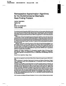
In many applications, there will also exist a more e�cient randomized variant of our algorithm. When analyzing one of these algorithms, we shall estimate only the expected running time. The primary reason for this is that since the running time of any randomized algorithm exceeds twice its expectation with probability at most 1/2, if we make k independent trials of the algorithm, allowing twice the expectation for each trial, then the probability that none of these trials completes the computation is at most 2?k . Thus, by increasing the running time by a logarithmic factor, we can always convert the statement about expectation to one that holds with high probability. In fact, for some of our applications, the stronger statement can be made with no degradation in the bound. Furthermore, the improved e�ciency of these randomized algorithms can be obtained while maintaining the same worst-case running time as the deterministic version. All of the problems in our framework are known to be solvable in polynomial time (without relaxing the right-hand-sides). Consider the problem of packing the vertices of a polytope P subject to the constraints Ax � b. We can apply the ellipsoid method to solve the dual problem, which has a constraint for every vertex of P , since the separation subroutine for the dual problem can be solved with the optimization subroutine for P . The problem can be solved more e�ciently by the algorithm of Vaidya [28]; it obtains the optimal value in O(mL) calls to an optimization subroutine for P plus O(mM(m)L) additional time; L and M(m) denote the binary size of the problem and the time needed to invert m by m matrices, respectively. Alternatively, one can apply the other linear programming algorithm of Vaidya [29] for problems where the polytope P can be described with few variables. Furthermore, if the problem has an appropriate network structure then the ideas of Kapoor and Vaidya [13] can be used to speed up the matrix inversions involved. The algorithm in [28] obtains an optimal dual solution to a fractional packing or covering problem, but no primal solution. By a perturbation agument we can assume that the optimal dual solution is unique, and a primal solution can be obtained by solving a linear problam with T variables and m inequalities, if Vaidya's algorithm uses T calls to the separation subroutine for the dual linear program. We can use Vaidya's algorithm [29] to solve this linear program. The parameter L in the bound of either linear programming algorithm of Vaidya depends on the quality of the starting solution; for example, in [29], it depends on how close the point is to the central path. In some applications, such as the bipartite matching problem, it is possible to nd a starting solution with L = log(n�?1 ), which is, roughly speaking, the number of bits of accuracy required [9]. Unfortunately, we do not know of comparable results for any of our applications. For two of our applications, the bin-packing problem and the Held-Karp bound, such results would yield algorithms with running times that clearly improve on the algorithms based on the approach presented here. Our algorithm outperforms Vaidya's algorithm if � is large (e.g., a constant), � is small, or the optimization subroutine for P is faster than matrix inversion. In many cases, � is not su�ciently small (even exponential), so in Section 4 we give techniques that often reduce �. Figure 1 summarizes the comparison of our algorithm to Vaidya's for our applications, giving the speedup over his algorithms [28, 29] when we assume that � > 0 is any constant, and ignore polylogarithmic factors. A function f (n) is said to be � (g (n)) if there exists a constant c such 3
Application Preemptive scheduling of N jobs on M machines Nonpreemptive scheduling of N jobs on M machines Held-Karp bound on N -city TSP with triangle inequality Min-cost K -commodity ow in M -edge N -node graph Cutting-stock with M widths of nals Job shop scheduling of N �-operation jobs on M machines Embedding an N -node bounded degree graph into a bounded degree graph with ux �.
Deterministic Time O� (MN 2 )
� (M 2:5 N 1:5 )
Speedup
Randomized Time O� (MN )
� (N 2:5 M 2:5 )
O� (M 2 N )
�(N )
O� (MN )
� (MN )
O� (N 5 )
{
O� (N 4 )
�( (N )N ?2 )
O� (K 2M 2 )
� (M :5 NK 1:5 )
O� (KM 2 )
� (M :5 NK 2:5 )
O� (M 2 )
� (M 2 (M ))
O� (M 2 )
� (M (M ))
O� ((N�M )2 + (N�)3 )
� (N 6:5 �4 )
|
|
O� (N 3 �1 )
� (N 2 )
O� (N 2 �1 )
� (N 3 )
M
Speedup
M
M
Figure 1: Summary of the performance of the described algorithms that f (n) logc n � (g (n)); we de ne O� analogously. Our approach extends a method previously applied to nd approximate solutions to multicommodity ow problems, rst by Shahrokhi & Matula [26], and later by Klein, Plotkin, Stein & Tardos [17] and Leighton, Makedon, Plotkin, Stein, Tardos & Tragoudas [20]. Recently, extensions of this method to other applications were found independently by Grigoriadis & Khachiyan [10]. An important theoretical aspect of our results is their connection to Lagrangean relaxation. The main idea of our algorithm is as follows. We maintain a point x 2 P that does not satisfy Ax � b, and repeatedly solve an optimization problem over P to nd a direction in which the violation of the inequalities can be decreased. To do this, we de ne a \penalty" y on the rows of Ax � b. Rows with ai x large relative to bi get a large penalty, other rows get smaller penalties. We relax the Ax � b constraints, and instead solve the Lagrangean relaxed problem min(yAx~ : x~ 2 P ). The idea is that a large penalty tends to imply that the resulting point x~ improves the corresponding inequality. We then set x := (1 ? � )x + � x~, where � is a suitably small number, and repeat. These ideas are often used to obtain empirically good algorithms for solving linear programs; however, unlike previous methods, we give a rule for adjusting the penalties for which a theoretical analysis proves a very favorable performance in many applications. Lagrangean relaxation has been recognized as an important tool for combinatorial optimization problems since the work of Held & Karp on the traveling salesman problem [12]; in our discussion of this application (in Section 5) we examine the relationship between our algorithm and the traditional approach. As in [17], our algorithms can also be modi ed to generate integral approximate solutions and thus yield theorems relating the linear and fractional optima along the lines of Raghavan & Thompson [25] and give alternative deterministic algorithms to obtain the results of Raghavan [24]. The modi ed algorithm is, in some cases, more e�cient than the original algorithm, due 4
to the fact that it terminates as soon as it can no longer improve the current solution while maintaining integrality. We will discuss this integer version of the packing algorithm at the end of Section 2, and use the algorithm for the job-shop and network embedding problems in Section 5. For simplicity of presentation, throughout the paper we shall use a model of computation that allows the use of exact arithmetic on real numbers and provides exponentiation as a single step. In [20], it has been shown that the special case of the algorithm for the multicommodity
ow problem can be implemented in the RAM model without increasing the running time. Analogously, we can use approximate exponentiation and a version of the algorithm that relies only on a subroutine to nd a nearly optimal solution over the polytope P , and hence avoid the need for exponentiation as a step. However, in order to convert the results to the RAM model, we need to perform further rounding; we must also limit the size of the numbers throughout the computation. It is easy to limit the numbers by a polynomial in the input length, similar to the size of the numbers used in exact linear programming algorithms. However, we do not know how to nd an �-approximate solution using polylogarithmic precision for the general case of the problems considered.
2 The Fractional Packing Problem The fractional packing problem is de ned as follows:
9?x 2 P such that Ax � b, where A is an m � n matrix, b > 0, and P is a convex set in Rn such that Ax � 0 for each x 2 P .
Packing:
We shall use ai to denote the ith row of A and bi to denote the ith coordinate of b. We shall assume that we have a fast subroutine to solve the following optimization problem for the given convex set P and matrix A: Given an m-dimensional vector y � 0, nd x~ 2 P such that:
cx~ = min(cx : x 2 P ); where c = y tA:
(1)
For a given error parameter � > 0, a vector x 2 P such that Ax � (1+ �)b is an �-approximate solution to the Packing problem. In contrast, a vector x 2 P such that Ax � b is called an exact solution. An �-relaxed decision procedure either nds an �-approximate solution or correctly concludes that no exact solution exists. The running time of our relaxed decision procedure depends on the width of P relative to
5
Ax � b, which is de ned by ai x : � = max max i x2P b
(2)
i
In general, � might be large, even superpolynomial in the size of the problem. We shall discuss techniques to reduce the width in Section 4.
Relaxed Optimality. Consider the following optimization version of the Packing problem: min(� : Ax � �b and x 2 P );
(3)
and let �� denote its optimal value. For each x 2 P , there is a corresponding minimum value � such that Ax � �b. We shall use the notation (x; �) to denote that � is the minimum value corresponding to x. A solution (x; �) is �-optimal if x 2 P and � � (1 + �)�� . If (x; �) is an �-optimal solution with � > 1 + �, then we can conclude that no exact solution to the Packing problem exists. On the other hand, if (x; �) is a solution with � � 1 + �, then x is an �-approximate solution to the Packing problem. Linear programming duality gives a characterization of the optimal solution for the optimization version. Let y � 0, y 2 Rm denote a dual solution, and let CP (y ) denote the minimum cost cx for any x 2 P where c = y tA. The following inequalities hold for any feasible solution (x; �) and dual solution y : �ytb � y tAx � CP (y): (4) Observe that both y tb and CP (y ) are independent of x and �. Hence, for any dual solution y, �� � CP (y)=y tb. The goal of our algorithm is to nd either an �-approximate solution x, or an �-optimal solution (x; �) such that � > 1 + �. In the latter case we can conclude that no exact solution to the Packing problem exists. The �-optimality of a solution (x; �) will be implied by a dual solution y such that (1 + �)CP (y )=y tb � �. Since � > 1 + �, it follows that CP (y)=y tb > 1; hence, �� > 1 and no exact solution to the Packing problem exists. Linear programming duality implies that there exists a dual solution y � for which CP (y � )=y �tb = �� . Hence, for optimal (x�; ��) and y � , all three terms in (4) are equal. Consider an error parameter � > 0, a point x 2 P satisfying Ax � �b, and a dual solution y. We de ne the following relaxed optimality conditions: (P 1) (1 ? �)�y tb � y t Ax; (P 2) y tAx ? CP (y ) � �(y t Ax + �y tb).
Lemma 2.1 If (x; �) and y are feasible primal and dual solutions that satisfy the relaxed optimality conditions P 1 and P 2 and � � 1=6, then (x; �) is 6�-optimal. 6
Proof : From P 1 and P 2 we have that CP (y) � (1 ? �)y tAx ? ��y tb � (1 ? �)2�y tb ? ��y tb � (1 ? 3�)�y tb: Hence, � � (1 ? 3�)?1CP (y )=(y tb) � (1 ? 3�)?1�� � (1 + 6�)�� .
The Algorithm. The core of the algorithm is the procedure Improve-Packing, which takes as input a point x 2 P and an error parameter � � 0. Given x, it computes �0 , the minimum � such that Ax � �b is currently satis ed. Improve-Packing produces a new feasible solution (x; �) such that x is 6�-optimal or � � �0 =2. It uses a dual solution y de ned as a function of
x, where yi = b1 e�a x=b ; we call this choice of y the dual solution corresponding to x. We will choose � so that the relaxed optimality condition P 1 is satis ed for (x; �) and its corresponding dual solution. Thus, if the current solutions (x; �) and y satisfy P 2, then � is su�ciently close to optimal, and Improve-Packing terminates. Otherwise, we nd a point x~ 2 P that attains the minimum CP (y ), and modify x by setting x (1 ? � )x + � x~. Although a single update of x might increase its corresponding �, we will show that a sequence of such updates gradually reduces �. i
i
i
Lemma 2.2 If � � 2�?1�?1 ln(2m�?1), then any feasible solution (x; �) and its corresponding dual solution y satisfy P 1. Proof : For this proof, it is useful to introduce a localized version of P 1:
(P^ 1) For each i = 1; : : :; m; (1 ? �=2)�bi � ai x or yi bi � 2m� y t b. Let I = fi : (1 ? �=2)�bi � ai xg. Condition P^ 1 implies P 1, since X X X X �ytb = � yi bi + � yi bi � 1 ?1�=2 yi ai x + � 2�m y tb � 1 ?1�=2 ytAx + 2� �y tb; i2I i62I i2I i62I and therefore (1 ? �)�y tb � (1 ? �=2)2 �y tb � y tAx.
Next wePhave to show that the hypothesis of the lemma implies that P^ 1 is satis ed. Notice that y tb = i e�a x=b . By the minimality property of � we have that y t b � e�� . Consider any row i for which ai x < (1 ? �=2)�bi. This implies that yi bi < e(1?�=2)��, and so yi bi=(y tb) < e?���=2 � �=(2m). Hence, P^ 1 is satis ed. i
i
At the beginning of Improve-Packing (see Figure 2), � is set to 4�?0 1�?1 ln(2m�?1); hence, the relaxed optimality condition P 1 is satis ed throughout the execution of the procedure. The following lemma shows that moving the right amount towards a minimum-cost point x~ results P in a signi cant decrease in the potential function � = y tb = i e�a x=b . i
i
Lemma 2.3 Consider a point x 2 P and an error parameter 0 < � � 1 such that x and its corresponding dual solution y have potential function value � and do not satisfy P 2. Let x~ 2 P 7
Improve-Packing(x; �)
� . maxi aix=bi ; � 4�?0 1 �?1 ln(2m�?1); � 4�� While maxi aix=bi � �0=2 and x and y do not satisfy P 2 For each i = 1; : : :; m: set yi b1 e�a x=b : Find a min-cost point x~ 2 P for costs c = yt A. Update x (1 ? �)x + �~x. Return x.
�0
i
i
i
Figure 2: Procedure Improve-Packing. � . De ne a new solution by x^ = (1 ? � )x + � x~, attain the minimum CP (y ). Assume that � � 4�� and let �^ denote the potential function value for x^ and its corresponding dual solution y^. Then � ? �^ � �����.
Proof : By the de nition of �, Ax � �b and Ax~ � �b. This implies that �� jai x ? ai x~j=bi � �=4 � 1=4. Using the second-order Taylor theorem, we see that if j�j � �=4 � 1=4 then, for all x, ex+� � ex + �ex + 2� j�jex. Setting � = ��(ai x~ ? aix)=bi, we see that y^i � yi + b1 ��(ai x~b ? aix) e�a x=b + b1 ��� jai2x~b ? aixj e�a x=b i i i i 1 1 � yi + �� b (aix~ ? aix)yi + ��� 2b (aix~ + aix)yi: i
i
i
i
i
i
Using this inequality to bound the change in the potential function, we get X X X � ? �^ = (yi ? y^i )bi � �� (aix ? ai x~)yi ? �� 2� (ai x + ai x~)yi i i i � = �� (y tAx ? y t Ax~) ? �� 2 (y t Ax + y t Ax~) � �� (y tAx ? CP (y )) ? ���y t Ax:
The fact that P 2 is not satis ed implies that the decrease in � is at least �����.
� , which implies that the decrease in the During Improve-Packing, � is set equal to 4�� potential function due to a single iteration is ( �2�� �). Observe that throughout the execution of Improve-Packing we have e��0=?2 1� � � me��0 . If the input solution is O(�)-optimal, then we have the tighter bound, e�(1+O(�)) �0 � � � me��0 . Together with the previous lemma, this can be used to bound the number of iterations in a single call to Improve-Packing.
Theorem 2.4 The procedure Improve-Packing terminates after O(�?3�?0 1� log( m�?1)) iter?1
ations. If �0 is O(�)-optimal, then Improve-Packing terminates after O(�?2 �0 � log(m�?1 )) iterations. We shall use the procedure Improve-Packing repeatedly to nd an �0 -approximate solution for any given �0 > 0. We rst nd a 1-approximate solution, thereby solving the problem for 8
�0 � 1, and then show how to use this solution to obtain an �0 -approximate solution for any smaller value of �0 . Set � = 1=6, and call Improve-Packing with an arbitrarily chosen solution x 2 P ; repeatedly call this subroutine with the output of the previous call until the resulting solution (x; �) is 6�-optimal or � � 1 + 6�. If, at termination, � � 1 + 6� = 2, then x is a 1-approximate solution. Otherwise, � > 2 and x is 1-optimal, and hence no exact solution exists. The rst part of Theorem 2.4 implies that the number of iterations during such a call to Improve-Packing with input (x; �) is O(�?1� log m). Since this bound is proportional to �?1 and it at least doubles with every call, the number of iterations during the last call dominates the total in all of the calls, and hence O(� log m) iterations su�ce overall.
If �0 < 1, then we continue with the following �-scaling technique. The rest of the computation is divided into scaling phases. In each phase, we set � �=2, and call Improve-Packing once, using the previous output as the input. Before continuing to the next phase, the algorithm checks if the current output (x; �) satis es certain termination conditions. If x is an �0 -approximate solution, then the algorithm outputs x and stops; otherwise, if � > 1 + 6�, the algorithm claims that no exact solution exists, and stops. First observe that if the algorithm starts a new phase, the previous output (x; �) has � � 1 + 6� � 2, and this is the new input. As a result, for each �-scaling phase, the output is an exact solution or is 6�-optimal. Hence, if the output of a phase (x; �) has � > 1, then x is 6�-optimal; if � > 1 + 6�, then the algorithm has proven that no exact solution exists. Furthermore, if no such proof is found by the point when � � �0 =6, the output (x; �) has � � 1 + 6� � 1 + �0 ; x is an �0 -approximate solution. Finally, note that for each phase, the input is a 12�-optimal solution with respect to the new value of �. The second part of Theorem 2.4 implies that the number of iterations needed to convert this solution into a 6�-optimal one is bounded by O(�?2� log(m�?1 )). Since the number of iterations during each scaling phase is proportional to the current value of �?2 and this value doubles each phase, the bound for the last scaling phase dominates the total for all scaling phases. An iteration of Improve-Packing consists of computing the dual vector y and nding the point x~ 2 P that minimizes the cost cx, where c = y tA. Assuming that exponentiation is a single step, the time required to compute y is O(m) plus the time needed to compute (or maintain) Ax for the current point x.
Theorem 2.5 For 0 < � � 1, repeated calls to Improve-Packing can be used so that the
algorithm either nds an �-approximate solution for the fractional packing problem or else proves that no exact solution exists; the algorithm uses O(�?2� log(m�?1 )) calls to the subroutine (1) for P and A, plus the time to compute Ax for the current iterate x between consecutive calls. Notice that the running time does not depend explicitly on n, the dimension of P . This makes it possible to apply the algorithm to problems de ned with an exponential number of variables, assuming we have a polynomial-time subroutine to compute a point x 2 P of cost CP (y) given any positive y, and that we can compute Ax for the current iterate x in polynomial time. As we have mentioned in the introduction, Theorem 2.5 is an extension of a method previously applied to nd approximate solutions to multicommodity ow problems, rst by Shahrokhi & Matula [26], and later by Klein, Plotkin, Stein & Tardos [17] and Leighton, Makedon, Plotkin, 9
Stein, Tardos & Tragoudas [20]. Recently, extensions of this method were also found independently by Grigoriadis & Khachiyan [10]. The algorithm of Grigoriadis & Khachiyan is better in that the number of iterations is a factor of log(m�?1)= log m less than claimed in Theorem 2.5.
Randomized Version. In some cases, the bound in Theorem 2.5 can be improved using randomization. This approach was introduced by Klein, Plotkin, Stein, & Tardos [17] in the context of multicommodity ow; we shall present other applications in Section 5. Let us assume that the polytope P can be written as a product of polytopes of smaller dimension, i.e., P = P 1 � � � � � P k , where the coordinates of each vector x can be partitioned into (x1; : : :; xk) and x 2 P if and only if x` 2 P `, ` = 1; : : :; k. The inequalities Ax � b can P ` ` then be written as A x � b. We assume that for each x 2 P , 0 � A` x` � �`b, ` = 1; : : :; k. P ` ` Clearly, � � ` � . A subroutine to compute CP (y ) for P consists of k subroutines, where the `th subroutine minimizes cx` subject to x` 2 P ` for costsPof the form c = y t A`. Randomization speeds up the algorithm by roughly a factor of k if � = ` �` and either �` = �^ for each `, or the k subroutines have the same time bound. This assumption is satis ed, for example, in the multicommodity ow problem considered in [20]. One way to de ne the multicommodity ow problem as a packing problem is to let P ` be the polytope of all feasible ows satisfying the `th demand and the capacity constraints x` � u, and let the matrix Ax � b describe the joint capacity constraints P` x` � u. For this problem we get that �` = 1 for every `. We shall present other applications in Section 5. The idea of the more e�cient algorithm is as follows. To nd a minimum-cost point x~ in P , Improve-Packing calculates k minimum-cost points x~` 2 P `, ` = 1; : : :; k. Instead, we will choose ` at random with a probability that depends on �` (as described below), compute a single minimum-cost point x~` , and consider perturbing the current solution using this x~` . The perturbation is done only if it leads to a decrease in �. In order to check if P 2 is satis ed by the current solution, it would be necessary to compute CP (y ). This is no longer done each iteration; instead, this condition is checked with probability 1=k. This particular method of randomizing is an extension of an idea that Goldberg [7] has used for the multicommodity ow problem, and was also independently discovered by Grigoriadis & Khachiyan [10]. The key to the randomized version of our algorithm is the following lemma. The proof of this lemma is analogous to the proof of Lemma 2.3.
Lemma 2.6 Consider a point (x1; : : :; xk) 2 P 1 � � � � � P k , with corresponding dual solution y and potential function value �, and an error parameter �, 0 < � � 1. Let x~s be a point in P s that minimizes the cost cs xs, where cs = y tAs , s = 1; : : :; k, and assume that � s � minf�=(4�s�); 1g. De ne a new point by changing only xs , where xs (1 ? � s )xs + � sx~s . If �^ denotes the potential function value of the new solution, then � ? �^ � �� s ((1 ? �)y t As xs ? y t Asx~s ). In this lemma, we have restricted � s � 1 to ensure that the new point is in P ; to get the maximum improvement, the algorithm uses � s = minf1; �=(4��s)g. Since the algorithm changes x only when the update would decrease the potential function, the decrease in the potential 10
s� where �s = maxf((1 ? �)y tAs xs ? y t Asx~s ); 0g. function associated with updating xs is �� P s s s 0 Let S = fs : 4�� < �g and de ne � = s62S � : The probability (s) with which we pick an index s is de ned as follows:
(s) =
(
�s
2�0 1 2jS j
for s 62 S for s 2 S
Using Lemma 2.6, we get the following theorem:
Theorem 2.7 For 0 < � � 1, repeated calls to the randomized version of Improve-Packing
can be used so that the algorithm either nds an �-approximate solution for the fractional packing P ` ` A x � b, or else proves that problem de ned by a polytope P = P 1 � � � �� P k and inequalities P ` ? 2 ` no exact solution exists; the algorithm is expected to take O(� ( ` � ) log(m�?1 ) + k log(��?1)) iterations, each of which makes one call to the subroutine (1) for P ` and A` , for a single value P ` ` of ` 2 f1; : : :; kg, plus the time to compute ` A x for the current iterate (x1; : : :; xk) between consecutive calls. Proof : We rst analyze a single call to the randomized variant of Improve-Packing, and show P ` ?1 ? 3 that it is expected to terminate within O(� ( ` � )�0 log(m�?1 ) + �?1 k) iterations. There are two types of iterations: those where P 2 is satis ed, and those where it isn't. We bound these separately. In the former case, since the algorithm checks whether P 2 is satis ed with probability 1=k, and if so, the algorithm terminates, we expect that O(k) of these iterations will su�ce to detect that P 2 is satis ed, and terminate. In the latter case, we will showPthe expected decrease of the potential function � during oneP iteration is at least minf�2�=(8 ` �`); ln(2m�?1)=kg�. Since P 2 is not satis ed, we have that s �s � ���, where �� s�s is the decrease in � associated with updating xs. Using this fact and applying Lemma 2.6, we see that the expected decrease in � is X
s
�� s�s (s) =
X
s62S
s X � 4��s� � 2��0 �s + 2j�S j �s �
s2S
�X k
� � � � � � � min 8 P �` ; 2k �s � min 8 P �` ; 2k ���: ` ` s=1 Since � � 2�?1�?1 ln(2m�?1), the claimed bound on the expected decrease of � follows.
We use a result due to Karp [16] to analyze the number of iterations used by the randomized version of Improve-Packing. Let �� denote the ratio of upper and lower bounds on the potential function � during a single execution of Improve-Packing. Each iteration of the algorithm when P 2 is not satis ed is expected to decrease the potential function to p�, where p = 1 ? minf�2 �=(8 P` �`); ln(2m�?1)=kg; let b = 1=p. The potential function never increases. Let the random variable T denote the number of iterations of the algorithm when P 2 is not satis ed. Karp proved a general result which implies that
Prob(T � logb �� + ! + 1) � p!?1pblog
b
�� c+1 �
�:
11
(5)
P
To bound the expected number of iterations, we estimate j Prob(T � j ); since p < 1, (5) implies that this expectation is O(logb �� ). Note that �� � me��0=2 , and in the case when the see that the randomizedPversion of Improveinput is O(�)-optimal, �� � me���0 . Hence we P ` ? 2 Packing is expected to terminate in O(� ( ` � )� + �?1 k) = O(�?3( ` �` )�?0 1 log(m�?1 ) + �?1 k) iterations, and is an �?1 factor faster if the input is O(�)-optimal. We use this randomized version of Improve-Packing repeatedly to obtain an �0 -approximate solution in exactly the same way as in the deterministic case. First we set � = 1=6, and then we use �-scaling. The total expected number of iterations is the sum of the expectations over all calls to Improve-Packing . The expected number of iterations in each call to P ` ?1 Improve-Packing with P � = 1=6 is O(( ` � )�0 log m + k), and each call during �-scaling is expected to have O(�?2 ( ` �`) log(m�?1 ) + k) iterations. For both of these bounds, the rst term is nearly identical to the bound for the deterministic case. There are at most log � calls to Improve-Packing with � = 1=6, and log �?0 1 calls during �-scaling, and hence there are P ` ? 2 ? 1 O(�0 ( ` � ) log(m�0 ) + k log(��0?1 )) iterations expected in total. To complete the proof, we must also observe that the routine to check P 2 is expected to be called in only an O(1=k) fraction of the iterations. This implies the theorem. In fact, it is straightforward to bound the expected number of calls to optimize over each
P ` , ` = 1; : : :; k, by O(�?2 �` log(m�?1 ) + log(��?1)). Let T ` denote the time required for the minimization over P ` ,P` = 1; : : :; k, and let T denote the time required for the minimization over P . Assume that � = ` �` and T = P` T ` . Notice that if we have, in addition, that T ` = T=k for each ` = 1; : : :; k, or �` = �=k for each ` = 1; : : :; k, then the time required for running the subroutines in the randomized version is expected to be a factor of k less than was required in the deterministic version. P
P
If � = ` �` and T = ` T ` , then we can combine the deterministic and the randomized algorithms in a natural way. If �` = �=k for each `, or the k subroutines have the same time bound, then by running one iteration of the deterministic algorithm after every k iterations of the randomized one, we obtain an algorithm that simultaneously has the expected performance of Theorem 2.7 and the worst-case performance of Theorem 2.5, except that it will need to compute Ax (for the current solution x) k times more often than is required by Theorem 2.5. Finally, in the introduction, we mentioned that results about expectation could be converted into results that hold with high probability by repeatedly running the algorithm for twice as long as its expected running time bound. In fact, the structure of our algorithm makes this \restarting" unnecessary, since the nal solution obtained by Improve-Packing is at least as good as the initial solution. Thus, all of our results can be extended to yield running time bounds that hold with high probability, without changing the algorithm.
Relaxed Versions. It is not hard to show that our relaxed decision procedure for the packing
problem could also use a subroutine that nds a point in P of cost not much more than the minimum, and this gives a bound on the number of iterations of the same order of magnitude as the original version. 12
Theorem 2.8 If the optimization subroutine (1) used in each iteration of Improve-Packing is replaced by an algorithm that nds a point x~ 2 P such that y tAx~ � (1 + �=2)CP (y ) + (�=2)�y tb for any given y � 0, then the resulting procedure yields a relaxed decision procedure for the packing
problem; furthermore, in either the deterministic or the randomized implementations, the number of iterations can be bounded exactly as in Theorems 2.5 and 2.7, respectively. Proof : It is easy to prove that the analog of Lemma 2.3 remains valid, using � � �=(8��). The only change in the proof is to use the second-order Taylor theorem with j� j � �=8 � 1=8, in order to bound the second-order error term for ex+� by �j� jex=4; this yields that the improvement in the potential function is at least (�=2)����. Lemma 2.6 can be modi ed similarly. Since this improvement is of the same order, the rest of the proof follows directly from these lemmas.
In some applications, there is no e�cient optimization subroutine known for the particular polytope P , as in the case when this problem is NP-hard. However, Theorem 2.8 shows that it su�ces to have a fully polynomial approximation scheme for the problem. Another use of this approximation is to convert our results to the RAM model of computation. In this paper we have focused on a model that allows exact arithmetic and assumes that exponentiation can be performed in a single step. As was done in [20] for the multicommodity
ow problem, we can use approximate exponentiation to compute an approximate dual solution y~ in O(m log(m��?1)) time per iteration. This dual has the property that if we use c~ = y~tA in the optimization routine, then the order of the number of iterations is the same as in the stronger model. This still does not su�ce to convert the results to the RAM model, since we must also bound the precision needed for the computation. It is easy to limit the length of the numbers by a polynomial in the input length, similar to the length of the numbers used in exact linear programming algorithms. However, it might be possible to nd an �-approximate solution using decreased precision, as was done in [20] for the multicommodity ow problem. We leave this as an open problem. In the application to the minimum-cost multicommodity ow problem, even approximate optimization over P will be too time consuming, and we will use a further relaxed subroutine. In order to be able to use this relaxed subroutine, we must adapt the algorithm to solve a relaxed version of the packing problem itself. The relaxed packing problem is de ned as follows: Relaxed Packing: Given � > 0, an m � n matrix A, b > 0, and convex sets P and P^ such
that P � P^ and Ax � 0 for each x 2 P^ , nd x 2 P^ such that Ax � (1 + �)b, or show that 6 9x 2 P such that Ax � b. The modi ed algorithm uses the following subroutine:
13
Given an m-dimensional vector y � 0, nd x~ 2 P^ such that:
ytAx~ � min(y tAx : x 2 P ):
(6)
It is easy to adapt both the algorithms and the proofs for the relaxed problem using this subroutine. For example, it is necessary to change only the second relaxed optimality condition, which becomes: (P^ 2) y tAx ? y tAx~ � �(y t Ax + �y tb), where (x; �) and y denote the current solution in P^ and its corresponding dual, and x~ denotes the solution returned by subroutine (6). Furthermore, � is determined by �^, the width of P^ with respect to Ax � b. We shall state the resulting theorem for the case when P and P^ are in the product form such that P = P 1 � � � � � P k , P^ = P^ 1 � � � � � P^ k , P ` � P^ ` , and 0 � A` x` � �^` b for ` = 1; : : :; k.
Theorem 2.9 The relaxed packing problem can be solved by a randomized algorithm that is P
expected to use a total of O(�?2 ( ` �^`) log(m�?1 )+ k log(^��?1 )) calls to any of the subroutines (6) for P ` , P^ ` and A` x` � b, ` = 1; : : :; k, or by a deterministic algorithm that uses O(�?2�^ log(m�?1 )) P calls for P ` , P^` and A` x` � b, for each ` = 1; : : :; k, plus the time to compute ` A` x` , ` = 1; : : :; k; for the current iterate (x1 ; : : :; xk ) between consecutive calls.
Integer Packing. In some cases, a modi ed version of the packing algorithm can also be used to nd near-optimal solutions to the related integer packing problem. This approach is a generalization of the approach used in [17] to obtain integer solutions to the uniform multicommodity ow problem. In Section 5, we will apply this algorithm to the job-shop scheduling problem and the network embedding problem. To simplify notation, we outline the modi cation to Improve-Packing to nd integer solutions for the case when P is not in product form. If the input solution xPis given explicitly as a convex combination of points xp 2 P returned by the subroutine, x = p � p xp , then each iterate produced by the algorithm is maintained as such a convex combination. Furthermore, if the values � p for the input are all integer multiples of the value of � for this call to the algorithm, then this property will also be maintained throughout its execution. The original version of the packing algorithm updates x by setting it equal to (1 ? � )x + � x~, where x~ 2 P is the point returned by the subroutine. Even if both x and � x~ are integral the new point (1 ? � )x + � x~ might not be. The modi ed algorithm computes y t Axp for every point xp in the convex combination. It selects the point xq with maximum y t Axq , and updates x to x + �(~x ? xq ). Since the current iterate is represented as a convex combination where each � p is an integer multiple of � , the updated point is in P ; furthermore, the updated point can be similarly represented. To bound the number of iterations, we again use the potential function 14
�, and the same calculation as in Lemma 2.3 shows that the decrease in � during one iteration is at least �� (1 ? �)y t Axq ? CP (y ). Since y tAxq � y t Ax by the choice of q , it follows that this decrease is at least �����; thus we get an identical bound for the number of iterations for this modi ed version of the algorithm. The disadvantage of this version is that we need more time per iteration. In addition to the call to the subroutine, we must nd the current solution xq with maximum y tAxq . We state the resulting theorem for the version of Improve-Packing for packing problems P ` ` 1 k in the product form P = P � � � � � P and inequalities ` A x � b, where 0 � A` x` � �` b for each x` 2 P ` , ` = 1; : : :; k. The algorithm maintains each x` 2 P ` as a convex combination of points in P ` returned by the subroutine with coe�cients that are integer multiples of the current value � ` . We further modify the deterministic version in order to maintain � as large as possible: in each iteration, we will update only one x` , deterministically choosing ` to maximize �� `�` ; the analysis of the randomized algorithm is based on the fact that the expected decrease of � is the expectation of �� ` �` , and so by choosing the maximum, we guarantee as least as good an improvement in �. Furthermore, in contrast to the randomized version, we still check if P 2 holds each iteration, and so there is no need to count iterations when P 2 is satis ed, but this is not detected.
Theorem 2.10 For any �, 0 < � � 1, given an input solution (x1; : : :; xk) 2 P 1 � � � �� P k , where
each x` is represented as a convex combination of solutions returned by the subroutine (1) for P ` and A`, and the coe�cients are integer multiples of the current step size � `, ` = 1; : : :; k, the modi ed version of Improve-Packing nds a similarly represented solution to the Packing problem which is 6�-optimal, or else the corresponding value of � has been reducedPby a factor of 2. The randomized version of the algorithm is expected to use a total of O(�?0 1�?3 ( ` �`) log(m�?1 ) + k�?1 ) calls to any of the subroutines (1) for P ` and A` , ` = 1; : : :; k; the deterministic version of the algorithm P uses O(�?0 1�?3 ( ` �`) log(m�?1 ) + k�?1 ) calls to the subroutine (1) for P ` and A` , for each ` = 1; : : :; k. If the initial solution is O(�)-optimal, then the number of calls for both the deterministic and randomized versions is a factor of �?1 smaller. We use this result to obtain an integer packing theorem. For simplicity of notation, we shall state the result in terms of �� = max` �` , instead of the individual �` values. We shall assume that there is a parameter d such that each coordinate of any point returned by each subroutine is an integer multiple of d. If each � ` is an integer multiple of 1=d, then the current solution is integral. We will set � ` equal to the minimum of 1 and the maximum value 2r =d that is at most 4��� , where r is an integer. The algorithm will work by repeatedly calling the modi ed version of Improve-Packing, and will terminate as soon as 4�� �� < d1 . The main outline of the algorithm is the same as above. First set � = 1=6, and repeatedly call the modi ed version of Improve-Packing until a 6�-optimal solution has been found. Then we begin the �-scaling phase, and continue until � s becomes too small, where s is such that �s = ��. Unlike the previous algorithms, this algorithm continues even if it has been shown that there does not exist x 2 P such that Ax � b. This algorithm nds an integer point in P , but it might only satisfy a greatly relaxed version of the packing constraints. The following theorem gives a bound on the quality of the solution delivered by this algorithm. The theorem is an extension of a result in [17] for the multicommodity ow problem with uniform capacities. The existence of an integer solution `
15
under similar assumptions has been proven by Raghavan [24]. However, Raghavan constructs the integer solution using linear programming.
Theorem 2.11 Let �0 = max( �� ; (��=d) log m). There exists an integral solution to P` A` x` � �b p with x` 2 P ` and � � �� +O( �0 (��=d) log(mkd)). Repeated calls to the randomized integer version of Improve-Packing nd such a solution (�x; ��) with an expected total of O(kd + k�� log(m)=�� + k log(kd)) calls to any of the subroutines (1) for P ` and A`, ` = 1; : : :; k. A deterministic version of the algorithm uses O(kd + k�� log(m)=�� + k log(kd)) calls to each of the k subroutines.
Proof : We rst analyze the number of iterations of the deterministic algorithm given above, using Theorem 2.10 in a way similar to the analysis of the algorithm for the fractional packing problem. Let (�x; �� ) denote the solution output by the algorithm. First we compute the number of iterations when � = 1=6. The rst term of the bound in Theorem 2.10 depends on �?1, which doubles with each call to Improve-Packing, and so its total contribution can be bounded by its value for the nal call with � = 1=6. Since the value of � changes by at most a factor of 2 during �-scaling, this term contributes a total of O(k�� log(m)=��) iterations to the overall bound. The contribution of the second term is k times the number of times that Improve-Packing is called with � = 1=6; this yields a term of O(k log(�=��)) in the overall bound. To bound the number of iterations during �-scaling, we rst bound the value of � at termination. Focus on the call to Improve-Packing for which � s < 1=d, where s is such that �s = ��. Recall that ��p� � � 2�� throughout �-scaling. Since � s = �(�2 �=(�� log(m�?1))), it su�ces to have � = �( �� log(mkd)=(��d)), in order that � s < 1=d. The total contribution of the rst term of the bound in Theorem 2.10 throughout �-scaling can again be bounded by its value for the nal call to Improve-Packing, which is O(kd). The total contribution of the second term can be bounded by O(k log �?1 ) = O(k log(��d=��)). This yields the claimed bound. The analysis of the randomized version is identical.
Next consider the quality of the solution found. The algorithm can terminate due to reducing
�s below 1=d either while � = 1=6, or during the �-scaling. Suppose that the former option occurs. We know that � s � �=(8��s) = (��=(�� log m)). This implies that �� = O((��=d) log m), and this is within the claimed bound. Next assume that � < 1=6 when � s becomes less than 1=d. Since �� � �� � 2�� and �ps = �(�=(��s)), we see that � s = p �(�2 ��=(�� log(m�?1 ))) in this case. This implies that � = �( �� log(m�?1 )=(d��)), which is O( �� log(mkd)=(d��)). The output, which was obtained at the end of the previous scaling phase, is O(�)-optimal. Therefore, �� meets the claimed bound.
General Problem. Consider the class of problems in the following form: 9?x 2 P such that Ax � b, where A is an m � n matrix, b is an arbitrary vector, and P is a convex set in Rn .
General:
We shall assume that we are given a fast subroutine to solve the following optimization problem for P and A: 16
Given an m-dimensional vector y � 0, nd a point x~ 2 P such that:
cx~ = min(cx : x 2 P ) where c = y tA:
(7)
Given an error parameter � > 0 and a positive tolerance vector d, we shall say that a point x 2 P is an �-approximate solution if Ax � b + �d; an exact solution is a point x 2 P such that Ax � b . The running time of the relaxed decision procedure for this problem depends on the width � of P relative to Ax � b and d, which is de ned in this case by jaix ? bij + 1: � = max max i x2P di
Note that we have added 1 to ensure that the de nition of width for the General problem is consistent with the de nition of width for the Packing problem. We shall show that the General problem can be reduced to the Packing problem. Let the convex set P , the inequalities Ax � b, and the tolerance vector d de ne a General problem with width �. The corresponding Packing problem is de ned as follows. The convex set is P~ = f(x; s) : x 2 P and s = 1g in Rn+1 . The inequalities are de ned as Ax +(�d ? b)s � ~b = �d. Notice that jAx ? bj � (� ? 1)d implies that this convex set and inequalities de ne a Packing problem. The width of the resulting instance of the Packing problem is less than 2. There is a one-to-one correspondence between exact solutions to this Packing problem instance and exact solutions of the General problem instance, and an �~-approximate solution to the Packing problem instance is an �-approximate solution of the General problem instance if we de ne �~ = �=�. Notice that the subroutine (1) required for the packing algorithm is subroutine (7). Theorem 2.5 now implies the following theorem.
Theorem 2.12 For any �, 0 < � < 1, if the General problem has an exact solution, then an �-approximate solution can be found in O(�2�?2 log(m��?1 )) calls to the subroutine (7) for P and A, plus the time to compute Ax for the current iterate x between consecutive calls. Remark In an earlier version of this paper [23] we developed an algorithm analogous to
Improve-Packing for the General problem, instead of the above reduction. We would like to thank an anonymous referee for pointing out this reduction. However, the direct algorithm has the advantage that analogous to Theorem 2.7 we could use randomization to speed up the algorithm for the General problem if the polytope is in product form. The same speedup does not seem to follow from the reduction. Due to the lack of applications we do not include the direct algorithm.
3 The Fractional Covering Problem The fractional covering problem is de ned as follows: 17
Covering: 9?x 2 P such that Ax � b, where A is an m � n matrix, b > 0, and P is a convex set in Rn such that Ax � 0 for each x 2 P .
In this section, we shall describe a relaxed decision procedure for the fractional covering problem whose running time depends on the width � of P relative to Ax � b; as in the previous section, the width is de ned to be maxi maxx2P ai x=bi. We shall assume that we are given a fast subroutine to solve the following optimization problem for P and A: Given an m-dimensional vector y � 0, nd x~ 2 P such that
cx~ = max(cx : x 2 P ); where c = y tA:
(8)
For a given error parameter � > 0, an �-approximate solution to the Covering problem is a vector x 2 P such that Ax � (1 ? �)b; an exact solution is a vector x 2 P such that Ax � b. The Covering problem is a special case of the General problem, and therefore we can use Theorem 2.12 to get a relaxed decision procedure for the problem. In this section we give a more e�cient relaxed decision procedure that is designed directly for the Covering problem. Consider rst the algorithm of Theorem 2.5 when applied to the Covering problem. To reduce the Covering problem to a Packing problem we use �~ = �=�; the width of the resulting Packing problem is only (� + 1)=� due to the assumption that Ax � 0 for each x 2 P . Theorem 2.5 now implies the following: if � = O(�), and the Covering problem has an exact solution, then an �-approximate solution can be found in O(�2�?2 log(m��?1)) calls to the subroutine (8). This running time is proportional to �2. The direct algorithm discussed in this section has the advantage that its running time is linear in �, and it leads to a natural randomized speedup if the problem is in the product form. In the applications discussed in Section 5 the width of the covering problems is large, and therefore this is an important improvement.
Relaxed Optimality. Consider the following optimization version of the Covering problem: max(� : Ax � �b and x 2 P ):
(9)
Let �� denote the optimal value. For each x 2 P there is a corresponding maximum value � such that Ax � �b. We shall use the notation (x; �) to denote that � is the maximum value corresponding to x. A solution (x; �) is �-optimal if x 2 P and � � (1 ? �)�� . The method to solve this problem is analogous to the one used for the fractional packing problem. Let y � 0, y 2 Rm denote a dual solution, and let CC (y ) denote the maximum value of cx for any x 2 P where c = y tA. Let (x; �) denote a feasible solution, and consider the following 18
chain of inequalities: �ytb � y tAx � CC (y): (10) Observe that for any dual solution y , the value CC (y )=y tb is an upper bound on �� . We will use the following two relaxed optimality conditions. (C 1) (1 + �)�y tb � y t Ax (C 2) CC (y ) ? y tAx � �(CC (y ) + y tb): Observe that condition C 2 di�ers from its analog P 2 in that there is an additional factor of � in the last term of P 2. While this change is not important for the correctness of the algorithm, it improves the running time of the algorithm. However, with (C 2) as stated above, we cannot claim that a pair (x; �) and y satisfying condition C 1 and C 2 are �-optimal unless � is close to 1. We have the following lemma instead.
Lemma 3.1 Suppose that (x; �) and y are feasible primal and dual solutions that satisfy the relaxed optimality conditions C 1 and C 2. If � � 1 ? 3�, then there does not exist an exact solution to the fractional covering problem. If � � 1 ? 3�, then x is 3�-optimal. Proof : C 1 and C 2 imply that CC (y) � (1 ? �)?1 (y tAx + �y tb) � (1 ? �)?1((1 + �)� + �)y t b: Consider the case when � � 1 ? 3�. For any dual solution y , �� � CC (y )=(y tb). This implies that � 1 : �� � CC (y) � (1 + �)� + � � 1 + � + � t � �y b �(1 ? �) 1 ? � (1 ? �)(1 ? 3�) 1 ? 3� On the other hand, if � � 1 ? 3�, we have ? 3�) + � < 1: �� � CyCt(by) � (1 + �)(1 1?� Hence, in this case, there is no exact solution to the fractional covering problem.
The Algorithm. The heart of the covering algorithm is the procedure Improve-Cover (see
Figure 3), which is the covering analog of the procedure Improve-Packing. It uses a dual solution y de ned as a function of x, where yi = b1 e?�a x=b for some parameter �; y is the dual solution corresponding to x. Throughout the procedure, the current solution (x; �) and its corresponding dual solution y will satisfy C 1. If C 2 is also satis ed, then we can either conclude that no feasible solution exists, or that � is su�ciently close to optimality, and we can terminate. Otherwise, we nd the point x~ 2 P that attains the maximum CC (y ), and we modify x by moving a small amount towards x~. This will decrease the potential function � = y tb, and gradually increase �. i
i
The following lemma is similar to Lemma 2.2. 19
i
Improve-Cover(x; �)
� . mini aix=bi; � 4�?0 1 �?1 ln(4m�?1); � 4�� While mini aix=bi � 2�0 and x and y do not satisfy C2 For each i = 1; : : :; m: set yi b1 e?�a x=b : Find a maximum-cost point x~ 2 P for costs c = yt A. Update x (1 ? �)x + �~x. Return x.
�0
i
i
i
Figure 3: Procedure Improve-Cover.
Lemma 3.2 If � � 2�?1�?1 ln(4m�?1) and 0 < � < 1, then any feasible solution (x; �) and its corresponding dual solution y satisfy C 1. Proof : For this proof, it is useful to introduce a localized version of C 1.
(C^1) For each i = 1; : : :; m, (1 + �=2)�bi � ai x or ai xyi � 2�m �y tb. Note that C^1 implies that aixyi � (1 + �=2)�yibi + 2�m �ytb:
Summing up over all i, we see that C^1 implies C 1. Next we show that the hypothesis of the lemma implies that C^1 is satis ed. Notice that P ?�a x=b t . By the maximality property of �, we have that y t b is at least e?��. Consider y b = ie any row i for which (1 + �=2)�bi < aix and let �i = ai x=bi. This implies that �i > (1 + �=2)�. If �z � 1, then ze?�z is a monotonically nonincreasing function of z . Since, by de nition of �, we have �i� > �� � 1, we get that aixyi = (aix=bi)e?�a x=b = �i e?�� < (1 + �=2)�e?��(1+�=2) = (1 + �=2)�e?���=2 � �� : y tb ytb ytb e?�� 2m i
i
i
i
i
Next we prove that for anPappropriately chosen � , the new solution signi cantly reduces the potential function � = y tb = i e?�a x=b . i
i
Lemma 3.3 Consider a point x 2 P and an error parameter �, 0 < � � 1, such that x and its corresponding dual solution y have potential function value � and do not satisfy C 2. Let x~ 2 P � . De ne a new solution by x^ = (1 ? � )x + � x~, attain the maximum CC (y ). Assume that � � 4��
and let �^ denote the potential function value for x^ and its corresponding dual solution y^. Then � ? �^ � ��� �.
Proof : By the de nition of �, Ax � �b and Ax~ � �b. This implies that �� jai x ? ai x~j=bi � �=4 � 1=4. Using the second-order Taylor theorem we see that if j�j � �=4 � 1=4, then, for all x, ex+� � ex + �ex + 2� j�jex. Setting � = ��(ai x ? ai x~)=bi, we see that
20
y^i � yi + b1 ��(ai xb ? ai x~) e?�a x=b + b1 ��� jai2xb ? ai x~j e?�a x=b i i i i 1 1 � yi + �� b (aix ? aix~)yi + ��� 2b (aix + aix~)yi: i
i
i
i
i
i
Using this inequality to bound the change in the potential function, we get X X X � ? �^ = (yi ? y^i )bi � �� (aix~ ? ai x)yi ? �� 2� (ai x~ + ai x)yi i i i � t t t t = �� (y Ax~ ? y Ax) ? �� 2 (y Ax~ + y Ax)
= �� (CC (y ) ? y tAx) ? �� 2� (CC (y ) + y tAx) � �� (CC (y ) ? y tAx) ? ���CC (y ):
Since C 2 is not satis ed, the decrease in � is at least ����.
Next we show that the chosen value of � is large enough to guarantee that condition C 1 is always satis ed during the execution of Improve-Cover.
Lemma 3.4 If 0 < � < 1, then throughout the execution of Improve-Cover, the current solution (x; �) has � � 3�0=4. Proof : The value of the potential function � does not increase during the execution of ImproveCover. Initially, � � me?��0 , and for any current solution (x; �), � � e?��. Therefore �0 ? � � �1 ln m � ��0=4 � �0=4:
This implies that � � 3�0=4:
Since we set � = 4�?1 �?0 1 log(m�?1 ), Lemma 3.2 implies that C 1 is satis ed throughout the � , the decrease in the potential function execution of Improve-Cover. Since � is set equal to 4�� 2 due to a single iteration is ( �� �). Observe that during a single call to Improve-Cover we solution is 6�-optimal for � � 1=12, then we have the have e?2��0 � � � me?��0 . If the initial tighter bound, e?�(1+12�)�0 � e?�(1?6�)?1�0 � � � me?��0 . This, together with Lemma 3.3, can be used to bound the number of iterations in a single call to Improve-Cover.
Theorem 3.5 The procedure Improve-Cover terminates in O(�?3� log(m�?1)) iterations. If the initial solution is 6�-optimal for � � 1=12, then Improve-Cover terminates in O(�?2� log(m�?1 ))
iterations.
We use the procedure Improve-Cover repeatedly to nd an �0 -approximate solution. Before this, we must specify how to obtain an initial solution of su�cient quality, which is somewhat 21
more involved than for the packing analog (where any initial solution in P su�ces). For each i = 1; : : :; m, we nd xi 2 P that maximizes aix; this takes m calls to the subroutine. If there exists an i such that max(aix : x 2 P ) < bi , then we can conclude that no exact solution for the P Covering problem exists. Otherwise, we take (1=m) i xi as the initial solution, for which the corresponding value of � is at least 1=m.
Lemma 3.6 With m calls to the subroutine (8) for P and A, we can either nd a solution x 2 P satisfying Ax � (1=m)b, or conclude that there does not exist an exact solution to the Covering problem.
The basic approach to using Improve-Cover to obtain an �0 -approximate solution closely parallels the packing algorithm. First set � = 1=6 and start with the point x 2 P given by the previous lemma; this is a solution (x; �) with � � 1=m. Between consecutive calls to ImproveCover, we increase �0 by at least a factor of 2, and so within log m iterations, Improve-Cover must output an exact solution or else nd feasible primal and dual solutions (x; �) and y that satisfy C 1 and C 2. Suppose the latter occurs. If � � 1 ? 3� = 1=2, then the algorithm concludes that no exact solution exists (by Lemma 3.1); otherwise, � > 1=2 and x is 1=2-optimal. If �0 � 1=2 then the algorithm outputs x and stops; otherwise, we proceed to �-scaling. Each scaling phase decreases � by a factor of 2, and then makes a single call to Improve-Cover. The algorithm checks if the resulting solution (x; �) is an �0 -approximate solution, and if so, outputs x and stops. Otherwise, it checks if � � 1 ? 3�, and if so, claims that no exact solution exists and stops. If neither termination criterion is satis ed, the algorithm proceeds to the next phase. The input to each scaling phase has � � 1 ? 3� � 1=2, and so the output is either an exact solution, or else satis es the relaxed optimality conditions. Note that the output must be 3�-optimal in the only case when further phases are needed. Hence, each call to ImproveCover has an input that is a 6�-optimal solution with the new � � 1=12. Furthermore, the algorithm is guaranteed to stop by the point when � � �0 =3. Improve-Cover uses O(� log m) iterations for each of the O(log m) iterations with � = 1=6, and the number of iterations during �-scaling is dominated by the the number of iterations during the nal call to Improve-Cover, which implies the following theorem.
Theorem 3.7 For 0 < � < 1, repeated calls to Improve-Cover can be used so that the algorithm either nds an �-approximate solution for the fractional covering problem, or proves that no exact solution exists; the algorithm uses O(m + � log2 m + �?2 � log(m�?1)) calls to the subroutine (8) for P and A, plus the time to compute Ax for the current iterate x between consecutive calls.
Randomized Version. As was true for the fractional packing problem, we can use random-
ization to speed up the fractional covering algorithm if the polytope is in product form. Suppose P that P = P 1 �� � ��P k and the inequalities, when written to re ect this structure, are A` x` � b. We assume that 0 � A` x` � �` b for each x` 2 P ` , and ` = 1; : : :; k. In this case, a subroutine (8) to compute CC (y ) for P and A consists of a call to each of k subroutines: subroutine (8) for P ` and A`, ` = 1; : : :; k. Instead of calling all k subroutines each iteration, the randomized algorithm will make a call to the subroutine (8) for P s and As for a single value s 2 f1; : : :; kg. 22
The choice of s is made at random, according to a probability distribution that we will describe below, independently of choices made in other iterations. A tentative modi cation of the current iterate (x1; : : :; xk ) is made, where only the coordinate xs is updated. If this change causes the potential function to decrease, then it is really made; otherwise, the current iterate is unchanged by this iteration. Since CC (y ) is not computed each iteration, we cannot check if C 2 is satis ed; instead, in each iteration, with probability 1=k, the algorithm does the additional work needed to check this condition. As in the case of P the Packing problem, randomization speeds up the algorithm by roughly a factor of k if � = ` �`, and either �1 = �2 = � � � = �k , or the k subroutines have the same time bound. The key to the randomized version of our algorithm is the following lemma, which is analogous to Lemma 2.6.
Lemma 3.8 Consider a point (x1; : : :; xk) 2 P 1 � � � � � P k with corresponding dual solution y
and potential function value �, and an error parameter �, 0 < � < 1. Let x~s be a point in P s that maximizes the cost cs xs , where cs = y t As, s = 1; : : :; k; and assume that � s � minf�=(4�s�); 1g. De ne a new point by changing only xs , where xs (1 ? � s )xs + � sx~s . If �^ denotes the potential function value of the new solution, then � ? �^ � �� s ((1 ? �)y t As x~s ? y t Asxs ). Since the algorithm updates x only when � decreases, the change in � associated with updating xs is �� s �s , where �s = maxf((1 ? �)y tAs x~s ? y t As xs); 0g. We have restricted � s � 1 to ensure that the new point is in P ; to get the maximum improvement, the algorithm sets �` = minf1; �=(4��`)g. Let S = fs : 4��s � �g and de ne �0 = Ps62S �s: The probability (s) with which we pick an index s is de ned as follows:
(s) =
(
�s
2�0 1 2jS j
for s 62 S for s 2 S
Using Lemma 3.8 instead of Lemma 3.3, we get the following theorem:
Theorem 3.9 For 0 < � < 1, repeated calls the randomized version of Improve-Cover can be
used so that the algorithm either nds an �-optimal solution for the fractional covering problem de ned by the polytope P = P 1 �� � �� P k and inequalitiesPP` A` x` � b, or else proves thatPno exact solution exists; it is expected to use a total of O(mk + ( ` �`) log2 m + k log �?1 + �?2 ( ` �`) log(Pm�?1 )) calls to any of the subroutines (8) for P ` and A` , ` = 1; : : :; k, plus the time to compute ` A` x` between consecutive calls. Proof : We nd an initial solution using Lemma 3.6. This requires m calls to the subroutine (8) for each P ` and A` , ` = 1; : : :; k. Hence, we can assume that our initial solution (x; �) has � � 1=m.
Next we analyze a single call to the randomized variant of Improve-Cover, in a way completely analogous to the analysis of the randomized version of Improve-Packing. There 23
are two types of iterations: those where C 2 is satis ed, and those where it isn't. We separately bound the expected number of each of these. For the former, since C 2 is checked with probability 1=k in each iteration, there are O(k) of these iterations expected before the algorithm detects that C 2 is satis ed, and terminates. In the latter case, we shall show that the expected decrease of � P during each iteration is fminf�2 =�0; �?1 log(m�?1)=kg�. Since C 2 is not satis ed, s �s � ��, where �� s�s is the decrease in � associated with updating xs . Using this fact and applying Lemma 3.8, we see that the expected decrease in � is X
s
�� s�s (s) =
X
s62S
s X � 4��s� � 2��0 �s + 2j�S j �s �
�X k
s2S
� � � � � � � min 8�0 ; 2k �s � min 0 ; ��: 8� 2k s=1 Since � = (�?1�?1 log(m�?1)), we get the claimed decrease in �.
To analyze the number of iterations, we once again apply the result of Karp [16]. This implies P ` ?3 that the randomized version of Improve-Cover is expected to terminate in O(( ` � )� log(m�?1 )+ k�?1 �0) iterations, and is a factor of �?1 faster if the initial solution is 6�-optimal for � � 1=12. We use this randomized version of Improve-Cover repeatedly to nd an �0 -approximate solution in exactly the same way as in the deterministic case. First we set � = 1=6, and then use �-scaling. The contribution of terms that depend on �0 or �?1 can be bounded by their value for calls in which these parameters are largest. For the remaining terms, we need only observe that there are O(log m) calls to Improve-Cover with � = 1=6, and O(log �?0 1 ) calls during �-scaling. To complete the proof, we note that condition C 2 is expected to be checked in an O(1=k) fraction of the iterations.
Relaxed Version. It is not hard to see that a subroutine that nds a point in P of cost not
much less than the maximum can be used in the algorithm, and gives a bound on the number of iterations of the same order of magnitude.
Theorem 3.10 If the optimization subroutine (8) used in each iteration of Improve-Cover is replaced by an algorithm that nds a point x~ 2 P such that y t Ax~ � (1 ? �=2)CC (y ) ? (�=2)�y tb for any given y � 0, then the resulting procedure yields a relaxed decision procedure for the fractional covering problem; furthermore, in either the deterministic or the randomized implementations, the number of iterations can be bounded exactly as before, in Theorems 3.7 and 3.9, respectively.
Proof : It is easy to prove that the analogs of Lemmas 3.3 and 3.8 remain valid. The rest of the proof follows from these lemmas.
In some of our applications, the optimization over P required by the original version of the algorithm is di�cult or even NP-hard. However, if there is a fast fully polynomial approximation scheme for the problem, then Theorem 3.10 allows us to use the approximation algorithm instead. 24
4 Decreasing the width � The running times of our algorithms are proportional to the width �. In this section we present techniques that transform the original problem into an equivalent one, while reducing the width. Each of the techniques assumes the existence of a particular fast subroutine related to optimization over P ; di�erent subroutines might be available in di�erent applications.
Relaxation of Integer Programming. In some cases, the primary interest in solving a
particular fractional packing problem is to obtain a lower bound on an integer program of the form: minimize cx subject to A0x � b0 and x 2 P , where the constraints constitute an integer packing problem. As a result, we wish to decide if there exists a fractional solution x 2 P that satis es the constraints Ax � b, that consist of A0 x � b0 and cx � b0, for some value b0. Assume that A � 0, c � 0, and x � 0 for each x 2 P . We shall give a technique to reduce the width of the fractional packing problems that arise in this way. The assumptions that A � 0 and P is in the nonnegative orthant imply that any integer solution must satisfy xj = 0 whenever there exists an index i such that aij > bi. Hence, instead of using P , we can tighten the fractional relaxation, and use P� = fx : x 2 P; xj = 0 if j 2 J g, where J = fP j : 9i such that aij > big. The width �� of P� relative to Ax � b is bounded by � = maxx2P j xj . For example, if the variables of the integer program are restricted to be 0 or 1, we get � � n.
Theorem 4.1 For any �, 0 < � � 1, there is an �-relaxed decision procedure to solve a fractional packing problem that is derived from an integer packing problem satisfying A � 0, c � 0, and x � 0 for each x 2 P , in O(�?2 � log(m�?1 )) calls to the subroutine that nds a minimum-cost point in
the restricted polytope P� , plus the time to compute the value of the left-hand side of the packing constraints for the current iterate after each update. If x � 1 for all x 2 P , then � � n. If P is a direct product of convex sets, then so is P� , and hence the same technique can be applied for speeding up the randomized version of the packing algorithm as well.
Restricting P `. The next technique can be applied for some packing problems where P
is a product of convex sets in smaller dimension. The idea is to de ne the same packing problem using a di�erent polytope that has a smaller width. This technique can be applied for multicommodity ow problems (to obtain the formulation used in [20]) and for the preemptive machine scheduling problem, which will be discussed in the next section. Consider a packing problem de ned by the convex set P = P 1 �� � �� P k , and the inequalities ` ` 1 k ` ` ` ` A x � b. It is easy to see that the convex set P^ = P^ � � � � � P^ , where P^ = fx 2 P : ` ` A x � bg, ` = 1; : : :; k, and the same inequalities de ne the same fractional packing problem, and has � � k. It is possible that one of the polytopes, P^` , ` = 1; : : :; k, is empty, and if so, the optimization routine for P^` will detect this, and thereby prove that there does not exist an exact solution to the original problem. P
25
Theorem 4.2 For any �, 0 < � � 1, there is an �-relaxedPdecision procedure to solve a fractional packing problem de ned by P = P 1 � � � � � P k and ` A` x` � b that is expected to use a
total of O(�?2 k log(m�?1 ) + k log k) calls to a subroutine that nds a minimum-cost point in P^ ` , ` = 1; : : :; k, and a deterministic version that uses O(�?2 k2 log(m�?1)) such calls, plus the time to compute the value of the left-hand side of the packing constraints for the current iterate after each update. Recall that the multicommodity ow problem can be de ned with P ` being the dominant of the convex combinations of all paths from the source of commodity ` to its sink. In this case, optimization over P ` is a shortest path computation, but the parameter � de ned by the problem can be arbitrarily high. The above technique imposes capacity constraints on the
ows of individual commodities (since a ow is a convex combinations of paths). The resulting equivalent formulation has �^ � k, but the required subroutine is the more time consuming minimum-cost ow computation.
Decomposition for Packing Problems. Consider the packing problem de ned by a polytope P and inequalities Ax � b. We introduce a decomposition technique that de nes a related
problem with decreased width by replacing P and A by an equivalent problem in the product form. This decomposition can be used in cases where P is a polytope and we are given a subroutine that is more sophisticated than an optimization routine for P ; the details of this routine will be given below. This technique will be used to solve the minimum-cost multicommodity
ow problem in the next section. For simplicity of presentation, we shall initially work with fractional packing problems where the polytope is a simplex. This is, in fact, without loss of generality, since each packing problem is equivalent to a problem in this form. To see this, let v1 ; : : :; vs denote a list of the vertices of P P . EachPpoint x 2 P can be written as a convex combination of the vertices of P : x = j �j vj , where j �j = 1 and �j � 0; j = 1; : : :; s. If we let �j , j = 1; : : :; s, be the variables of the transformed problem, then this yields a problem in which the polytope is a simplex, possibly with exponentially many variables; the packing constraints are now represented as H� � b, where H = (hij ) and hij = aivj . Observe that this change of coordinates does not change the width. In order to apply the packing algorithm to the transformed problem, we need a subroutine that nds j such that the j th coordinate of the vector y t H is minimum. Substituting the de nition of H , this means that we need a subroutine that nds a vertex vj of P that has minimum cost cvj where c = y t A. Now we show how to obtain an equivalent problem for which the width is roughly half of its original value �. In order to facilitate recursion, we will assume that the simplex is de ned by S = f(�1; �2; : : :; �s) : P �j = d; �j � 0; j = 1; : : :; sg for some d. We introduce two copies of each variable �j : �j1 and �j0 . If we let J 1P= fj : 9i such that hij d > 2mbig, then the new polytope is S 1 � S 0 , where S 0 = (1=2)S = f� : j �j = d=2; � � 0g and S 1 = f� 1 : � 1 2 S 0; �j1 = 0 if j 2 J 1 g. The new system of packing inequalities is H� 1 + H� 0 � b. Note that the width of S 0 relative to H� 0 � b is �=2; for any � 1 2 S 1, X
j
hij �j1 �
X
j 62J 1
(2mbi=d)�j1 � (2mbi=d) 26
X
j
�j1 � mbi; i = 1; : : :; m;
and hence the width of S 1 relative to H� 1 � b is at most m. If we apply the same transformation to S 0, after k = dlog �e applications we obtain a fractional packing problem where thePpolytope is a product of k +1 polytopes, S 1 �� � �� S k � S 0 , and a set of inequalities of the form ` H� ` + H� 0 � b, where S 0 = 2?k S , and S ` = f� ` : � ` 2 2?`S; �j` = 0 if j 2 J ` g where J ` = fj : 9i such that hij d > 2`mbi g. Since, for any � ` 2 S `, X
j
X
hij �j` �
j 62J
`
(2` mbi=d)�j` � (2` mbi=d)
X
j
�j` � mbi; i = 1; : : :; m;
the width of S ` relative to H� ` � b is at most m, ` = 1; : : :; k. Furthermore, the following lemma implies that the new problem is equivalent to the original one.
Lemma 4.3 If the fractional packing problem de ned by S P and H� � b has an exact solution, 1 k 0 then so does the problem de ned by S � � � � � S � S and ` H� ` + H� 0 � b. For any � > 0, any �-approximate solution to the latter problem can be used to nd an �-approximate solution to the former.
Proof : We rst note that if (� 1; : : :; � k ; � 0) is an �-approximate solution to the transformed P ` problem, then � = ` � + � 0 is an �-approximate solution to the original problem.
Now assume that we have an exact solution � to the original problem. We will show that this implies the existence of an exact solution of the transformed problem. In fact, although this is not necessary to prove the lemma, we will give an algorithm to construct such a solution, given the solution for the original problem. Initially, set � 0P= � and � ` = 0, ` = 1; : : :; k.PThe algorithm consists of k phases. In phase `, ` = 1; : : :; k, j �j0 decreases by d=2`, and j �j` increases by the same amount. All other variables are unchanged. Hence, the resulting solution (� 1; � 2; : : :; � k ; � 0) is such that � ` 2 2?` S , ` = 1; : : :; k, and � 0 2 2?k S = S 0. We will perform each phase to ensure that, in fact, each � ` 2 S `, ` = 1; : : :; k. P
In phase `, ` = 1; : : :; k, while j �j0 > d=P 2`, nd j 62 J ` with �j0 > 0, and simultaneously ` 0 ` ` 0 g. This maintains that P H� ` + H� 0 � b. increase �j and decrease � by min f � ; d= 2 ? � j j j j ` P ` 2 S ` . We claim If we continue until j �j0 = d=2`, this ensures that the resulting solution � P that we can always continue while j �j0P> d=2`. Assume, for a contradiction, that for the current solution (� 1; : : :; � k; � 0), we have j �j0 > d=2`, and j 2 J ` whenever �j0 > 0. Hence, for each j such that �j0 > 0, we have a row i(j ) that contains a large coe�cient in the j th 0 `mbi(j )=d. Furthermore, d=2` < P � 0 = P P column: h > 2 i ( j ) j i j :i(j )=i �j : Choose i such that j j P P 0 ` s 0 j :i(j )=i �j > d=(2 m), and consider row i of s H� + H� � b. We get that XX
which contradicts
hij �js +
s
j
P
s H�
X
j
hij �j0 �
X
j :i(j )=i
i hij �j0 > 2 mb d `
X
j :i(j )=i
�j0 > bi ;
s + H� 0 � b.
Having obtained this decomposition, we would like to express these polytopes and these constraints in terms of the original coordinates; we also would like to express the optimization 27
subroutine (1) for S ` and H in terms of a di�erent, more intricate, subroutine for P and A. For the former, we can restate the decomposed problem as P 1 � � � �� P k � P 0 subject to the system P P of inequalities ` Ax` + Ax0 � b, where P 0 = 2?k P and P ` = fx` : x` = j �j` vj ; � ` 2 S ` g, ` = 1; : : :; k. In other words, a point in P ` is 2?` times a convex combination of vertices vj of P , each of which satis es Avj � 2` mb. Thus, in these terms, the basic decomposition lemma can be restated in the following way.
Lemma 4.4 If the fractional packing problem de ned by P and Ax �Pb has an exact solution, then so does the transformed problem de ned by P 1 � : : : � P k � P 0 and ` Ax` + Ax0 � b; where k � dlog �e. For any � > 0, any �-approximate solution to the latter problem can be used to nd an
�-approximate solution to the former.
In order to apply the packing algorithms in Theorem 2.5 and Theorem 2.7 to the transformed problem, we need subroutines that, given a dual solution y , nd a point x` 2 P ` that minimizes the cost c`x` , where c` = y tA, ` = 1; : : :; k. There is a vertex of P ` that attains this minimum; the vertices of P ` are those vertices vj of P that satisfy Avj � 2`mb: Hence, it is su�cient to have the following subroutine with � = 2` m: Given a constant � and a dual solution y, nd a vertex x~ 2 P such that: A~x � �b; and t y A~x = min(yt Ax : x a vertex of P s.t. Ax � �b):
(11)
Observe that there need not be a feasible solution to this further constrained optimization problem; if this is detected, however, then Lemma 4.4 implies that there does not exist an exact solution to the original packing problem. Since each polytope P ` has width at most m with respect to Ax � b, we have the following theorem:
Theorem 4.5 For any �, 0 < � � 1, there is a randomized �-relaxed decision procedure for the
fractional packing problem that is expected to use O(�?2m log � log(m�?1 ) + log � log log �) calls to the subroutine (11), and a deterministic version that uses O(�?2m log2 � log(m�?1)) calls, plus the time to compute the value of the left-hand side of the packing constraints for the current iterate after each update. Observe that in order to obtain a decomposition where each subproblem has width at most m, it would su�ce to take the above decomposition with k = log(�=m). This implies an improved version of the theorem with log � replaced by log(�=m). However, in our applications of this theorem, � will be large relative to m, and so that this improvement will not be relevant. Subroutine (11) is, in some sense, similar to optimization over P^ , which is required by Theorem 4.2, and was discussed in the previous subsection. However, if the packing problem is not in the product form, then optimization over P^ solves the original problem, whereas (11) does 28
not. Instead of nding a minimum-cost point in P that satis es Ax � �b, subroutine (11) nds a minimum-cost vertex of P that satis es the same condition. Even if an instance is feasible, all vertices of P might violate Ax � b, and hence we cannot directly use subroutine (11) with � = 1 to solve the packing problem. In the case of the minimum-cost multicommodity ow problem, the vertices of the polytopes de ning the individual commodities are paths, and subroutine (11) for a commodity nds a shortest path in an appropriate subgraph of the original graph (induced by edges with relatively large capacity and relatively small cost). On the other hand, optimization over the polytope P^ ` used in Theorem 4.2 is a minimum-cost ow computation. Taking advantage of the fact that we are only interested in approximate solutions, we can improve the previous theorem by replacing log � by log �?1 . Consider the packing problem P de ned by the inequalities ` Ax` � b and the convex set P 1 � � � � � P k with k = dlog(3�?1)e and P ` , ` = 1; : : :; k, as de ned above.
Lemma 4.6 Let 0 < � � 1. If the fractional packing problem de ned by P and AxP� b has an exact solution, then so does the transformed problem de ned by P 1 � � � � � P k and ` Ax` � b; where k = dlog 3�?1 e. An �=3-approximate solution to the transformed problem can be used to nd
an �-approximate solution to the original problem.
Proof : By Lemma 4.4, if there is an exact solution to the original problem then there is an exact solution to P 1 � � � �� P k � P 0 . By ignoring the component of this solution for P 0 , we obtain an exact solution for the transformed problem of this lemma.
Now assume that we have anP�=3-approximate solution (x1; : : :; xk) to the transformed problem. We claim that x = 1?12? ` x` is an �-approximate solution for the transformed problem. Observe that x 2 P and X Ax = 1 ?12?k Ax` � 1 ?12?k (1 + 3� )b � ( 1 ?1�=3 )(1 + 3� )b � (1 + �)b: k
`
Theorem 4.7 For any �, 0 < � � 1, there exists a randomized �-relaxed decision procedure for the
fractional packing problem that is expected to use O(�?2 m log �?1 log(m�?1)) calls to the subroutine (11), and by a deterministic version that uses O(�?2m log2 �?1 log(m�?1 )) calls, plus the time to compute the value of the left-hand side of the packing constraints for the current iterate after each update. Subroutine (11) will not be available for the minimum-cost multicommodity ow problem. Instead, we will have the following relaxed subroutine, for some parameters i � 1, i = 1; : : :; m. Given a constant � and a dual solution y, nd a vertex x~ 2 P such that: A~x � �b; and yt A~x � min(yt Ax : x a vertex of P with ai x � � bi 8i): i
29
(12)
Subroutine (11) is the special case of (12) when i = 1, i = 1; : : :; m. In order to use subroutine (12) in place of (11) and still obtain a similar time bound, we need a generalized decomposition instead of the one in Lemmas 4.4 or 4.7. For simplicity of presentation we shall again focus initially on a fractional packing problem given by a simplex P S = f� : j �j = d; � � 0g, and packing constraints H� � b. P
K ` = fj : 9i such that hij d > 2` (?= i)big, and S ` = f� : � 2 2?`S; �j` = 0 if j 2 K ` g, ` = 1; : : :; k, and S 0 = 2?k S . It is not hard to show that Lemma 4.3 still holds Let ? =
i i ,
under these more general de nitions. The proof of this lemma is trivially adapted: we merely replace J ` by K ` , and substitute ?= i forPm; in particular, the choice of row i in the proof by contradiction is made so that it satis es j :i(j )=i �j0 > (d=2`)( i=?). The width of S ` relative to H� ` � b can now be bounded by ?. In terms of the original coordinates, this decomposition yields a polytope Q = Q1 � � � � � P k 0 Q � Q , and a system of inequalities ` Ax` + Ax0 � b, where Q0 = 2?kP , and Q` = fx` : x` = P ` ` ` ` ?` j �j vj ; � 2 S g, ` = 1; : : :; k. In other words, a point in Q is 2 times a convex combination ` of vertices vj of P , each of which satis es ai vj � 2 ?bi = i, i = 1; : : :; m.
Lemma 4.8 If the fractional packing problem de ned by P andPAx � b has a solution, then so does the transformed problem de ned by Q1 �� � �� Qk � Q0 and ` Ax` + Ax0 � b. For any � > 0, an �-approximate solution to the latter problem can be used to nd an �-approximate solution to the former.
If we were to apply Theorem 2.5 to solve the transformed problem, we need subroutines that nd minimum-cost points in the polytopes Q` , ` = 1; : : :; k, where the cost vector c = y tA. Instead, we will formulate a relaxed packing problem, and apply Theorem 2.9; to do this, we must rst de ne the polytopes Q^ ` � Q` , ` = 1; : : :; k, on which this relaxation is based. De ne Q^ ` , ` = 1; : : :; k, to be the polytope formed by taking the convex hull of all vertices vj of P that satisfy Avj � 2`?b, and rescaling by 2?` ; Q^ = Q^ 1 � � � � � Q^ k � Q0 . Since i � 1, i = 1; : : :; m, it is clear that Q` � Q^ ` , ` = 1; : : :; k. Finally, note that subroutine (12) serves the role required by subroutine (6) for Theorem 2.9: it produces a vertex of Q^ ` with cost no more than the cost of a minimum-cost vertex inPQ` . Hence, we can use Theorem 2.9 to produce a point x^ = (^x1; : : :; x^k ; x0) 2 Q^ such P that ` A` x^` + Ax0 � (1 + �)b, or else to determine that there is no solution x 2 Q such that ` Ax` + Ax0 � b. In the latter case, we can conclude that the original problem does not have an exact solution. Otherwise, since P Q^ ` � 2?` P , ` = 1; : : :; k, 0 ? k and Q = 2 P , if the algorithm returns a solution x^ 2 Q^ , then x = ` x^` + x0 is in P , and is an �-approximate solution to the original problem. Since the width of each Q^ ` , ` = 1; : : :; k, is at most ?, we obtain the following theorem.
Theorem 4.9 For any �, 0 < � � 1, there is a randomized �-relaxed decision procedure for the
fractional packing problem that is expected to use O(�?2? log � log(m�?1 ) + log � log(? log �)) calls to the subroutine (12), and a deterministic version that uses O(�?2 ? log2 � log(m�?1 )) calls, plus the time to compute the value of the left-hand side of the packing constraints for the current iterate after each update. 30
An analogous result can be proved where the log � terms in this theorem are replaced by log �?1 , by using the convex sets Q1 � � � � � Qk and Q^ 1 � � � � � Q^ k with k = dlog(3�?1 )e as suggested by Lemma 4.6.
Theorem 4.10 For any �, 0 < � � 1, there is a randomized �-relaxed decision procedure for the
fractional packing problem that is expected to use O(�?2? log �?1 log(m�?1 )) calls to the subroutine (12), and a deterministic version that uses a factor of log �?1 more calls, plus the time to compute the value of the left-hand side of the packing constraints for the current iterate after each update. Analogous results can be proved if the convex set P is already in product form, P = � � � � � P k . We use the decomposition technique to replace each set P `, ` = 1; : : :; k, by a product of O(log �?1 ) sets. Consequently, this approach assumes that the subroutine (12) is available for each P ` and A` x` � b, ` = 1; : : :; k. We get the following theorem.
P1
Theorem 4.11 For any �, 0 < � � 1, there is a randomized �-relaxed decision procedure for the fractional packing problem de ned by P = P 1 � � � � � P k and P` A` x` � b, that is expected
to use O(�?2 k? log �?1 log(m�?1) + k log k log �?1 ) calls to the subroutine (12) for any of P ` and A`x` � b, ` = 1; : : :; k, and a deterministic version that uses a total of O(�?2k2 ? log2 �?1 log(m�?1 )) such calls, plus the time to compute the value of the left-hand side of the packing constraints for the current iterate after each update.
Decomposition for Covering Problems. We present a decomposition technique for the
covering problem, which is analogous to the technique used for the packing problem. The subroutine required for this approach is given by (13). This technique will be used by our algorithm for the cutting-stock problem, as described in Section 5. Consider the covering problem de ned by the polytope P and the inequalities Ax � b. For simplicity of presentation, we shall again assumePthat the problem was converted into the form H� � b, � 2 S , where S is the simplex: S = f� : sj=1 �j = d; � � 0g for some d. As before, this reformulation does not change the width. We rst show how to obtain an equivalent problem for which the width is roughly half of its original value �. We introduce two copies of each �j : �j1 and �j0 . The new polytope is S 1 � S 0 , where S 0 = S 1 = (1=2)S . The new set of inequalities is H 1� 1 + H� 0 � b where H 1 = (h1ij ) and h1ij is hij if hij d P � 2mbi, andP0 otherwise. Note that the width of S 0 relative to H� � b is �0 = �=2, and, since j h1ij �j1 � j (2mbi=d)�j1 � mbi, i = 1; : : :; m, the width of S 1 relative to H 1� � b is �1 � m. If we apply the same transformation to S 0 , after k = dlog �e applications we obtain an equivalent covering problem with a polytope which is a product of k + 1 polytopes, S 1 � � � � � P k 0 S � S , and a system of inequalities of the form ` H `� ` + H� 0 � b,where S 0 = 2?kS , S ` = 2?` S , H ` = (h`ij ), and h`ij is hij if hij d � 2`mbi, and 0 otherwise. For each of these subproblems, the width is at most m. 31
We shall give a slightly generalized version of the covering analog of Lemma 4.3. In this section, we shall use this lemma with � = 1. The more general version with � < 1 will be used in the cutting-stock application.
Lemma 4.12 Let � � 1: If therePexists � 2 S such that H� � �b, then there exists (�1; �2; : : :; �k; �0) 2 S 1 � S 2 � � � � � S 0 such that ` H `�` + H�0 � �b. For any � > 0, an �-approximate solution to the latter problem can be used to nd an �-approximate solution to the former.
Proof : We rst note that if (� 1; � 2; : : :; � 0) is an �-approximate solution to the transformed P ` problem, then � = ` � + � 0 is an �-approximate solution to the original problem.
Now assume that we have a solution � 2 S such that H� � �b. We claim that any such � corresponds to an exact solution of the transformed problem, and we will give an algorithm that does this conversion. Initially, setP� 0 = � and � ` = 0, ` = 1; : : :;Pk. The algorithm consists of k phases. In phase `, ` = 1; : : :; k, j �j0 decreases by d=2`, and j �j` increases by the same amount. All other variables are unchanged. Hence, the resulting solution (� 1 ; � 2; : : :; � k ; � 0) is such that � ` 2 S ` , ` = 1; : : :; k, and � 0 2 2?k S = S 0. We will perform each phase so that the covering constraints remain satis ed. In phase `, ` = 1; : : :; k, while Pj �j0 > d=2`, nd j with �j0 > 0 such that for each i with Ps hsi� s + hi� 0 = �bi, we have that h`ij = hij . Simultaneously increase �j` and decrease �j0 by the same amount, so that P s � s + H� 0 � �b is maintained. We claim that we can always continue while P � 0 > d=2` . H j j s Let (� 1; : : :; � k ; � 0) be the current solution, and assume, forPa contradiction, that for each �j0 > 0, 6 hi(j)j and s hsi(j)�s + hi(j)�0 = �bi(j). PBy the we can select a row i(j ) such that h`i(j )j = ` de nition of the matrix H , we have that hi(j )j > P 2` mbi(j )=d. Furthermore, since d=2` < j �j0 = P P 0 ` 0 i j :i(j )=i �j , there exists an index i such that j :i(j )=i �j > d=(2 m). Since i = i(j ) for some j, ` i X XX X X �bi = hij �js + hij �j0 � hij �j0 > 2 mb �j0 > bi : d s
j
j
j :i(j )=i
This implies that � > 1, which is a contradiction.
j :i(j )=i
In order to apply the covering algorithm in Theorem 3.7 or Theorem 3.9 to solvePthe transformed problem, we need a subroutine that nds a vertex vj of (2?`)P such that i yi h`ij is maximum. By the de nition of H , h`ij = aivj if ai vj � 2` mbi, and 0 otherwise, and hence the required subroutine is as follows: Given a constant � and a dual solution y, nd a vertex x~ 2 P such that: X
i2I (�;x~)
yi ai x~ = max(
X
i2I (�;x)
yi ai x : x a vertex of P);
where I(�; x) = fi : ai x � �big.
32
(13)
Theorem 4.13 For any �, 0 < � � 1, there is a randomized �-relaxed decision procedure for the fractional covering problem that is expected to use O(m log � (log2 m + �?2 log(m�?1 ))) calls to the subroutine (13), and a deterministic version that uses a factor of log � more calls, plus the time to compute the value of the left-hand side of the covering constraints for the current iterate after each update. Analogous results can be proved if the convex set P is in product form, P = P 1 � � � �� P k . Assuming that the subroutine (13) is available for each P ` and A` x � b, ` = 1; : : :; k, we use the same technique to replace the set P ` by a product of 1 + dlog �e sets. We get the following theorem.
Theorem 4.14 For any �, 0 < � � 1, there is a randomized �-relaxed decision procedure for the fractional covering problem de ned by P = P 1 � � � � � P k and P` A` x` � b that is expected to use a total of O(mk log � (log2 m + �?2 log(m�?1 ))) calls to any of the subroutines (13) for P ` and A` � b, ` = 1; : : :; k and a deterministic version that uses a factor of k log � more calls, plus the time to compute the value of the left-hand side of the covering constraints for the current iterate after each update. Decomposition for Simultaneous Packing and Covering. We can also extend our de-
composition technique to a more general setting in which the constraints can be viewed as simultaneous packing and covering constraints. ^ � ^b where A^ and A are Simultaneous Packing and Covering: 9?x 2 P such that Ax � b, and Ax
^ �0 m^ � n and (m ? m) ^ � n matrices, b > 0 and ^b > 0, and P is a convex set such that Ax � 0 and Ax for each x 2 P.
In other words, this is the special case of the General problem where each row of Ax � b either has aix � 0 for every x 2 P (a packing constraint) or has ?ai x � 0 for every x 2 P (a covering constraint). Furthermore, given this interpretation it is natural to de ne d as di = jbij, for i = 1; : : :; m. To simplify notation for this case, we will let ai x � bi denote the ith row of Ax � b and ^ � ^b. Then, for a given error parameter �, 0 < � < 1, an let a^i x � ^bi denote the ith row of Ax ^ � (1 ? �)^b. For this �-approximate solution is a vector x 2 P such that Ax � (1 + �)b and Ax ^ problem, the width � is maxx2P maxfmaxi ai x=bi; maxi a^i x=big. A combination of the techniques used to derive Theorems 4.5 and 4.13 can be used to obtain an analogous version for problems with simultaneous packing and covering constraints. The subroutine that we will use is given by (14). For simplicity of presentation, we shall again reformulate the problem so that the polytope P ^ � ^b denote the is the simplex: S = f� : j �j = d; � � 0g for some d. Let H� � b and H� packing and covering constraints in the converted form. 33
The polytope for the equivalent problem constructed by the decomposition technique is a product of k + 1 simplices S 1 �� � �� S k � S 0 where k = dlog �e. If we let J ` = fj : 9i s.t. hij d > 2` mbig, then the simplices are S 0 = 2?k S and S ` = f� ` : � ` 2 2?`S; �j` = 0 if j 2 J ` g, ` = 1; : : :; s. P P ^ 0 � ^b, where The packing and covering constraints are ` H� ` + H� 0 � b and ` H^ ` � ` + H� H^ ` = (^h`ij ) and h^`ij is ^hij if ^hij d � 2`m^bi , and 0 otherwise. The proof that this is an equivalent formulation is nearly identical to the separate proofs of the decomposition for packing and for covering. The only di�erence is that in the proof by contradiction, for each �j0 > 0, we identify either a packing inequality i such that hij d > 2`mbi , or else we identify a tight covering inequality i such that h^ ij d > 2`m^bi; by averaging over all inequalities, we identify one that provides the contradiction. The width of each subproblem resulting from the decomposition is at most m. The optimization subroutine over S `, required for our algorithm, is as follows:P among thoses indices j such that hij d � 2`mbi , i = 1; : : :; m ? m ^ , nd one that minimizes i yi (hij ? h^ `ij ). Converting back to the original coordinates x, the required subroutine is the following, with � = 2`m: Given a constant � and a dual solution (y; y^), nd a vertex x~ 2 P such that: A~x � �b; and X X t y^i a^i x : x a vertex of P such that Ax � �b); y^i a^i x~ = min(yt Ax ? y A~x ? i2I (�;x~)
(14)
i2I (�;x)
where I(�; x) = fi : a^i x � �big.
Theorem 4.15 For any �, 0 < � � 1, there is a randomized �-relaxed decision procedure for the 2
general problem that is expected to use O(m2 (log �)�?2 log(�?1m log �)) calls to the subroutine (14), and a deterministic version that uses a factor of log � more calls, plus the time to compute the value of the left-hand side of the covering constraints for the current iterate after each update. An analogous results can be proved if the convex set P is in product form, P = P 1 �� � �� P k , assuming that the subroutine (14) is available for P ` and the corresponding inequalities, for each ` = 1; : : :; k.
5 Applications In this section, we will show how to apply the techniques presented in the previous four sections to a variety of linear programs related to packing and covering problems. For an optimization problem, an �-approximation algorithm delivers a solution of value within a factor of (1 + �) of optimal in polynomial time. Although we will focus on �-approximation algorithms for xed �, this is only to simplify the discussion of running times. In each of the applications except for the bin-packing problem, we obtain a signi cant speedup over previously known algorithms. When we cite bounds based on Vaidya's algorithm [28] for the dual problem, then we also include the time required to nd an optimal primal solution when appropriate. 34
Scheduling unrelated parallel machines: with and without preemption. Suppose
that there are N jobs and M machines, and each job must be scheduled on exactly one of the machines. For simplicity of notation, assume that N � M . Job j takes pij time units when processed by machine i. The length of a schedule is the maximum total processing time assigned to run on one machine; the objective is to minimize the schedule length. This problem, often denoted RjjCmax, is NP -complete, and in fact, Lenstra, Shmoys, & Tardos showed that there does not exist an �-approximation algorithm with � < 1=2 unless P = NP . Lenstra, Shmoys, & Tardos [22] also gave a 1-approximation algorithm for it, based on a 1-relaxed decision procedure. If there exists a schedule of length T , then the following linear program has a feasible solution: N X j =1
pij xij � T; i = 1; : : :; M ;
M X i=1
(15)
xij = 1; j = 1; : : :; N ;
(16)
xij = 0 if pij > T; i = 1; : : :; M; j = 1; : : :; N; xij � 0 if pij � T; i = 1; : : :; M; j = 1; : : :; N:
(17) (18)
Lenstra, Shmoys, & Tardos showed that any vertex of this polytope can be rounded to a schedule of length 2T . We shall call x � 0 an assignment if it satis es (16). Let the length of an assignment x be the minimum value T such that it is a feasible solution to this linear program. To apply Theorem 2.5, we let P be de ned by the constraints (16{18). It is easy to see that PN � � N : for any x 2 P , xij > 0 implies that pij � T , and so j=1 pij xij � NT for each machine i = 1; : : :; M . Each dual variable yi corresponds to one of the machine load constraints (15), and the coe�cient of xij in the aggregated objective function y tAx is yi pij . Since P = P 1 �� � �� P N , where each P j is a simplex, we can minimize this objective function by separately optimizing over each P j . For a given P j , this is done by computing the minimum modi ed processing time yipij , where the minimization is restricted to those machines for which pij � T . This approach is quite similar to the ascent method that Van de Velde [30] used to solve this linear program; he also used a Lagrangean method that, in each iteration, constructs a schedule by assigning each job to its fastest machine with respect to the modi ed processing times, but uses a much simpler rule to update the dual variables y . Each iteration takes O(MN ) time and � � N . Hence, for any xed � > 0 we can nd an assignment x� of length at most (1 + �)T in O(MN 2 log M ) time, if one of length T exists. However, in order to apply the rounding procedure to produce a schedule, x� must rst be converted to a vertex of the polytope. We can represent any assignment x as a weighted bipartite graph G = (V1; V2; E ), where V1 and V2 correspond to machines and jobs, respectively, and (i; j ) 2 E if and only if xij > 0. If x is a vertex, then each connected component of the corresponding graph is either a tree or a tree plus one additional edge; we call such a graph a pseudoforest. The rounding procedure of 35
Lenstra, Shmoys, & Tardos can be applied to any assignment represented by a pseudoforest, and takes O(M + N ) time. We will give a procedure which, given any assignment of length T represented by G = (V1; V2; E ), converts it in O(jE jM ) time into another assignment of length at most T that is represented by a forest. Since jE j � MN , the time to preprocess x� for rounding is dominated by the time taken to nd x�.
Lemma 5.1 Let x� be an assignment represented by the graph G = (V1; V2; E ). Then x� can be converted in O(jE jM ) time into another assignment x^ of no greater length, where x^ is represented by a forest.
Proof : To show that the assignment x� can be easily converted to one represented by a forest without increasing its length, rst consider the case when a connected component of G is a cycle. Let e1 ; : : :; e2r denote the edges of the cycle. It is always possible to obtain another assignment of the same length, either by increasing the coordinate of x� for each edge e2i, i = 1; : : :; r and decreasing those for e2i?1, i = 1; : : :; r, or vice versa. If ei and ei+1 meet at a node in V2 (a job node), then the perturbations have the same magnitude; if they meet at a node in V1, the perturbations are linearly related based on machine load constraint for that machine node. By choosing the largest such perturbation for which the non-negativity constraints are satis ed, at least one of these coordinates of x� is forced to 0, and so this connected component has been transformed into a forest.
To generalize this to a procedure that converts an arbitrary assignment into one represented by a forest, we perform a modi ed depth- rst search of G: when a cycle is found by detecting a back edge, this perturbation is computed for that cycle, and the search is restarted; when the search detects that an edge does not belong to any cycle in G (because the search from one of its endpoints has been exhausted and is retracing its path towards the root) the edge is deleted to avoid repeatedly searching that part of the graph, and the coordinate of x� for this edge is xed to its current value. Consider the time that it takes to nd the next cycle, and divide it into two parts: time spent searching edges that are deleted due to the fact that they are not contained in any cycle, and time spent searching the cycle as well as the path from the root to the cycle in the depth- rst search tree. Since the depth of tree is at most 2M , the time spent for the latter in one search is O(M ); since at least one edge is deleted in each search (by the perturbation), the total time for this is O(jE jM ). On the other hand, the time spent searching edges that are deleted in this phase of the search is O(1) per edge, and hence is clearly O(jE j), in total for the algorithm. Finally, the time spent computing the correct perturbation is O(M ) per perturbation, and hence O(jE jM ) in total. By applying Theorem 2.5, we obtain a deterministic (2 + �)-relaxed decision procedure for RjjCmax that runs in O(MN 2 log M ) time. Recall that P = P 1 �� � �� P N , and we can also take advantage of this structure using randomization. Observe that �j � 1, j = 1; : : :; N , and we can optimize over P j in O(M ) time; we can also compute the updated values Ax in O(M ) time. Applying Theorem 2.7, we get a randomized algorithm that takes O(N log N ) iterations, each of which takes O(M ) time. Furthermore, the solution x� is expected to have O(N log N ) positive 36
components, since at most one is added at each iteration, and so it can be preprocessed for rounding in O(MN log N ) time. This gives a randomized analogue that runs in O(MN log N ) expected time. To convert either relaxed decision procedure into an approximation algorithm, we use bisection search to nd the best length T . Since the schedule in which each job is assigned to the machine on which it runs fastest is within a factor of M of the optimum, O(log M ) iterations of this search su�ce. Although it is most natural to formulate the linear program for RjjCmax as a packingPproblem, a faster deterministic algorithm can be obtained by using a covering formulation. Let i xij � 1, j = 1; : : :; N be the covering constraints; let P = P 1 � P 2 � � � � � P M , where X P i = f(xi1; : : :; xiN ) : pij xij � T ; xij = 0; if pij > T; and 0 � xij � 1; otherwise.g j
In this case, optimizing over P i is merely solving a fractional knapsack problem with N pieces, which can be solved in O(N ) time using a linear-time median nding algorithm. As a consequence, each iteration again takes O(MN ) time, but for this formulation, � = M . We will not apply Theorem 3.7 directly, but instead give a simple way to compute an initial solution with � = 1=M . If x^ is the 0-1 solution in which each job is assigned to the machine on which it runs fastest, then x^=M is such a solution: if x^ 62 P then there is no feasible solution, since this implies that the minimum total load of the jobs is greater than the machines' total capacity. As a result, the N calls (one per covering constraint) to the subroutine to optimize over P are not needed to construct an initial solution. Given an �-optimal solution x�, it can be converted to a feasible solution to our original linear program by rescaling the variables for each job so that they sum to exactly 1; as a result, the machine load constraints will be satis ed with right-hand side set to T=(1 ? �). By Lemma 5.1, this solution can be converted into one represented by a forest in O(M 2N ) time.
Theorem 5.2 For any2 xed r > 1, there is a deterministic r-approximation algorithm for RjjCmax
that runs in O(M 2N log N log M ) time, and a randomized analog than runs in O(MN log M log N ) expected time. The fastest previously known algorithm for solving this problem is the Fat-Path generalized
ow algorithm of Goldberg, Plotkin, and Tardos [8]. In order to convert the packing problem de ned by (15-18) into a generalized ow problem, we construct a bipartite graph with nodes representing jobs and machines and introduce an edge from machine node i to job node j with gain 1=pij if pij � T . There is a source which is connected to all the machine nodes with edges of gain Pmax = maxfpij g and capacity T , and the job nodes are connected to a sink with edges of unit gain and unit capacity. A generalized ow in this network that results in an excess of N at the source corresponds to a solution of the packing problem. On the other hand, if the maximum excess that can be generated at the source is below N , the original packing problem is infeasible, i.e., the current value of T is too small. The running time of the Fat-Path algorithm given in [8] is O(m2n2 log n log2 B ), where n; m, and B are the number of nodes, edges, and the maximum integer used to represent gains or capacities, respectively. In our case, we have O(N ) nodes, O(MN ) edges, and the maximum 37
integer used to represent gains and capacities is bounded by O(NPmax), where Pmax = maxfpij g. It is possible to show that the Fat-Path algorithm is signi cantly faster for our speci c case as compared to the general case. First, it is su�cient to compute an approximate solution. Also, the maximum length of the cycle in our graph is O(M ). Finally, in order to eliminate dependence on Pmax , we can round pij and T so that they will be represented by O(log N )-bit integers. The running time of the resulting algorithm is O((M 2N 2 + M 3 N log2 N ) log N ), which is worse than the running times of our deterministic and randomized algorithms by an � (N ) and � (MN ) factors, respectively. In a related model, we consider schedules with preemptions: a job may be started on one machine, interrupted, and then continued later on another. Lawler & Labetoulle [19] showed that an optimal preemptive schedule for this problem, RjpmtnjCmax , can be found by minimizing T subject to N X j =1 M X i=1
pij xij � T; i = 1; : : :; M;
(19)
pij xij � T; j = 1; : : :; N;
(20)
M X i=1
xij = 1; j = 1; : : :; N;
(21)
xij � 0; i = 1; : : :; M; j = 1; : : :; N: (22) We can again use a weighted bipartite graph G to represent the assignments satisfying (21)-(22); the length of an assignment x is the minimum value T such that x and T satisfy (19)-(22). If the weights are represented as integers over a common denominator, then this can be viewed as compactly represented multigraph, where the numerator of the weight of each edge speci es its multiplicity. An optimal edge coloring of this multigraph for the optimal solution to (19)(22) gives an optimal schedule, where the matching of jobs and machines given by each color class represents a fragment of the schedule. If we use relatively few distinct matchings, then we introduce few preemptions, and it can be shown that O(N ) matchings su�ce [19].
In order to apply our relaxed decision procedure, we shall do a bisection search for the minimum value of T for which we nd an �-approximate solution. We will have deterministic and randomized variants for performing one iteration, which apply, respectively, Theorems 2.5 and 2.7 to the constraints of the linear program (19)-(22) for a particular target T�. As in the previous packing formulation, the system Ax � b is given by (19), and let
Pj
M X j = fx : pij xij i=1
� � T;
M X i=1
xij = 1; xij � 0; i = 1; : : :; M g:
It is easy to see that �j � 1. To optimize over P j , note that this is the dual of a 2-variable linear program with M constraints, and, in fact, it is a fractional multiple-choice knapsack problem with M variables. Dyer [1] has shown that this problem can be solved in O(M ) time. For the deterministic version, when P = P 1 �� � �� P N , we have � � N . To optimize over P , we 38
solve N disjoint multiple-choice knapsack problems, each with M variables, in O(MN ) time. Similarly, each iteration of the randomized variant can be implemented in O(M ) time. Given an assignment x� of length T represented by a weighted graph G = (V1; V2; E ), we must still compute a schedule. If we are interested in computing a schedule that completes in exactly time T , then it takes O(jE j(jE j + M )) time to compute such a schedule [19]. However, since x� is itself only approximately optimal, there is little point to computing the best schedule corresponding to x�: we can more e�ciently compute a somewhat longer schedule. Given G, we compute rescaled values p�ij = (pij x�ij ) � (Q=T ), where the value of Q will be speci ed below. As a result, the rescaled total load on each machine and total processing time of each job is at most Q. Round these rescaled times by forming the multigraph G� , where each ij 2 E occurs with multiplicity dp�ij e. Thus, the maximum degree � of this graph is at most Q + N . Using an algorithm of Gabow [4], we can color this graph in O(M � log �) time with 2dlog2 �e colors. By choosing Q = 2l ? N , where l = dlog2 (N + N�?1 )e, it follows that � � 2l = O(N=�). Each matching given by a color class corresponds to a fragment of the schedule of length T=Q. The total length of this schedule is at most l N 2dlog2 �e T=Q � 2l2?TN = T + 2lNT ? N � T + N + N�?1 ? N T = (1 + �)T:
Theorem 5.3 For any constant � > 0, there are deterministic and randomized �-approximation algorithms for RjpmtnjCmax that run in O(MN 2 log2 M ) time and O(MN log M log N ) expected time, respectively.
The previous best algorithm is obtained by using the linear programming algorithm of Vaidya [29]. Our running time marks an � (M 2:5N 1:5) improvement over this algorithm for the deterministic algorithm, and an �((MN )2:5) improvement for the randomized algorithm.
Job shop scheduling. In the job shop scheduling problem, there are N jobs to be sched-
uled on a collection of M machines; each job j consists of a speci ed sequence of operations, O1j ; O2j ; : : :; O�j, where Oij must be processed on a particular machine mij for pij time units
without interruption; the operations of each job must be processed in the given order, and each machine can process at most one operation at a time; the aim is to schedule the jobs so as to minimize the time by which all jobs are completed. LetPpmax denote maxi;j pij , the maximum processing time of any operation, let Pmax denotePmaxj i pij , the maximum total processing time of any job, and nally, let �max denote maxi j;k:m =i pkj , the maximum total processing time assigned to a machine. Shmoys, Stein, & Wein [27] give a randomized O(log2 (M + �))-approximation algorithm for this problem and a deterministic variant that uses the randomized rounding technique of Raghavan & Thompson [25] and its deterministic analogue due to Raghavan [24]. The overwhelming computational bottleneck of the deterministic algorithm is the solution of a certain fractional packing problem. kj
The algorithms work by rst performing a preprocessing phase that reduces the problem to the following special case in O(M 2�2 N 2) time: N = O(M 2 �3 ), pmax = O(N�), �max = 39
O((N�)2), and Pmax = O(N�2). We shall use N~ to denote minfN; M 2�3g. For each job, the randomized algorithm selects, uniformly and independently, an initial delay in the range
f1; 2; : : :; T g, where T = �max. A straightforward counting argument proves that if each job
is scheduled to be processed continuously with its rst operation starting at the chosen delay, then, with high probability, this assignment has placed O(log(M + �)) jobs on any machine, at any time. The remainder of the algorithm carefully slows down this attempted schedule by an O(log(M + �) log pmax ) factor in order to produce a schedule in which each machine is assigned to process at most one job at a time. This algorithm can be made deterministic by formulating the problem of choosing initial delays so that each machine is always assigned O(log(M + �)) jobs as an integer packing problem, and then applying the techniques of Raghavan & Thompson [25] and Raghavan [24] to approximately solve this packing problem. The computational bottleneck of this procedure is solving the fractional relaxation of the integer packing problem. The variables for the fractional packing problem are xjd , for each job j = 1; : : :; N and each possible delay d = 1; : : :; T ; the polytope is P = P 1 � � � � � P N , where P j is a T -dimensional unit simplex, where each vertex corresponds to a particular delay selected for job j; = 1; : : :; N . There are M (Pmax + T ) = M (Pmax + �max ) = O(M N~ 2�2 ) packing constraints: for each machine and each time unit, we wish to ensure that the particular selection of initial delays results in O(log(M + �)) jobs on that machine at that time. One way in which our results can be applied to this problem is to use our algorithm to solve the fractional packing problem, and then apply the algorithm of Raghavan to round this fractional solution to an integer one. However, we can obtain a simpler and more e�cient solution by applying the integer packing algorithm of Theorem 2.11, which directly produces an integer solution of su�cient quality. In the worst case, all N jobs can be assigned to the same machine at a particular time, and hence the parameters of the packing problem are �� = O(1= log(M + �)) (since the righthand sides are O(log(M + �))), � = N ��, k = N , m = O(M N~ 2�2 ), and d = 1. Since the random selection of delays yields a feasible integer packing with high probability, �� = O(1). By Theorem 2.11, we can nd an integral solution to the above packing problem with � = O(1) in O(N log(M + �)) iterations of this algorithm. It remains to show how to implement a single iteration of the integral packing algorithm. Until the algorithm terminates, each � j = 1, j = 1; : : :; N ; any decrease in any � j causes the algorithm to terminate. As a consequence, the algorithm maintains a solution (x1; : : :; xN ) such that each xj is a vertex of P j , j = 1; : : :; N . In each iteration, only one of these components is changed. This change involves only two variables: for one job j , its assigned delay is changed from one value to another. If we change one variable xjd , then this a�ects at most Pmax dual variables yit, corresponding to the time units t 2 (d; d + Pmax ? 1) since xjd corresponds to processing job j starting at time d. This change in Pmax dual variables a�ects the costs cj 0 d0 for at most 2Pmax delays, d0 2 (d ? Pmax ; d + Pmax ? 1), for each j 0 = 1; : : :; N . However, given the updated cost cj 0 d0 for a job j 0, we can update cj 0 d0 +1 in O(�) time. Therefore, the time required ~ max ) = O(N~ 2�3 ). For to update all of the costs after the change in 2 primal variables is O(N�P each job j , j = 1; : : :; N , we must select the delay of minimum cost, and then update the job 40
for which this represents the maximum improvement. To e�ciently select the minimum cost variable xjd , for each j = 1; : : :; N , we maintain a heap for each job j , j = 1; : : :; N , which contains the costs cjd, d = 1; : : :; T .
Lemma 5.4 One iteration of the integer version of Improve-Packing can be implemented in
O(N~ 2�3 log(M + �)) time.
Applying Theorem 2.11 and the results of Shmoys, Stein, and Wein, we get the following.
Theorem 5.5 A job shop schedule with maximum completion time that is a 2factor O(log2(M + �))
more than optimal can be found deterministically in O(M 2�2 N 2 + N~ 3�3 log (M + �)) time.
The fastest previously known algorithm is obtained by using the linear programming algorithm of Vaidya [29], which solves the fractional packing problem in O(N~ 10:5�7 log(M + �)) time. Then one can apply the techniques of Raghavan and Thompson [25] and Raghavan [24] to round to an integer solution. Our algorithm marks a very large improvement over this running time.
Network embeddings. Let G = (V; EG) and H = (V; EH) denote two constant-degree graphs on the same set of N nodes. We de ne the ux of G by � = minf� (S )=jS j : S � V; jS j � N=2g;
where � (S ) denotes the number of edges in EG leaving S , i.e., one endpoint is in S and the other is in V ? S . An embedding of H in G is de ned by specifying a path in G from i to j for each edge ij 2 EH . The dilation of the embedding is the maximum number of edges on one of the paths used, and the congestion is the maximum number of paths that contain the same edge in G. Leighton and Rao [21] gave an algorithm to embed H in G with dilation and congestion both O( log�N ). If H is an expander, and hence each subset S of at most N=2 nodes has (jS j) edges leaving it in H , then every embedding of H in G must have congestion ( �1 ).
The computational bottleneck of the Leighton-Rao algorithm is nding an approximately optimal dual solution to a certain fractional packing problem that directly corresponds to the problem of routing the edges of H . To search for an appropriate choice of the dilation `, we repeatedly double the candidate value; our algorithm that attempts to embed H into G with congestion and dilation ` has running time proportional to `, and hence the time for the nal value of ` will dominate the total. Leighton and Rao [21] show that when ` = �( log�N ), then there exists an embedding with dilation and congestion at most `. The variables of the packing problem are as follows: for each edge ij 2 EH , there is a variable for each path in G from i to j of length at most `. The polytope P is a product of simplices, one simplex for each edge ij 2 EH , which ensures that one path connecting i and j is selected. There is a packing constraint for each edge ij 2 EG , which ensures that ij is not contained in more than ` of the paths selected. An integer solution to this packing problem is an embedding of H in G with congestion and dilation at most `. We will apply Theorem 2.11 to obtain an approximately optimal integral solution. The width
�� = 1=` for this problem, d = 1; k is the number of edges in H , which is O(N ); and m is the 41
number of edges in G, which is also O(N ). Leighton and Rao proved that if an appropriate ` = �( log�N ) is used then �� = O(1). The assumption that G has bounded degree implies that � = O(1), and therefore �0 in the theorem is O(1). Theorem 2.11 implies that an integral solution to the packing problem with � = O(1) can be obtained in O(N log N ) iterations of the packing algorithm.
To implement one iteration, we need the following subroutine. Given nonnegative costs on the edges of G, and an edge ij 2 EH , we must select a minimum-cost path from i to j consisting of at most ` edges. In the randomized version of Improve-Packing, we pick an edge of H at random; in the deterministic version, such a path has to be selected for each edge of H . A minimum-cost path from i to j consisting of at most ` edges, can be found in O(N`) time using dynamic programming, since G has O(N ) edges.
Theorem 5.6 For any two constant-degree graphs, H and G, on the same set of nodes, an
embedding of the edges of H into the edges of G with congestion and dilation O( log�N ) can be found by a randomized algorithm in O(N 2 �1 log2 N ) expected time, or in a factor of N more time deterministically. This running time marks a major improvement over the best previously known time that is obtained by using Vaidya's algorithm [28]. To obtain the dual solution, Vaidya's algorithm has O(N 2 log N ) iterations, each of which consists of inverting an O(N ) by O(N ) matrix, plus O(N 2`) time for the deterministic version of the above subroutine; since ` = O( log�N ), the total time is O(N 2 log N (N 2 log�N + M(N ))). To get an embedding, in addition to the value of `, we need to solve a linear program with O(N 2 log N ) variables (the number of calls to the separation subroutine), for an additional O� (N 6) time. Clearly � � 1=N , so this yields an algorithm that runs in O� (N 6) time.
The Held-Karp bound for the TSP with triangle inequality. One of the most useful ways
to obtain a lower bound on the length of the optimum tour for the traveling salesman problem was proposed by Held & Karp [12], and is based on the idea of Lagrangean relaxation. We shall assume that an instance of the Traveling Salesman Problem (TSP) is given by a symmetric N � N cost matrix C = (cij ) that satis es the triangle inequality, i.e., cij + cjk � cik ; 8i; j; k, and has minimum tour length TSP (C ). A 1-tree consists of 2 edges incident to node 1, and a spanning tree on f2; : : :; N g. Since every tour is a 1-tree, the cost of the minimum 1-tree is at most TSP (C ); furthermore, it can be computed by a minimum spanning tree computation. Each node i is then given a price pi and reduced costs c�ij = cij + pi + pj are formed; if is P the cost of a minimum 1-tree with respect to the reduced costs, then ? 2 i pi � TSP (C ). The Held-Karp bound is attained by choosing the vector p to maximize this lower bound. Held & Karp gave a subgradient optimization method to nd such a p by iteratively computing the minimum 1-tree T with respect to the current reduced costs, and then adjusting p by taking a step proportional to di ? 2, where di is the degree of node i in T . It is possible to formulate the Held-Karp bound as a linear program where the variables are the prices (plus one additional variable ), and there is one constraint for each possible 1-tree: maximize subject to the constraint that the reduced cost of each 1-tree is at least . We shall 42
instead focus on the dual of this linear program. Let T1; : : :; Ts be a complete enumeration of all 1-trees, let dij denote the degree of node i in Tj , and let cj denote the total cost of Tj (with respect to the original costs C ). If xj denotes the variable corresponding to Tj , then we can formulate this dual as follows: X minimize cj xj subject to j
s X j =1
dij xj � 2; i = 1; : : :; N;
s X j =1
(23)
xj = 1; xj � 0; j = 1; : : :; s:
(24)
We can apply Theorem 2.5 to this problem by using a bisection search for the minimum feasible cost K , so that there is feasible solutionPto the fractional packing problem, where P is de ned by (24), Ax � b is given by (23) and sj=1 cj xj � K: The width of this formulation of the Held-Karp bound is at most N . To minimize a linear objective over P , we choose the 1-tree with minimum objective coe�P cient. If z 2 R denotes the dual variable for j cj xj � K and y 2 RN denotes the vector of dual variablesPfor (23), then the objective coe�cient of xj , in the corresponding optimization over P , is cj z + Ni=1 dij yi . This implies that the minimum 1-tree found in this iteration is precisely the 1-tree found by minimizing with respect to the reduced costs c� with p = y=z , which was used in each iteration of the Held-Karp subgradient optimization method. Of course, we use a rather di�erent rule to compute the new vector p for the next iteration. The bisection search produces a value K~ and a solution x~ 2 P that satis es Ax~ � (1 + �)b ~ (1+ �), there does not exist any x 2 P of cost K that satis es with K = K~ , whereas for K � K= (23). However, this does not imply that K~ is within a factor of (1+ �) of the optimum Held-Karp bound; it is possible that any x 2 P that satis es (23) has a much larger P cost. However, it is ~ not hard to show that for any point x 2 P of cost at most K such that j dij xj � (1 + �)2, i = 1; : : :; N , we can, in O(N 2) time, nd a perturbation of x that satis es (23) and has cost at most K~ (1 + 2N�). Therefore, the value K~ produced by the bisection search is within a factor of (1 + 2N�) of the optimum Held-Karp bound. If we use � = �0 =(2N ), we obtain the Held-Karp bound within a factor of 1 + �0 . Unfortunately, this implies that the algorithm might run for O(N 3 log N ) iterations, where each iteration takes O(N 2) time. Next we consider an alternative packing formulation of the Held-Karp bound that yields a more e�cient algorithm. Held & Karp [12] showed that the bound can also be obtained by optimization over the subtour elimination polytope. In this formulation, variables correspond to edges, and there is a constraint for each cut: minimize the cost subject to the constraint that the sum of the variables on edges across each cut is at least 2. We shall instead focus on the dual of this linear program. Let S1; : : :; Ss be a complete enumeration of all cuts, let �ej = 1 if cut Sj separates the two ends of edge e, and �ej = 0 otherwise. If ce denotes the cost of edge e, and xj denotes a variable corresponding to cut Sj , then we can formulate the dual of this problem as follows: 43
maximize 2 s X j =1
X
j
xj subject to
�ej xj � ce; for each e 2 E;
(25)
xj � 0; j = 1; : : :; s:
(26) We use a bisection search for the maximum value K such that there is a feasible solution to the P fractional packing problem de ned as follows: let P be given by (26) and j xj � K=2, and let Ax � b be given by (25). The bisection search can be initialized with lower and upper bounds of C1T and 2C1T , respectively, where C1T denotes the minimum cost of a 1-tree. The bisection search produces a value K~ and a solution x~ 2 P with K = K~ that satis es Ax~ � (1 + �)b, whereas for K � K~ (1 + �), there does not exist x 2 P that satis es (25). The latter part of this implies that the Held-Karp bound is at most K~ (1 + �). The former part implies that x~=(1 + �) ~ (1 + �). Therefore, K= ~ (1 + �) is a valid is a feasible solution to (25) and (26) of value at least K= 2 lower bound on the TSP that is within a factor of (1 + �) of the optimum Held-Karp bound. The width of this formulation of the Held-Karp bound can be as high as C1T = mine ce , and therefore we shall use Theorem 4.7. The subroutine (11) required for this algorithm is equivalent to nding a minimum weight cut in the graph where each edge e of cost ce � K=(2� ) is contracted, and the weight of edge e is given by the dual variable ye . Deterministically, the minimum cut can be obtained in O(N 3) time [11]. We use the recent randomized minimum cut algorithm of Karger and Stein [15].
Lemma 5.7 [15] The subroutine required by the packing algorithm in Theorem 4.7 for this problem can be implemented by a randomized algorithm that runs in O(N 2 log5 N ) time with high probability. Theorem 5.8 For any xed � > 0, there 6is a randomized �-approximation algorithm to compute the Held-Karp bound that runs in O(N 4 log N ) time.
In contrast, Vaidya's algorithm [28] takes O(N 2M(N ) log N ) time.
The cutting-stock problem. In the cutting-stock problem, we wish to subdivide a minimum number of raws of width W , in order to satisfy a demand di for nals of width wi, i = 1; : : :; M . This can be formulated as an integer program with a variable xj for each feasible pattern for P subdividing a single raw; that is, a pattern is an vector at 2 NM , such that i ai wi � W , and ai � di, i = 1P; : : :; M . Let (a1j ; : : :; aMj )t, j = 1; : : :; N , be a list of all patterns. Then we wish to minimize j xj subject to N X j =1
aij xj � di ; i = 1; : : :; M;
(27) 44
and xj � 0, integer, j = 1; : : :; N . Although we want an integer solution, the linear relaxation of this formulation has been extremely useful in practical applications; furthermore, there are applications in which patterns may be used fractionally [2]. Also, nding an approximate solution to this linear relaxation is the key ingredient of Karmarkar & Karp's [14] fully polynomial approximation scheme for the bin-packing problem. P Given a possible number of raws r, we try to nd x 2 P = fxj : Nj=1 xj = r; xj � 0; j = 1; : : :; N g that satis es (27). Since the width � can only be bounded by r, we will use the decomposition result, and so we need subroutine (13) for this application. PConsider a vertex x of P , where xk = r and xj = 0, j 6= k. The pro t of this kth pattern is ((yir)aik : i such that aik � �di=r); each nal of width wi that is used in this pattern has a pro t of yir, unless more than �di =r nals of width wi are used, in which case none of those nals has any pro t. For each pattern a, any vector b such that b � a is also a pattern, and so we can nd the optimal vertex of P among those patterns j for which aij � �di =r, i = 1; : : :; M . Hence, subroutine (13) is equivalent to solving the following knapsack problem: there are M types of pieces, such that type i has weight wi and has pro t yi r and the total knapsack has capacity W ; at most �di=r pieces of type i can be used, and we wish to ll our knapsack as pro tably as possible. Although this is NP -hard, recall that by Theorem 3.10 an �=2-approximation algorithm would su�ce for our purposes. Lawler [18] gave e�cient approximation algorithms for the M -piece ordinary knapsack problem that run in O(M�?2 ) and O(M log �?1 + �?4 ) time. Next we adapt both algorithms for the above version of the knapsack problem, where instead of M di�erent pieces, we have M di�erent types of pieces. Lawler's �-approximation algorithm for the knapsack problem is roughly as follows. First compute the optimum value P0 of the linear programming relaxation of the knapsack problem. Lawler shows that P0 � P � � 2P0, where P � denotes the optimum integer knapsack value. Next the algorithm considers large pieces with pro t at least T = �P0 =2. By rounding the pro ts and then using dynamic programming, it compiles a list of O(�?2) candidate solutions using just these large pieces. Next it augments each of these candidate solutions with a subset of the remaining small pieces using a greedy algorithm, and selects the best among the resulting solutions. We shall brie y describe a modi cation of Lawler's algorithm that can be applied to the version of the knapsack problem with a speci ed number of copies of each type of piece. We rst solve the linear programming relaxation; even with multiple copies, this can be done in O(M ) time using median nding within a divide-and-conquer strategy. The only part of the algorithm that is non-trivial to adapt to problems with multiple copies of pieces is the rounding and dynamic programming. We rst round the pro ts of the� large pieces as follows: for an item � with pro t pi 2 (2`T; 2`+1T ], we let the rounded pro t qi = 2pK 2` ; where K = �T=2 = �2 P0 =4. This rounding guarantees that there are at most 2P0 =K = O(�?2) distinct values for the total rounded pro t of any knapsack solution. `
i
If (C; P ) and (C 0 ; P 0) represent the unused capacity and total pro t for two knapsack solutions x and x0, respectively, then x dominates x0 if C � C 0 and P � P 0 . The dynamic programming algorithm nds the set of all undominated solutions. The algorithm works in M stages; after stage j , it has found the set of undominated solutions using pieces of only the rst 45
j types of pieces. Stage j can be implemented to run in time proportional to the the multiplicity of piece type j times number of di�erent rounded total pro ts. Therefore, the time required
for the dynamic programming can be estimated as the total number of large pieces (counting multiplicities) times the number of possible rounded total pro ts. Lawler observed that after rounding, one can use median nding to discard all but O(�?2) large pieces in O(M ) time. To see this, note that at most 21?` �?1 pieces of pro t more than 2` T can be used in any solution of total pro t at most 2P0; hence, for each rounded pro t value in the interval [2` T; 2`+1T ], we need keep only the 21?`�?1 P pieces of least weight. Since there are O(�?1 ) distinct rounded pro ts in this interval there are l 21?`�?2 = O(�?2) large pieces needed in total. As in Lawler's algorithm, these pieces can be selected in O(M ) time. As a consequence, the dynamic programming algorithm produces O(�?2) solutions using just the large pieces, and the algorithm automatically arranges them in increasing order of unused knapsack capacity. Lawler has shown that these solutions can all be augmented to include a greedily selected extension of small pieces in (M log �?1 ) time, using median nding (see section 6 in [18]). This algorithm can also be used for problems with multiple items. The resulting implementation of the subroutine runs in O(M log �?1 + �?4 ) time. In order to obtain the O(M�?2 ) bound, we have to further modify Lawler's algorithm, using another technique that was introduced in [18] in a somewhat di�erent context. We can assume without loss of generality that the multiplicity of each of the large pieces is at most O(�?1 ). Next we construct an instance of the ordinary knapsack problem that is equivalent to this instance with multiplicities; the new instance has fewer pieces in total, by replacing a piece of weight wi , pro t pi and multiplicity mi by dlog mi e items, with weights and pro ts [wi; pi]; [2wi; 2pi]; : : :; [2kwi; 2kpi ] and [(mi ? 2k )wi; (mi ? 2k )pi ] where k = blog mi c. Since we can simulate selecting any number of copies of type i that is at most mi by choosing an appropriate subset of the new pieces, we get the following lemma.
Lemma 5.9 The resulting instance of the ordinary knapsack problem with O(M log �?1) pieces is
equivalent to the instance of the knapsack problem of the large pieces.
Next we round the resulting pieces as was done above. Notice that although there are O(M log �?1 ) pieces, no pro t interval (2` T; 2`+1T ] has more than M items. We will run the dynamic programming starting with the items whose pro ts fall in the top interval. These items were rounded more roughly. The number of di�erent rounded pro ts possible using items with pro ts at least 2` T is at most P � =(2`K ). Therefore, the dynamic programming for items with pro ts in the interval (2`T; 2`+1T ] can be implemented in O(MP � =(2`K )) time, and the time spent on the last interval, which is O(MP � =K ) = O(M�?2 ), dominates the total time for the computation.
Theorem 5.10 An �-approximation algorithm that is analogous to the optimization subroutine (13) can be implemented in O(minfM�?2 ; M log �?1 + �?4 g) time. The covering algorithm of Theorem 3.7 starts by nding an initial solution with � � 1=m. For the cutting-stock problem, it is easy to provide an initial solution with � � 1=2. For nal i 46
of width wi, consider the pattern j (i) that consists of bW=wic nals of type i, i = 1; : : :; M . Set x0j(i) = di=bW=wic for each i = 1; : : :; M , and set each other component x0j = 0. Let r0 = Pj x0j . Since each selected pattern is at least half used for nals, r� � r0 =2. Hence, we can initialize the bisection search for the minimum number of raws with r0 and r0=2 as upper and lower bounds, respectively. For any candidate number of raws r, the vector x0 = (r=r0)x0 serves as an initial solution with � � 1=2 to the covering problem formulated for the cutting-stock problem. However, we are using the decomposition technique, so we must provide an initial solution to the transformed version of the covering problem. Since � = r=r0 � 1, the algorithm used to prove Lemma 4.12 nds a solution of identical quality for the transformed problem P 1 �� � �� P k � P 0 . The initial solution x0 satis es each covering constraint with equality, and all patterns used consist of a single type of nal. Therefore, each phase of this algorithm can be implemented to run in O(M ) time. Since k = log r, we obtain a solution for the transformed problem in O(M log r) time. Since we have an initial solution with � � 1=2, we no longer need the log M calls to Improve-Cover with � = 1=6, and can start with �-scaling; this improves the running time in Theorem 4.13 by deleting the log2 m term in the parenthesis.
We apply this improved version of Theorem 4.13 and Theorem 5.10 to obtain the following result. For simplicity, we state the resulting bound using the O(M�?2) bound for the knapsack problem with multiple copies.
Theorem 5.11 For any � > 0, there is a randomized �-approximation algorithm for the fractional cutting-stock problem that is expected to run in O(M 2 �?4 log(�?1 M ) log r� log �?1 ) time, and a deterministic analog that takes a factor of log r� more time.
It is not too hard to notice that by somewhat modifying the covering algorithm used we can eliminate the need for the bisection search for the required number of raws; this improves the running time by a log �?1 factor. The best previously known algorithm is obtained by using Vaidya's algorithm [28] to approximately solve the linear programming dual of the problem, and then use the techniques of Karmarkar & Karp and the algorithm of Vaidya [29] to obtain a primal solution. The resulting deterministic algorithm runs in O� (M 4 M(M ) + M 3 �?2 ) time. A randomized version runs in O� (M 3M(M ) + M 3�?2 ) time. As for our algorithm, these bounds use the O(M�?2 ) bound for the approximation algorithm. For xed �, our algorithm is a signi cant improvement over Vaidya's algorithm. The integer version of the cutting-stock problem is equivalent to the bin-packing problem, which is usually stated in terms of pieces of speci ed sizes that are to be packed into the minimum number of bins. Karmarkar & Karp [14] gave a fully polynomial approximation scheme for the bin-packing problem which uses an algorithm (based on the ellipsoid method) for the fractional cutting-stock problem. Our algorithm can be used to replace the ellipsoid method in this application to yield the fastest known deterministic algorithm for this problem. Karmarkar & Karp give a fully polynomial approximation scheme for the bin-packing problem that, for an instance with N pieces and optimum value r� , delivers a solution that uses 47
(1 + �)r� + O(�?2 ) bins. In fact, the additive term in the performance guarantee can be improved to O(�?1 log(�?1 )). We can assume without loss of generality that the size W of the bins is 1. Given a binpacking instance I , let opt(I ) denote the minimum number of bins required for this instance, and let size(I ) denote the sum of the piece sizes. Clearly, size(I ) � opt(I ). The Karmarkar & Karp algorithm rst deletes any piece of size at most �=2. Let I 0 denote the resulting instance. These small pieces can be added back to a packing of the remaining pieces, arbitrarily lling up the bins without e�ecting the performance guarantee (by Lemma 3 in [14]). Next the algorithm uses grouping of pieces to have a small number of distinct piece sizes. Karmarkar & Karp use linear grouping for one version of the algorithm, but they use geometric grouping for a more sophisticated version. An improved guarantee (where the additive error term is O(�?1 log �?1 )) is obtained by using geometric grouping with parameter k = size(I )�= log(2�?1). This grouping yields a rounded instance J which satis es opt(J ) � opt(I ) � opt(J ) + k log 2�?1 (by Lemma 5 in [14]). The Karmarkar & Karp algorithm approximately solves the fractional cutting-stock problem corresponding to instance J to obtain a vertex x, which is converted to the integer solution dxe. The number of additional bins introduced by this rounding is at most the number of non-zeros in x; since x is a vertex, this is at most the number of di�erent piece sizes. It is not hard to show that M , the number of di�erent piece sizes in the rounded instance is at most (2=k)size(I ) + dlog 2�?1 e (by Lemma 5 in [14]). The choice of k implies that M = O(�?1 log �?1 ). Therefore, the total number of bins used is at most opt(I ) + M + k log 2�?1 =(1 + �)opt(I ) + O(�?1 log �?1 ): The geometric grouping can be constructed in O(N log M ) time. We use Theorem 5.11 to solve the resulting cutting stock problem. Karmarkar & Karp nd a vertex of the covering problem. Instead, we will nd a solution consisting of at most M non-zeros. The randomized version of the algorithm increases the number of non-zeros by at most 1 every iteration. Therefore, the nal number of zeros is at most O(M�?2 log(�?1 M )) log N ). By implementing the randomized version deterministically (choosing the best commodity every iteration, rather than a random one) we obtain the same bound on the number of non-zeros also for the deterministic version. Given a solution with more than M non-zeros, the number of non-zeros can be decreased by one using matrix inversion without a�ecting the quality of the solution. Therefore, in O(M M(M )�?2 log(�?1 M )) log N ) =O(�?6 log4 �?1 log N ) time we can nd a solution with at most M non-zeros. We combine the bound given above for M , and Theorems 5.11 and 5.10. Observe that, for any constant c, O(N log �?1 + �?6 log4 �?1 logc N ) can be bounded by O(N log �?1 + �?6 log4+c �?1 ).
Theorem 5.12 There is a randomized fully polynomial approximation scheme for the bin-packing problem that, for an instance with N pieces and optimum value r� , delivers a solution that uses (1 + �)r� + O(�?1 log �?1 ) bins in O(N log �?1 + �?6 log5 �?1 ) time, a deterministic analog runs in O(N log �?1 + �?6 log6 �?1 ) time. Our cutting stock algorithm was a signi cant improvement over the best previously know algorithm when M is large relative to �?1 . However, in this application M = O(�?1 log �?1 ). 48
Using the algorithms of Vaidya [29, 28] to solve the fractional cutting stock problems, as mentioned after Theorem 5.11, and plugging in M = O(�?1 log �?1 ) gives a deterministic algorithm that runs in O� (N log �?1 + �?4 M(M )) time, and a randomized version that runs in O� (N log �?1 + �?3 M(M )) time. Thus, our deterministic algorithm improves on the deterministic implementation of Vaidya's algorithm.
Minimum-cost multicommodity ow. The input for the minimum-cost multicommodity
ow problem consists of an N -node, M -edge directed graph G = (V; E ), a non-negative cost c(e) and a non-negative capacity u(e) for each edge e 2 E , and source-sink pairs sj ; tj 2 V with a non-negative demand dj , j = 1; : : :; K , that specify the K commodities. For notational convenience we assume that the graph G is connected and has no parallel edges. For each commodity j , we have a function fj (e) � 0, that speci es the ow of that commodity P on each edge e 2 E , j = 1; : : :; K . The total ow function is then f (e) = j fj (e), for each e 2 E . The conservation constraints ensure that X
w:wv2E
fj (wv) ?
X
w:vw2E
fj (vw) = 0 for each v 62 fsj ; tj g, j = 1; : : :; K .
(28)
fj (wv) = dj for v = sj :
(29)
We require also that X
w:vw2E
fj (vw) ?
X
w:wv2E
We say that a multicommodity
ow f in G is feasible if f (e) � u(e) for each edge e 2 E . The P cost of a ow f is e2E c(e)f (e) and the objective is to nd a feasible ow of minimum cost. To apply our relaxed decision procedure, we once again use bisection search for the minimum feasible cost B . We de ne P by (28), (29), and the constraint fj (e) � 0, for each commodity j = 1; : : :; K and each edge e 2 E ; this is in the product form P 1 � � � �� P K , where P j denotes these constraints on commodity jP= 1; : : :; K . Let Ax � b be given by the feasibility constraints, as well as the budget constraint e2E c(e)f (e) � B . We shall use the decomposition technique of Theorem 4.11. To do so, we rst specify i for each inequality in Ax � b, and then show how to compute subroutine (12) for each P j . For each edge e 2 E , let (e) = 1 (corresponding to the inequality f (e) � u(e)) and let = N (corresponding to the budget constraint), so that ? = M + N = O(M ).
Lemma 5.13 Subroutine (12) can be implemented in O(M + N log N ) time for each P j , j = 1; : : :; K .
Proof : Each vertex of P j corresponds to an (sj ; tj ) path with dj units of ow of commodity j along it. For each e 2 E , let y (e) denote the dual variable for its capacity constraint, and let z denote the dual variable for the budget constraint. Given y , z and � , we must nd an (sj ; tj )
49
path Q~ such that ~ and u(e) � dj =� for each e 2 Q; and for which, X y(e) + zc(e) � e2Q~
X
e2Q
X
e2Q
c(e) � �B=dj ;
(30)
y(e) + zc(e); for all Q 2 Q; P
where Q is the set of (sj ; tj ) paths Q such that u(e) � dj =� for each e 2 Q, and e2Q c(e) � (�=N )B=dj . Observe that all paths in Q are contained in the subgraph of edges e that satisfy u(e) � dj =� and c(e) � (�=N )B=dj ; furthermore, each (sj ; tj ) path in this subgraph satis es (30). Therefore, by computing the shortest (sj ; tj ) path with respect to the modi ed costs y(e) + zc(e) in this subgraph, we nd a suitable path Q~ . This takes O(M + N log N ) time. We use our relaxed decision procedure within a bisection search for the appropriate choice P for the budget B , which can be at most C = e c(e)u(e). By applying Theorem 4.11, we obtain the following result; note that an �-optimal ow may exceed the optimum cost and the capacity constraints by a (1 + �) factor.
Theorem 5.14 For any xed � > 0, there exists a deterministic algorithm for the minimumcost multicommodity ow problem that nds an �-optimal ow and runs in O(K 2M log N (M + N log N ) log C ) time, and a randomized analog that runs in O(KM log N (M + N log N ) log C ) time. The best previously known algorithm is due to Vaidya [29]. For the randomized version, our algorithm is an � (M :5NK 2:5) factor faster than Vaidya's.
Acknowledgments We are grateful to Andrew Goldberg and Cli� Stein for many helpful discussions. In particular, we would like to thank Cli� for allowing us to include his observation that an integer version of the packing algorithm could be applied to the job-shop scheduling problem. We would also like to thank an anonymous referee for pointing out the reduction used for the General problem at the end of Section 2.
References [1] M. E. Dyer. An O(n) algorithm for the multiple-choice knapsack linear program. Mathematical Programming, 29:57-63, 1984. [2] K. Eisemann. The trim problem. Management Science, 3:279{284, 1957. 50
[3] M. L. Fredman and R. E. Tarjan. Fibonacci heaps and their uses in improved network optimization algorithms. J. Assoc. Comput. Mach., 34:596{615, 1987. [4] H. N. Gabow. Using Euler partitions to edge-color bipartite multi-graphs. Int. J. Comput. Inform. Sci., 5:345{355, 1976. [5] P. C. Gilmore and R. E. Gomory. A linear programming approach to the cutting-stock problem. Operations Research, 9:839{859, 1961. [6] P. C. Gilmore and R. E. Gomory. A linear programming approach to the cutting-stock problem { Part II. Operations Research, 11:863{888, 1963. [7] A. V. Goldberg. A natural randomization strategy for multicommodity ow and related algorithms. Unpublished manuscript, 1991. [8] A. V. Goldberg, S. A. Plotkin, and E� . Tardos. Combinatorial algorithms for the generalized
ow problem. Mathematics of Operations Research, 16:351{381, 1990. [9] A. V. Goldberg, S. A. Plotkin, D. B. Shmoys, and E� . Tardos. Interior-point methods for fast parallel algorithms for bipartite matching and related problems. SIAM J. on Computing, 21:140{150. [10] M. D. Grigoriadis and L. G. Khachiyan. Fast approximation schemes for convex programs with many blocks and coupling constraints. Technical Report DCS-TR-273, Rutgers University, New Brunswick, NJ, 1991. [11] J. Hao and J. B. Orlin. A faster algorithm for nding the minimum cut in a graph. In Proceedings of the 3nd Annual ACM-SIAM Symposium on Discrete Algorithms, pages 165{174, 1992. [12] M. Held and R. M. Karp. The traveling-salesman problem and minimum cost spanning trees. Operations Research, 18:1138{1162, 1970. [13] S. Kapoor and P. M. Vaidya. Fast algorithms for convex quadratic programming and multicommodity ows. In Proceedings of the 18nd Annual ACM Symposium on Theory of Computing, pages 147{159, 1986. [14] N. Karmarkar and R. M. Karp. An e�cient approximation scheme for the one-dimensional bin-packing problem. In Proceedings of the 23rd Annual IEEE Symposium on Foundations of Computer Science, pages 206{213, 1982. [15] D. R. Karger and C. Stein. An O~ (n2) algorithm for minimum cut. In Proceedings of the 25nd Annual ACM Symposium on Theory of Computing, to appear. [16] R. M. Karp. Probabilistic recurrence relations. In Proceedings of the 23rd Annual ACM Symposium on the Theory of Computing, pages 190{197, 1991. [17] P. Klein, S. A. Plotkin, C. Stein, and E� . Tardos. Faster approximation algorithms for the unit capacity concurrent ow problem with applications to routing and nding sparse cuts. SIAM J. on Computing, to appear. A preliminary version of this paper appeared in 51
Proceedings of the 22nd Annual ACM Symposium on Theory of Computing, pages 310{321, 1990.
[18] E. L. Lawler. Fast approximation algorithms for knapsack problems. Mathematics of Operations Research, 4:339{356, 1979. [19] E. L. Lawler and J. Labetoulle. On preemptive scheduling on unrelated parallel processors by linear programming. J. Assoc. Comput. Mach., 25:612{619, 1978. [20] T. Leighton, F. Makedon, S. Plotkin, C. Stein, E� . Tardos, and S. Tragoudas. Fast approximation algorithms for multicommodity ow problems. J. Comput. System Sciences, to appear. A preliminary version of this paper appeared in Proceedings of the 23rd Annual ACM Symposium on the Theory of Computing, pages 101{111, 1991. [21] T. Leighton and S. Rao. An approximate max- ow min-cut theorem for uniform multicommodity ow problems with applications to approximation algorithms. In Proceedings of the 29th Annual Symposium on Foundations of Computer Science, pages 422{431, 1988. [22] J. K. Lenstra, D. B. Shmoys, and E� . Tardos. Approximation algorithms for scheduling unrelated parallel machines. Mathematical Programming, A, 24:259{272, 1990. [23] S. Plotkin, D. B. Shmoys and E� . Tardos. Fast approximation algorithms for fractional packing and covering problems. Technical Report 999, School of Operations Research and Industrial Engineering, Cornell University, Ithaca, NY, 1991. [24] P. Raghavan. Probabilistic construction of deterministic algorithms: approximating packing integer programs. J. Comput. System Sciences, 37:130{143, 1988. [25] P. Raghavan and C. D. Thompson. Randomized rounding: a technique for provably good algorithms and algorithmic proofs. Combinatorica, 7:365{374, 1987. [26] F. Shahrokhi and D. W. Matula. The maximum concurrent ow problem. J. Assoc. Comput. Mach., 37:318{334, 1990. [27] D. B. Shmoys, C. Stein and J. Wein. Improved approximation algorithms for shop scheduling problems. SIAM J. on Computing, to appear. A preliminary version of this paper appeared in Proceedings of the 2nd Annual ACM-SIAM Symposium on Discrete Algorithms, pages 148{157, 1991. [28] P. M. Vaidya. A new algorithm for minimizing convex functions over convex sets. In Proceedings of the 30th Annual IEEE Symposium on Foundations of Computer Science, pages 338{343, 1989. [29] P. M. Vaidya. Speeding up linear programming using fast matrix multiplication. In Proceedings of the 30th Annual IEEE Symposium on Foundations of Computer Science, pages 332{337, 1989. [30] S. L. van de Velde. Machine scheduling and Lagrangian relaxation. Doctoral thesis, Centre for Mathematics and Computer Science, Amsterdam, 1991. 52