6th International Symposium on Mobile Mapping Technology, Presidente Prudente, São Paulo, Brazil, July 21-24, 2009
FAST CAMERA CALIBRATION FOR LOW COST MOBILE MAPPING Sérgio Madeira 1, J. A. Gonçalves 2, Luísa Bastos 2 1
2
Universidade de Trás-os-Montes e Alto Douro, 5001-801, Vila Real, Portugal Universidade do Porto – Faculdade de Ciências, Rua Campo Alegre, 687, 4169-007, Porto, Portugal
[email protected]
KEY WORDS: Mobile Mapping System, Surveying, Calibration, Camera, Optical, Bundle.
ABSTRACT: In a Mobile Mapping System based on CCD video cameras as remote sensors, the characteristics and behaviour of the video sensors are a key factor for the overall system performance, especially the robustness of the lenses and the capacity to keep the inherent distortion factors at low levels. The lens system must have the possibility of iris and focal length fixing in order to allow keeping the internal characteristics practically unchanged, at least during a surveying session. Furthermore, for application in a production environment, to have a quick, simple and reliable camera calibration method is mandatory. This paper describes a method that allows for a fast calibration of CCD cameras, but maintaining sufficient accuracy. It relies on using images taken of a regular pattern printed in a plane panel. Several tests were carried out in order to determine which interior orientation parameters should be used. For each camera several images must be obtained of a plane object with well defined points measured in a true-size object reference system. Camera calibration is performed independently for each camera. The initial approximations for the exterior parameters, three rotations and three translations for each image, in the object reference frame, are obtained with a process that relies on the collinearity equations; otherwise there are no required initial approximations, except for the focal distance. The final calibration parameters are obtained in an iterative process using a bundle adjustment. Results of several tests made in order to assess the overall performance of the method, based on re-projection from object to image space and vice-versa, are presented here.
1. INTRODUCTION This article describes a camera calibration method in the scope of a Mobile Mapping System (MMS) that uses 2 CCD video cameras as mapping sensors, developed by the authors. The characteristics and behaviour of the video sensors are crucial in the quality of the data extracted from the MMS once the obtained absolute coordinates of objects are based on their image coordinates. In that sense it is necessary to determine the internal characteristics of the lens system and to keep them practically unchanged, at least during a surveying session. The internal parameters to determine are the interior orientation parameters, that include the position of the principal point, the focal distance and a vertical image scale factor, and some calibration parameters that account for systematic distortions or imperfections of the lenses. For the implementation of a low cost terrestrial Mobile Mapping System (MMS) developed by the authors (Madeira et all, 2007), based on two CCD video cameras as remote sensors, it was necessary to develop a reliable and simple camera calibration procedure. This article addresses this particular aspect of the implemented MMS.
2. CALIBRATION MODEL
2.1
Definitions
For the acquired image two kinds of coordinates are considered (Figure 1). The acquired image, with discrete pixels and the row axis downwards, is converted to the Image Plane system, in pixels scale too, but continuous and with a vertical axis called z, upwards oriented. The referential associated to the image space (Figure 2) is a 3D extension of the previously defined Image Plane, by adding a y axis, forward, so defining a 3D direct referential system. This particular definition of the Image Space Referential intends to approximate it to an earth fixed referential, once the model was developed for terrestrial images, with optical axis nearly horizontal. The origin of this referential is the low-left corner of the image plane. It allows reconstructing the course of the light beams in the interior of the camera. The focal point and the focal distance are represented respectively by L and f in Figure 2. 0 1 2 3 . . . . . . . . . . . . . . . . .N-1 0 1
z
2
3 . . . . . . . . . . .
M-1
In order to develop the calibration method a mathematic model, based on the well known photogrammetric colinearity equations, had to be developed. We begin with some definitions of the coordinates and reference systems in our model.
Digital Image (pixels) Discrete
Image Plane (pixels) Continuous
Figure 1: Image coordinates considered
x
z
The principal difference to the photogrammetric methods is that the calibration object is a flat surface, which facilitates the rigorous determination of the object coordinates and makes it possible to derive initial approximations from the images. This type of calibration object requires, for the calibration procedure, more than one image, obtained from different angles. The present method follows this approach and will be developed in the following section.
x a x0
0
f
za
y
2.4
z0
L
For all the photogrammetric procedures the standard collinearity model is used (Wolf and Dewitt, 2000), with a difference in the letters: z instead of y. In this situation the collinearity equations are written as follows:
x
Figure 2: Image Space Referential. 2.2
⎧ x − x0 + Δx = f ⋅ r s ⎨ ⎩ z − z0 + Δz = λ ⋅ f ⋅ q s
Calibration parameters
The photo-image representation of an object always occurs with some kind of distortion, induced by systematic or random imperfections and misalignments of the lens components. The parameters used to model it are well known from the literature and, basically, are divided in radial distortion parameters (RDP) and tangential distortion parameters (TDP) (Brown, 1966, 1971). The radial distortion parameters are used to model deformations related to the distance to the principal point, or radius. The pixel displacement depends only on the radius, r, and is modelled by the seven order polynomial in expression (1). The RDP are the coefficients k1, k2 and k3. Δr = k .r 3 + k .r 5 + k .r 7 (1) 1
2
3
The tangential distortion parameters are used to model deformations related to misalignments of the lens components. In this case the distortion suffered by a pixel coordinate (x,z) is represented by the expressions in equation (2).
[ [
] ]
⎧⎪Δxp = p1 r 2 + 2(x − x0 )2 + 2 ⋅ p2 (x − x0 )(z − z0 ) ⎨ 2 ⎪⎩Δzp = p2 r 2 + 2(z − z0 ) + 2 ⋅ p1 (x − x0 )(z − z0 )
(2)
The TDP are p1 and p2. 2.3
Photogrammetric Model
Calibration approach
The two principal approaches in camera calibration comprise photogrammetric calibration and self-calibration methods (Fraser, 1997) In the photogrammetric calibration a 3D calibration object with rigorously measured point coordinates is used. This method is normally carried out in laboratory, in the calibration of photogrammetric cameras, in which the position and attitude of the cameras can be measured. Self-calibration methods derive from computer vision. In these methods there are no object-point coordinates known or any kind of marks in the images. The calibration parameters can be explicit or implicit and are calculated from two or more images of a scene by imposing some restrictions (Fraser, 1997). Another approach, which is being more and more used, is the combination of the two approaches (Heikkila and Silven, 1997, Bouguet and Pernoa, 1998, Zhang, 1999), which allows the rigorous calibration of image sensors that are used intensively in mapping applications and whose internal parameters regularly change.
where
(3)
r=m11(X-X0)+m12(Y-Y0)+m13(Z-Z0) s=m21(X-X0)+m22(Y-Y0)+m23(Z-Z0) q=m31(X-X0)+m32(Y-Y0)+m33(Z-Z0) f = focal length λ = z coordinate scale factor x, z = measured image coordinates x0, z0 = image coordinates of the principal point Δx, Δz = corrections due to lens distortions as given in the expressions (1) and (2).
and X0, Y0, Z0 = coordinates of projection center X, Y, Z = object coordinates in ground mij = elements of cosines matrix rotation (include the three rotation angles ω, φ and κ). The system is non linear and has, for one camera, 11 variables. In order to solve it, it can be linearised using Taylor’s expansion and iterated upon initial approximations. Two types of parameters are considered: 1. The fixed parameters, which are the interior orientation parameters and the calibration parameters. 2. The variable parameters, which are the six external orientation parameters (camera position and attitude of each image). In Figure 3 a scheme of an image acquisition of the calibration panel is shown. The Space Object Referential (X,Y,Z) is indicated in the Figure. Z Camera
Calibration panel z κ φ y ω
Tx Tz x
Y Ty X
Figure 3: Scheme of image acquisition for calibration.
In order to achieve a good consistency in the final calibration parameters, it is necessary to acquire a number of images of the calibration panel, varying as much as possible the attitude and
position from where the images are acquired. It is convenient to obtain some of the images with Y camera axis rotated near 90º. For a calibration session, say with M images of the calibration object and with N known object-point coordinates, the following linear system can be obtained: ⎡ A11 ⎢ A1 A = ⎢⎢ 2 : ⎢ ⎢⎣A1M
A21 2N 0
6
A22 :
6
2N 0
: 2N 0
X1 ⎤ 6 ⎤⎡ 2 N 0 ⎢ X2 ⎥ ⎡ B1 ⎤ ⎥ ⎥ 1 ⎥ ⎢ B .. 2 N 0 6 ⎥ ⎢⎢ ⎥=⎢ 2⎥ X2 2 ⎥ ⎢ : ⎥ : : ⎥⎢ ⎥⎢ : ⎥ ⎢ ⎥ .. A2 M ⎦⎥ ⎢ ⎥ ⎣⎢B M ⎦⎥ X2 M ⎣ ⎦
6 .. 2N 0
6
(4)
Where: A1i : refers to the Jacobian matrices of each image in order to the 9 fixed parameters, with 2xN lines and 9 columns. A2i : refers to the Jacobian matrices of each image in order to the 6 external orientation parameters, with 2xN lines and 6 columns. 06
2N : are2Nx6 zero blocs. X1: is a vector with corrections to the initial approximations of the 9 fixed parameters. X2i: are vectors with corrections to the initial approximations of the 6 external orientation parameters for each image. Bi: are the collinearity equations, calculated for each point and each image, with the initial approximations. Once the system has more observations than parameters, the solution will be obtained by the least squares method. The corrections (actually the components of the solution vector) will be added to the initial estimates and the process will be repeated (or iterated). The process stops when the corrections are smaller than a pre-defined tolerance. 2.5
Method to obtain initial approximations
One fundamental aspect of the procedure presented is the definition of the values for the initial approximations to the parameters under determination. These have to be close to the real values, or else the method may not converge to the correct solution. Initial approximations to the internal parameters: For these parameters it is not difficult to achieve the initial estimates (table 1). The principal point is the centre of the image, and the vertical scale factor is 1, since these are construction conditions. Parameter
Initial approximations
x0
Image columns / 2
z0
Image rows / 2
F
Manufacturer focal distance
λ
1
k1
0
k2
0
k3
0
p1
0
p2 0 Table 1 - Approximations to the internal parameters Initial approximations to the external parameters: These are the positions and orientation angles of the camera in the image acquisition instants, in Object Space, whose origin and axes coincide with the ones of the calibration panel.
Finding initial estimations to these parameters is not trivial. We have the following process: Consider the collinearity equations (3), fully developed: m11 ( X − X L ) + m12 (Y − YL ) + m13 ( Z − Z L ) ⎧ ⎪ x = x0 + f . m ( X − X ) + m (Y − Y ) + m ( Z − Z ) ⎪ 21 22 23 L L L ⎨ ⎪ z = z + f . m31 ( X − X L ) + m32 (Y − YL) + m33 ( Z − Z L ) 0 ⎪⎩ m21 ( X − X L ) + m22 (Y − YL ) + m23 ( Z − Z L )
(5)
In the present case the Object Space Referential is defined by the calibration panel itself, as represented in Figure 3. When equations (5) are applied to the observation of known points in the calibration panel, the equations can be simplified as follows: m11 X + m13 Z + [− m11 X L − m12YL − m13 Z L ] ⎧ x − x0 ⎪ f = m X + m Z + [− m X − m Y − m Z ] ⎪ 21 23 21 L 22 L 23 L ⎨ ⎪ z − z0 = m31 X + m33 Z + [− m31 X L − m32YL − m33 Z L ] ⎪⎩ f m21 X + m23 Z + [− m21 X L − m22YL − m23 Z L ]
(6)
since the Y coordinates of the panel points are always zero. In equations (6) the unknowns are XL, YL, ZL and the three rotation angles which are implicit in the mij parameters. Defining parameters A to I as follows:
I = − m21 X L − m22YL − m23 Z L m11 I m13 B= I − m11 X L − m12YL − m13 Z L C= I m31 D= I m33 E= I − m31 X L − m32YL − m33 Z L F= I m21 G= I m23 H= I A=
The equations (6) can be rewritten as transformation, as indicated in equations (8).
⎧ x − x0 AX + BZ + C ⎪ f = GX + HZ + 1 ⎪ ⎨ ⎪ z − z0 = DX + EZ + F ⎪⎩ f GX + HZ + 1
(7)
a
projective
(8)
The equations (8) are linear in the unknown parameters (A, B, C, D, E, F, G and H), which can be directly determined. Finally the initial estimations can be obtained by the following expressions: ⎛ G⎞ κ = arctan⎜ − ⎟ ∧ κ ∈ [− 90º ,90º ] (9) ⎝ A⎠ ⎛
D ⎞ . sin κ ⎟ ∧ ϕ ∈ [− 90º ,90º ] ⎝ G ⎠
ϕ = arctan⎜ −
(10)
⎞ ⎛ cos ϕ H − sin ϕ . tan κ ⎟ ∧ ϕ ∈ [− 90º ,90º ] ⎠ ⎝ cos κ E
ω = arctan⎜ ⎡ m11 m12 ⎢ ⎢ m21 m22 ⎢⎣ m31 m32
m13 ⎤ ⎡ X L ⎤ ⎡ −C.I ⎤ m ⎥⎢ ⎥ ⎢ ⎥ m23 ⎥ ⎢ YL ⎥ = ⎢ − I ⎥ ; I = 11 A m33 ⎥⎦ ⎢⎣ Z L ⎥⎦ ⎢⎣− F .I ⎥⎦
(11)
(12)
This process of initial estimations determination does not need any extra user input, so greatly simplifying the calibration procedure. 2.6
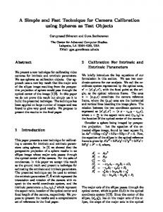
Calibration panel pattern
The calibration pattern, shown in Figure 4, was designed in CAD software. It follows the purposes of trouble-free image point determination, either in manual or auto mode, and to allow a quick perception of the panel orientation in the images, for which reason some reference marks were placed. It was then printed at true scale over a rigid material. Its dimensions are 110cmx150cm.
Figure 5: Estimation of corners positions, based on 8 to 10 points (crosses) indicated by the user. 3. TESTS AND RESULTS
In order to assess its overall performance, the method was tested with two data sets corresponding to cameras with different sensor and lens characteristics. The tests were repeated for each camera considering the following six sets of parameters: Set 1: x0, z0, f Set 2: x0, z0, f, κ1 Set 3: x0, z0, f, κ1, κ2 Set 4: x0, z0, f, λ, κ1, κ2 Set 5: x0, z0, f, λ, k1, k2, p1, p2 Set 6: x0, z0, f, λ, κ1, κ2, κ3, p1, p2 The meaning of the parameters is indicated in (1), (2) and (3). 3.1
Figure 4: Calibration pattern. 2.7
Image coordinate measurement
The pixel coordinates of the pattern corners are extracted automatically. The process has two main stages. Stage 1: The positions of the corners are estimated and enclosed in 10x10 pixels image patches, as shown in Figure 5. In order to make this stage more robust it is requested that the user indicates the pattern corners plus four or six mid points and the number of horizontal and vertical squares. Adapting second or third order polynomial to these points, it is possible to closely estimate the positions of points at the corners of the squares in the pattern.
Test 1
The method was initially tested with a set of images, obtained with a camera whose lens were relatively narrow angle and without obvious geometric distortions. Characteristics of the camera used (AVT Marlin): - ½ inch type CCD array. - Cell size of 8.3μm x 8.3μm - Array size of 780 x 580 pixels. Characteristics of the lens used: - Focal Length: 12mm - Iris range: F1.4 – Close - Minimum Object Distance: 0,1m - Field of view (Horizontal): 29.8º for a ½ inch CCD. The images used to carry out this test are shown in Figure 6.
Stage 2: in each image patch a corner detection algorithm is applied, based on the Sobel operator for edge detection (Sobel, 1978).
Figure 6: Images used for camera calibration in Test 1. The parameters obtained for each test are indicated in Table 2. x0 , z 0 and f are in pixel units and the other parameters are in
normalized units. The number of iterations needed is presented in the first row and the standard deviation of the parameters residuals, in normalized units, are in the last row.
introduced besides the principal point coordinates and focal distance. 3.2
iter x0 z0 f
Set 1 5 400.90 291.08 1549.64
λ κ1 κ2 κ3 p1 p2 std
Set 2 5 402.97 290.63 1548.96
Set 3 5 402.97 290.62 1549.07
0.0324
0.0374 -0.0780
0.370
0.362
0.360
Set 4 6 402.49 290.71 1550.11 0.9995 0.0373 -0.0613
Set 5 6 391.23 292.50 1549.90 0.9995 0.0343 0.0172
0.361
0.0026 -0.0005 0.360
Set 6 8 389.92 292.68 1548.40 0.9995 -0.0634 3.500 -34.46 0.0029 -0.0005 0.359
Table 2 – Estimations of the internal parameters
The correlations between the parameters are presented in Table 3. This test is useful to assess if any set of parameters are highly correlated, which means that one of them is sufficient to include in the model. In Table 3 the highest correlations found are shaded.
z0 f
λ k1 k2 k3 p1 p2
x0 -0.01 -0.02 0.17 0.05 -0.06 0.08 -0.90 0.02
z0
f
λ
0.03 0.00 0.01 -0.01 0.01 0.00 -0.86
-0.17 0.24 -0.24 0.22 0.00 0.02
0.06 -0.07 0.07 -0.10 -0.01
k1
-0.97 0.91 -0.05 -0.01
k2
-0.98 0.06 0.01
k3
-0.08 -0.01
p1
-0.01
Another test consisted in re-projecting the points of the panel to the image planes, using the calculated parameters and analysing the differences to the true positions. The statistic parameters calculated were the maximum, minima and Root Mean Square of the errors (RMSE) in x and z, in pixel coordinates, and, also, the maxima and minimum of the linear errors, in pixels. Results of this test are presented in Table 4. 1 1.88 0.43 1.15 0.29 1.92 0.41
2 1.73 0.43 1.01 0.28 1.81 0.40
3 1.73 0.43 1.01 0.28 1.81 0.40
4 1.75 0.43 0.97 0.28 1.83 0.39
5 1.63 0.42 1.02 0.28 1.71 0.40
The method was also tested with a second set of images, obtained with a camera whose lens were very wide angle and the geometric distortions were more obvious than that of test 1. One of the images obtained with this camera can be seen in Figure 5. Characteristics of the camera used: - ½ inch type CCD array. - Cell size of 5.6μm x 5.6μm - Array size of 640 x 480 pixels. Characteristics of the lens used: - Focal Length: Vario 1.8 – 3.6 mm - Iris range: F1.6 – Close - Minimum Object Distance: 0,2m - Angle of view (Hor): 97º to 53º for a ¼ inch CCD. Results obtained for this test are presented in the same table structure (Table 5, Table 6 and Table 7).
iter x0 z0 f
Set 1 7 339.58 253.44 503.16
λ κ1 κ2 κ3
Table 3 – Correlations obtained between the parameters
Set Max x error RMS x error Max z error RMS z error Max lin error Mean lin error
Test 2
6 1.57 0.42 1.09 0.28 1.67 0.39
Table 4 – Results of re-projection to images (pixels). 3.1.1 Analysis of the results of Test 1: The method performed stably, since the number of iterations was small. Also, the fact that the z scale factor (λ) was very close to 1, indicates that this parameter could be avoided. Results in Table 3 point to the fact that the principal point coordinates and decentering parameters, p1 and p2, are almost dependent, once their correlation is high. So p1 and p2 could be avoided. Table 3 also shows also that the radial distortion parameters are highly correlated, so one would be sufficient to explain the image radial distortion. Finally, the inspection of Table 4 shows that, for this camera, little gain is achieved when calibration parameters were
p1 p2 std
1.3496
Set 2 6 321.79 235.69 500.84
Set 3 6 321.73 235.59 500.97
0.3541
0.3195 0.1200
0.3153
0.3112
Set 4 6 321.66 235.66 500.82 1.0005 0.3194 0.1196
Set 5 6 321.47 236.70 500.80 1.0006 0.3181 0.1175
0.3109
0.0003 0.0020 0.3081
Set 6 6 321.44 236.67 500.53 1.0006 0.2931 0.3274 -0.4769 0.0003 0.0020 0.3077
Table 5 – Estimations of the internal parameters
z0 f
λ k1 k2 k3 p1 p2
x0 0.01 0.02 -0.04 -0.02 0.00 0.00 0.11 -0.04
z0
f
λ
k1
k2
k3
p1
-0.10 0.04 0.06 -0.06 0.05 0.04 0.21
-0.14 0.16 -0.18 0.19 -0.06 0.02
0.04 -0.05 0.05 0.02 0.10
-0.96 0.90 -0.08 0.07
-0.98 0.04 -0.09
-0.02 0.09
0.03
Table 6 – Correlations obtained between the parameters Set Max x error RMS x error Max z error RMS z error Max lin error Mean lin error
1 9.59 1.44 7.25 1.26 12.02 1.38
2 1.07 0.33 1.00 0.27 1.38 0.35
3 1.12 0.33 1.05 0.26 1.32 0.35
4 1.12 0.33 1.07 0.26 1.32 0.35
5 1.11 0.33 0.94 0.25 1.41 0.34
6 1.11 0.33 0.94 0.25 1.41 0.34
Table 7 – Results of re-projection onto images (pixel units).
Results in Table 5 reveal that the method performed well, once the number of iterations was small. As before the z scale factor (λ) is very close to 1, indicating that with this camera it could also be dropped. Also in this case, as seen in Table 6, the radial distortion parameters are highly correlated, so one parameter would be sufficient to explain the image radial distortion.
Finally, the inspection of Table 7 shows that, for this camera, little gain is achieved when calibration parameters were introduced besides the principal point coordinates, focal distance and κ1 radial parameter. So, in this case, the pixel correction model could be given by the following equation: Δr =
κ1 f
2
.r 3
(13)
The division by f 2 is necessary in order to convert normalized values to pixel values, once f is the normalization factor. Although the distortion reaches large values far from image centre it could be modelled only with k1. Figure 7 shows the graphical representation of the radial correction.
5. REFERENCES AND/OR SELECTED BIBLIOGRAPHY
Bouguet, J. and Perona, P., 1998: “Closed-Form Camera Calibration in Dual Space Geometry”. European Conference on Computer Vision, 1998, Freiburg, Germany. Brown, D. C., 1966: “Decentering Distortion of Lenses”. Photogrammetric Engineering, Vol. 32, nº3, pp 444-462.
140 radial correction (pixels)
A small number of calibration parameters are enough to model the image distortions. This is related to the low resolution of cameras used, as typical of MMS. The tests show that the RMSE of the re-projection to the images is, in general, less than half a pixel, which indicates high quality of the model obtained. For this class of low-resolution cameras, there is little to improve in the calibration process. The usefulness of the implemented method was confirmed.
120
Brown, D. C., 1971: “Close Range Camera Calibration”. Photogrammetric Engineering, Vol. 37, nº8, pp 855-866.
100 80
Fraser, C., 1997. Digital camera self calibration, ISPRS Journal of Photogrammetry & Remote Sensing, nº2, pp 149-159.
60 40 20 0 0
100
200
300
400
500
radius (pixels)
Figure 7: Radial correction in pixel units.
4. CONCLUSIONS
The objective of the work presented in this paper was the development of a method to perform the calibration of cameras used in a Mobile Mapping System. In this kind of environment it is regularly needed to change the image sensors or its internal parameters. So the method has to be quick in its implementation, robust and accurate, since it conditions the final absolute accuracy of the MMS. The method developed relies on the approach described by authors such as Heikkila and Silven (1997), Bouguet and Perona (1998) or Zhang (1999), which is a mixture of photogrammetric calibration and self-calibration. The main features of the developed method are the following: - The calibration object used is a flat panel with a printed pattern in which nearly 150 calibration-points could be rigorously obtained. A flat calibration object is easier to produce than a tri-dimensional one. - The user needs to obtain 10 images of the calibration panel, varying the place and the orientation of the camera. - Image coordinates of the calibration points are extracted semi-automatically, with small user intervention. - Initial approximations of the external orientation parameters of the camera are automatically obtained for each image. - The final internal calibration parameters are obtained after an equation system adjustment based on the collinearity equations. The results of the tests made, in order to assess the capabilities of the method, allow for some important conclusions. The method is simple and quick in its operation. The user only has to take the images and indicate, for each image, 8 corner points of the panel. The method performs robustly once, in general, a small number of iterations are sufficient to obtain the results.
Heikkila, J. and Silven, O., 1997: “ A Four Step Camera Calibration Procedure With Implicit Image Correction”. Procedures of the 2nd European Conference on Computer Vision and Pattern Recognition, 1997, pp. 1106-1112, Puerto Rico. Madeira, S., Gonçalves, J. A., Bastos, L., 2007: Implementation of a Low Cost Mobile Mapping System”. Proceedings of The 5th International Symposium on Mobile Mapping Technology, Padua, Italy. Sobel, I., 1978. Neighbourhood Coding of Binary images for Fast Contour Following a General Array Binary Processing, Computer Graphics and Image Processing, vol 8, pp. 127-135. Wolf, P. R. and Dewitt, B. A., 2000. Elements of photogrammetry, with applications in GIS., McGraw-Hill, 3rd Edition, pp. 233-259. Zhang, Z., 1999: “Flexible Camera Calibration by Viewing a Plane From Unknown Orientations”. Proceedings of International Computer Vision Conference, 1999, Vol I, pp. 666-673.