Computerized Medical Imaging and Graphics 29 (2005) 251–258 www.elsevier.com/locate/compmedimag
Fast colon centreline calculation using optimised 3D topological thinning Robert J.T. Sadleir*, Paul F. Whelan Vision Systems Group, School of Electronic Engineering, Dublin City University, Dublin 9, Ireland Received 27 April 2004; revised 18 October 2004; accepted 18 October 2004
Abstract Topological thinning can be used to accurately identify the central path through a computer model of the colon generated using computed tomography colonography. The central path can subsequently be used to simplify the task of navigation within the colon model. Unfortunately standard topological thinning is an extremely inefficient process. We present an optimised version of topological thinning that significantly improves the performance of centreline calculation without compromising the accuracy of the result. This is achieved by using lookup tables to reduce the computational burden associated with the thinning process. q 2004 Elsevier Ltd. All rights reserved. Keywords: Colon; Computed tomography colonography; Centreline; 3D topological thinning; Virtual endoscopy
1. Introduction Virtual reality imaging of the colon using computed tomography (CT) data was originally demonstrated by Vining et al. [1] in 1994. This technique, more recently known as CT Colonography (CTC) [2], is a minimally invasive alternative to conventional colonoscopy for colon imaging. CTC involves generating a computer model of the colon using data obtained from an abdominal CT study of a suitably prepared patient. The resulting virtual colon can be examined in a manner similar to conventional colonoscopy. Unaided endoluminal navigation at CTC is impractical due in part to the tortuous nature of the colon. This problem can be alleviated to some extent by identifying an approximation of the central path through the colon. This path is commonly referred to as the colon centreline. The centreline can subsequently be used to constrain and thus greatly simplify the task of endoluminal navigation. Identifying the centreline of the colon at CTC is not a trivial process. This task is compounded by the shear volume of data contained in a CTC dataset in addition to * Corresponding author. Tel.: C353 1 7008592; fax: C353 1 7005508. E-mail addresses:
[email protected] (R.J.T. Sadleir), paul.
[email protected] (P.F. Whelan). 0895-6111/$ - see front matter q 2004 Elsevier Ltd. All rights reserved. doi:10.1016/j.compmedimag.2004.10.002
the complicated morphology of the colon. Ideally, a centreline calculation algorithm should generate an accurate approximation of the central path through the colon with minimal operator intervention in a reasonable amount of time. The time constraint is especially important considering the potential deployment of such an algorithm in a clinical environment. The problem of centreline calculation has received a great deal of attention since the introduction of CTC and a vast number of centreline calculation algorithms have been described in the literature. These algorithms are briefly summarised and compared (where possible) in Table 1. A number of early centreline calculation algorithms [18,19] were based on a technique known as onion peeling or topological thinning [20]. The use of standard topological thinning for this type of application is considered by many to produce accurate results [3,8,10,11,15], however, it is also regarded as being extremely inefficient [3,7,8,11,12,14,15]. As a result the majority of recently published approaches either describe efficient alternatives to topological thinning or modifications to the standard topological thinning algorithm that increase performance. Ge et al. [13] provide an excellent example of a centreline calculation algorithm based on topological thinning (summarised in Fig. 1). Their multistage algorithm begins by identifying voxels that represent the colon lumen. This process, known as segmentation, is achieved
252
R.J.T. Sadleir, P.F. Whelan / Computerized Medical Imaging and Graphics 29 (2005) 251–258
Table 1 An overview of previously published centreline calculation algorithms Group
Year
Technique
Platform
CPU (MHz)
RAM (Mb)
Time (s)
Wan et al. [3]
2002
Intel
700
655
14.75a
Sadleir and Whelan [4]
2002
Intel
700
512
24.42
Deschamps et al. [5]
2001
Sun/Solaris
300
1024
30
Chen et al [6]
2000
SGI
36
1998 2001
195!2 (R10,000) NA 1000
896
Samara et al. [7] Bitter et al. [8]
NA NA
w60 119
Zhou et al [9]
1998
NA
NA
199
Sato et al [10]
2000
208
2000
194 (R10,000) 194 (R10,000)
NA
Bitter et al [11]
4096
276
Samara et al. [12]
1999
896
w300
Ge et al. [13]
1999
Zhou and Toga [14]
1999
Paik et al. [15]
1998
McFarland et al. [16] Chiou et al. [17]
1997 1999
Minimum cost path through a distance from surface field Optimized 3D topological thinning using Lookup tables Minimum energy path through a distance from source field with a centering potential derived from a distance from surface field Minimal cost path through a distance from source field followed by a centering stage Distance from source field with cluster centering Centerline calculated as minimum cost path from end to start point in a penalized distance field Skeleton extraction using a distance form surface field followed by centerline identification Centerline calculated as minimum cost path from end to start point in a penalized distance field Centerline calculated as minimum cost path from end to start point in a penalized distance field Distance from source field with cluster centering and centerline refinement stage 3D topological thinning used in conjunction with surface voxel tracking Distance from source field with cluster centers used as centerline points A combination of a distance from source field and streamlined 3D topological thinning Radiologist marking & spline interpolation Identify and connect principle attractors, i.e. local maxima in distance from surface field
a b c
SGI Intel/ Windows SGI SGI SGI SGI SGI
NA
NA
518 (60b)
SGI
NA
519
SGI
NA (R10,000) 180 (R5000)
256
759c
NA SGI
NA NA
NA 3072
1080 Exact figure unavailable
Does not include the time required to generate the distance fields (average time of presented results). Obtained by sub sampling the dataset. Includes time required for segmentation stage.
using a simple 3D region growing algorithm. A topological thinning algorithm is subsequently employed to obtain a skeleton representation of the segmented colon lumen. Finally, the centreline is obtained by reducing the skeleton to a single centred path between two user defined endpoints. Optimisation techniques including surface voxel tracking and dataset subsampling are employed to improve performance. Centreline calculation using this approach requires approximately 60 s. Although this is relatively fast it is still significantly slower than more recent alternatives. In this article we describe a fast colon centreline calculation algorithm using an optimised approach to 3D topological thinning. We begin by summarising a standard approach to centreline calculation using topological thinning that is loosely based on the technique described by Ge et al. [13]. Then we outline how the performance of this approach can be significantly improved by employing a lookup-table (LUT) based optimisation technique. Finally, we present the results of our study comparing the performance of these two techniques and comment of the significance of these results before concluding the article.
2. Methods 2.1. Patient preparation and data acquisition Prior to their scheduled examination all patients were instructed to take a low-residue diet for 48 h followed by clear fluids for 24 h. Prior to the day of examination, patients were instructed to take one sachet of Pixcolax at 08.00, a second sachet of Pixcolax at 12.00, a sachet of clean prep in a litre of cold water at 18.00 and a Senokot tablet at 23.00. Immediately before the examination the colon was gently insufflated with room air to the maximum tolerable level and the patient was subsequently scanned in both the supine and prone positions to reduce the effect of residual material in the colon. All scans were obtained using a Siemens Somatom 4, four slice multidetector Spiral CT scanner. The scanning parameters were 120 kVp, 2.5 mm collimation, 3 mm slice thickness, 1.5 mm reconstruction interval, 0.6 s gantry rotation and field of view of 3808. The scanning time ranges from 20 to 30 s, so the acquisition is performed in single breath-hold. The procedure was first performed with the patient in the supine position and then repeated with
R.J.T. Sadleir, P.F. Whelan / Computerized Medical Imaging and Graphics 29 (2005) 251–258
253
Fig. 1. An overview of the centreline calculation process. (a) The original CTC dataset; (b) The segmented colon lumen; (c) The skeleton; (d) The final colon centreline.
the patient in the prone position. The number of slice varies from 250–300 depending on the height of the patient and each slice comprised of 512!512 pixels. Typical total size of the volumetric data is approximately 150 Mb 2.2. Segmentation and endpoint detection The colon lumen is extracted from the CTC dataset using a standard region growing based segmentation technique [21,22]. Segmentation results in a binary model of the colon lumen consisting of only object [1] and background [0] voxels. The two endpoints required for centreline calculation can be automatically identified during the segmentation process using a technique based on distance fields [8]. Any cavities, i.e. background voxels located within the segmented colon lumen, may adversely affect skeleton generation and must be removed. Finally, the volume is cropped to the minimum size required to enclose the entire segmented colon lumen. The resulting solid binary object and endpoint pair constitute the inputs to the centreline calculation algorithm 2.3. Skeleton generation The skeleton of the segmented colon lumen is obtained using topological thinning. The thinning process involves the removal of layers of surface voxels from a binary object. A surface voxel, i.e. one that is not completely
surrounded by other object voxels, is only removed if it does not affect certain structural properties of the object being thinned. These properties describe the object in terms of overall connectivity, holes and endpoints. Layers of surface voxels are removed iteratively and the process terminates when no more surface voxels can be removed without compromising the structural properties outlined above. The resulting set of voxels represents the skeleton of the original object. The initial set of surface voxels are identified by performing a raster scan of the entire volume. Subsequent surface voxels can be identified more easily by examining the six directly connected neighbours of deleted voxels. A total of three tests must be performed prior to the deletion of a particular surface voxel, these tests deal with the following requirements: 1. Endpoint retention: The number and location of endpoints in the skeleton must be the same as in the original object. In the case of centreline calculation there are only two endpoints of interest, these are located in the rectum and caecum. 2. Connectivity preservation: The number of distinct binary objects in the scene must be the same before and after the application of the topological thinning algorithm. 3. Hole prevention: The removal of a surface voxel must not introduce a new hole into the object being thinned.
254
R.J.T. Sadleir, P.F. Whelan / Computerized Medical Imaging and Graphics 29 (2005) 251–258
If the deletion of a particular surface voxel respects all of these requirements then it is removed otherwise it is retained possibly to be deleted at a subsequent iteration. The endpoint retention test is trivial and involves comparing the coordinates of the voxel under examination with those of the two predefined endpoints. The other two tests, connectivity preservation and hole prevention, are much more complicated and require a significant amount time to perform. In each of these cases the test involves extensively examining the configuration of the 26 voxels in the 3!3!3 region surrounding the deletion candidate. 2.4. Skeleton reduction (centreline generation) The skeleton that results from the topological thinning stage incorporates the colon centreline. Unfortunately, it also includes a number of extraneous loops that occur due to holes in the original segmented colon lumen (see Fig. 2(a)). These holes are a common occurrence usually associated with the Haustral folds. The skeleton branches caused by holes are closer to the surface of the colon than those associated with the actual centreline. The proximity of a particular skeleton voxel to the original surface is related to the thinning iteration at which that voxel was uncovered. By assigning the relevant thinning index to each voxel as it is exposed it is possible to generate a distance field that represents the approximate distance of each lumen voxel from the colon surface. Following an inversion of the distance values it is possible to generate a weighted graph where the centreline can be identified as the minimum cost path between the two predefined endpoints. The minimum
cost path can be found in an extremely efficient manner using a simplified version of the Dijkstra shortest path algorithm [23]. The resulting set of points represents the final centreline, i.e. the path between the two predefined endpoints that is furthest from the surface of the original segmented colon lumen (see Fig. 2(b)). The skeleton reduction process is illustrated in Fig. 3 using a 2D example. 2.5. Optimisation The method for centreline calculation outlined in the previous paragraphs forms the basis for our optimised implementation and will be used as a standard for comparison purposes. Our enhancements deal specifically with the skeleton generation stage, particularly the tests for connectivity preservation and hole prevention. Both of these tests must be performed repeatedly, at least once for each object voxel, and represent the most time consuming aspect of the centreline calculation process. In each case the 3!3!3 neighbourhood surrounding the voxel under examination is extensively analysed in order establish whether its removal will affect the relevant global properties of the object, i.e. overall connectivity and number of holes. The result of this analysis is dependant on the values of the 26 neighbours surrounding the voxel under examination. Each of these voxels can belong to one of two classes, either object or background, consequently the number of possible neighbourhood configurations is 67,108,864 (226). In order to streamline the centreline calculation process we generate all possible neighbourhood configurations. Each neighbourhood is tested for connectivity preservation
Fig. 2. Magnified sections of the colon lumen from Fig. 1 illustrating how extraneous loops can be caused by the Haustral fold (a) and how the removal of the these loops yields the final centreline (b).
R.J.T. Sadleir, P.F. Whelan / Computerized Medical Imaging and Graphics 29 (2005) 251–258
255
Fig. 3. A 2D example illustrating the skeleton reduction process. (a) Original binary object (region of interest indicated using white); (b) skeleton and distance from surface field generation; (c) inverted distance from surface field (skeleton pixels only); (d) weighted graph (originating from the right); (e) the minimum cost path found using backward propagation through the distance field.
and hole prevention. The results of these tests are combined into a single pass/fail binary value and stored in a LUT structure. Each result is addressed by a unique index, I, that is obtained by multiplying the value of each voxel in the neighbourhood (V0KV25) with a weight in the range 20–225 and then summing the results:
IZ
25 X
2n V n
using the technique described earlier to obtain the final centreline. It is extremely important to note that the LUT is calculated only once. It is subsequently stored in a file on the hard disk and reloaded (not recalculated) each time it is
(1)
nZ0
This is essentially a 3D convolution operation where the value of the central voxel is not used in the calculation. A simplified 2D example of the index generation process is illustrated in Fig. 4. The LUT can subsequently be used to streamline the standard centreline calculation algorithm. During the thinning phase of the algorithm, the computationally intensive tests for connectivity preservation and hole prevention are no longer necessary. Instead, the relevant index is quickly generated using the equation above and the LUT is queried to determine whether or not the central voxel can be removed. The thinning process continues until only skeleton voxels remain and the skeleton is reduced
Fig. 4. A 2D illustration of the LUT index generation process.
256
R.J.T. Sadleir, P.F. Whelan / Computerized Medical Imaging and Graphics 29 (2005) 251–258
Fig. 5. Examples of centreline calculation where segmented yielded a single hollow tube connecting the rectum to the caecum.
required for centreline calculation. The time required the load the LUT is significantly less than the time required to generate it.
3. Results We evaluated both the standard and optimised centreline calculation algorithms using 12 CTC datasets (6 prone and 6 supine) that were acquired from our CTC database. Only datasets with intact colons, i.e. colons without collapse or extreme blockage, were selected. Examples of the centreline obtained are illustrated in Fig. 5. Both techniques produced perfectly matching centrelines in all cases. The comparison was performed by calculating the distance from each voxel in the optimised centreline with the nearest pixel in the standard centreline. In all cases the sum of these distances was zero. The average time required for centreline calculation using the standard approach was 155.413 s compared to 3.438 s for the optimised approach (see Table 2 for a detailed breakdown of results). The once off task of lookup table initialisation required approximately 1.5 h. However, loading the table prior to each centreline calculation required less than 1 s. All software was implemented using the Java 2 standard edition version 1.4.2 (Sun Microsystems Inc., Santa Clara, CA, USA) and tested on a standard PC workstation (1.6 GHz CPU and 512 Mb RAM) running Microsoft Windows XP professional (Microsoft Corp., Redmond, WA, USA). Note that similar results were obtained using a CCC implementation of our optimised centreline calculation algorithm running on the same hardware platform.
4. Discussion Centreline calculation using standard topological thinning is an extremely time consuming process. We have described how the performance of topological thinning can be improved by utilising a LUT to significantly reduce demand on the CPU. We have demonstrated how our optimised approach outperforms standard topological thinning based centreline calculation with execution times that are an average of 45 times faster that the standard approach. Our modifications are relatively straightforward to Table 2 Detailed results comparing the standard and optimised approaches to centreline calculation
Patient position Dataset size (slices) Lumen size (voxels) Ratio of centreline/ skeleton voxels Loading LUT (s) Loading cropped dataset (s) Surface detection (s) Skeleton generation (s) Skeleton reduction (s) Overall with optimisation t1 (s) Overall with out optimisation t2 (s) Improvement (t2/t1)
Dataset A (best case)
Dataset B (worst case)
Average (all 12 datasets)
Prone 253 2,027,478 0.536
Supine 257 3,473,202 0.398
– 272 2,106,836 0.617
0.844 0.844
0.86 1.859
0.834 1.409
0.187 0.734 0.141 2.75
0.359 1.563 0.047 4.688
0.279 0.844 0.066 3.438
147.453
256.015
155.413
53.619
54.611
44.995
Our optimisation technique only affected the skeleton generation stage of the centreline calculation process. The time required for all other stages remained the same as the unoptimised approach.
R.J.T. Sadleir, P.F. Whelan / Computerized Medical Imaging and Graphics 29 (2005) 251–258
257
Fig. 6. Examples of centreline calculation where the colon is represented by multiple segments (a) blockage in the descending colon and (b) blockage at the splenic flexure.
implement and do not alter the core functionality of the topological thinning algorithm, hence the quality of the resulting centreline is not compromised. The only time consuming aspect of our approach is the task of lookup table population. This requires extensively analysing over 67 million neighbourhoods and requires several hours to complete. Fortunately once generated the same lookup table can be used for all subsequent centreline calculations. The centreline calculation technique described in this paper deals with intact colons, i.e. colons where there is an unobstructed path between the rectum and the ceacum. Consequently this technique is not restricted to applications in CTC and can be used in other areas of virtual endoscopy where a single path or even multiple flight paths are required for a hollow object. In the case of colons with collapsed segments or extreme blockages, segmentation of the colon will yield a number of subsections that represent the air filled colon lumen. Here the centreline calculation algorithm must be applied to each of the individual sections and the centreline segments can then be combined to yield the final result. Dealing with the problem of collapsed and blocked colons falls into the realm of segmentation and a method developed by our group for automatic segmentation of collapsed and blocked colons is the subject of another paper (currently under review elsewhere—reference provided when available). Fig. 6 provides some examples of how our centreline calculation algorithm can be used in cases where colon segmentation yields multiple segments.
5. Summary We have introduced an optimised version of topological thinning that significantly reduces the computational
overhead associated with skeleton generation. Our novel approach to thinning streamlines the entire centreline calculation process without compromising the accuracy of the outcome. The technique itself is quite simple and straightforward to implement, however, the performance represents a major improvement over the standard approach being on average 45 times faster.
Acknowledgements The authors would like to thank Dr Helen Fenlon and Dr John Bruzzi from the Department of Radiology at the Mater Misercordiae Hospital, Dublin, Ireland for supplying the CTC datasets used in this study. We would also like to thank Tarik Chowdhury of the Vision Systems Group for providing the images that illustrate how our documented centreline calculation algorithm can be used with collapsed and blocked colons.
References [1] Vining DJ, Gelfand DW, Bechtold RE, Scharling ES, Grishaw EK, Shifrin RY. Technical feasibility of colon imaging with helical CT and virtual reality. AJR 1994;162(S):104. [2] Johnson CD, Hara AK, Reed JE. Virtual endoscopy: what’s in a name? AJR 1998;171(5):1201–2. [3] Wan M, Liang Z, Ke Q, Hong L, Bitter I, Kaufman A. Automatic centerline extraction for virtual colonoscopy. IEEE Trans Med Imaging 2002;21(12):1450–60. [4] Sadleir RJT, Whelan PF. Colon centreline calculation for CT colonography using optimised 3D topological thinning. In: First International Symposium on 3D Data Processing, Visualization and Transmission, 2002;800–3.
258
R.J.T. Sadleir, P.F. Whelan / Computerized Medical Imaging and Graphics 29 (2005) 251–258
[5] Deschamps T, Cohen LD. Fast extraction of minimal paths in 3D images and applications to virtual endoscopy. Med Image Anal 2001; 5(4):281–99. [6] Chen D, Li B, Liang Z, Wan M, Kaufman AE, Wax M. Tree-branch searching multiresolution approach to skeletonization for virtual endoscopy. Proc SPIE Med Imaging: Image Process 2000;3979: 726–34. [7] Samara Y, Fiebich M, Dachman AH, Doi K, Hoffmann KR. Automated centreline tracking of the human colon. Proc SPIE Med Imaging: Image Process 1998;3338:740–6. [8] Bitter I, Kaufman AE, Sato M. Penalized-distance volumetric skeleton algorithm. IEEE Trans Vis Comp Graph 2001;7(3):195–206. [9] Zhou Y, Kaufman A, Toga AW. Three-dimensional skeleton and centerline generation based on an approximate minimum distance field. Vis Comput 1998;14(7):303–14. [10] Sato M, Bitter I, Bender M, Kaufman A, Nakajima M. TEASAR: treestructure extraction algorithm for accurate and robust skeletons. Proc Pacific Graph 2000;281–9. [11] Bitter I, Sato M, Bender M, McDonnell KT, Kaufman A, Wan M. CEASAR: a smooth, accurate and robust centreline extraction algorithm. Proc IEEE Visualisation 2000;45–52. [12] Samara Y, Fiebich M, Dachman AH, Kuniyoshi JK, Doi K, Hoffmann KR. Automated calculation of the centerline of the human colon on CT images. Acad Radiol 1999;6(6):352–9. [13] Ge Y, Stelts DR, Wang J, Vining DJ. Computing the centerline of a colon: a robust and efficient method based on 3D skeletons. J Comput Assist Tomogr 1999;23(5):786–94. [14] Zhou Y, Toga AW. Efficient skeletonization of volumetric objects. IEEE Trans Vis Comp Graph 1999;5(3):196–209. [15] Paik DS, Beaulieu CF, Jeffrey RB, Rubin GD, Napel S. Automated flight path planning for virtual endoscopy. Med Phys 1998;25(5): 629–37. [16] McFarland EG, Wang G, Brink JA, Balfe DM, Heiken JP, Vannier MW. Spiral computer tomographic colonography: determination of the central axis and digital unravelling of the colon. Acad Radiol 1997;4(5):367–73. [17] Chiou RCH, Kaufman AE, Liang ZR, Hong LC, Achniotou M. An interactive fly-path planning using potential fields and cell decomposition for virtual endoscopy. IEEE Trans Nuc Sci 1999;46(4):1045–9. [18] Hong L, Kaufman A, Wei YC, Viswambharan A, Wax M, Liang Z, Loew M, Gershon N. 3D virtual colonoscopy. Proc IEEE Biomed Visualisation Symp 1995;26–32. [19] Ge Y, Stelts DR, Wang J, Vining DJ. Computing the central path of the colon from CT images. Proc SPIE Med Imaging: Image Process 1998;3338:702–13. [20] Tsao YF, Fu KS. A parallel thinning algorithm for 3-D pictures. Comput Graph Image Proc 1981;17:315–31. [21] Sato M, Lakare S, Wan M, Kaufman A, Wax M. An automatic colon segmentation for 3D virtual colonoscopy. IECE Trans Inf Syst 2000; E84(1):201–8. [22] Wyatt CL, Ge Y, Vining DJ. Automatic segmentation of the colon for virtual colonoscopy. Comput Med Imaging Graph 2000;24(1):1–9. [23] Dijkstra EW. A note on two problems in connexion with graphs. Numer Math 1959;1:269–71.
Robert Sadleir received his B. Eng. (Hons) degree in Electronic Engineering from Dublin City University (DCU) in 1998. Immediately after completing his degree Mr Sadleir was employed as a consultant software developer by the Vision Systems Laboratory at DCU. This work culminated in the release of the NeatVision software development environment. Mr Sadleir subsequently resumed employment at 3Com technologies Ireland Ltd. where he worked for a period during his undergraduate studies. At 3Com he worked as an Application Specific Integrated Circuit (ASIC) development engineer and was involved in the development of Ethernet switching products. Mr Sadleir returned to DCU in 1999 where he is employed as a lecturer in the School of Electronic Engineering. Mr Sadleir is currently completing his PhD in the area of medical image analysis at DCU. His PhD research deals with CT dataset analysis for automatically detecting colorectal cancer. This work has received funding from the Irish Cancer Society, the Health Research Board and Science Foundation Ireland. Mr Sadleir has published in a wide range of areas including engineering, radiology and gastroenterology. Additionally he has been invited to speak at the International Workshop on Multislice CT, 3D Imaging and Virtual Endoscopy in 2002 and again in 2003. His research is primarily focused in the area of virtual colonoscopy; however, he is also involved in research dealing with DICOM and remote access education. Mr Sadleir is a member of the International Association for Pattern Recognition (IAPR), the Irish Pattern Recognition and Classification Society (IPRCS) and the Institution of Engineers of Ireland (IEI).
Prof. Paul F Whelan received his B. Eng. (Hons) degree from the National Institute for Higher Education Dublin, a M. Eng. degree from the University of Limerick, and his PhD (Computer Science) from the University of Wales, Cardiff. During the period 1985–1990, he was employed by Industrial and Scientific Imaging Ltd and later Westinghouse (WESL), where he was involved in the research and development of industrial vision systems. He was appointed to the School of Electronic Engineering, Dublin City University (DCU) in 1990 and currently holds the position of Associate Professor. Prof. Whelan found the Vision Systems Laboratory and its associated Vision Systems Group (VSG) in 1990 and currently serves as its director. As well as publishing over 90 peer reviewed papers, Prof. Whelan has published 3 including Selected Papers on Industrial Machine Vision Systems (SPIE-1994), Intelligent Vision Systems for Industry (Springer-1997) and Machine Vision Algorithms in Java (Springer-2000). His research interests include image segmentation (specifically morphology, texture analysis) with applications in computer vision and medical imaging. He is a Senior Member of the IEEE (and the DCU IEEE student branch counsellor), a Chartered Engineer and a member of the IEE and IAPR. He is also a member of a range of computer vision related conference program committees and acts as a reviewer for a number of the main computer vision journals. He served on the IEE Irish centre committee (1999–2002) and is member of the governing board of the International Association for Pattern Recognition (IAPR) and the current President of the Irish Pattern Recognition and Classification Society (IPRCS). Prof. Whelan is an SFI funded principal investigator. See www.eeng.dcu.ie/~vsl for additional details on his work.