Fast Compression of Large Semantic Web Data ... - Semantic Scholar

IEEE TRANSACTIONS ON PARALLEL AND DISTRIBUTED SYSTEMS, VOL. X, NO. X, 201X

1

Fast Compression of Large Semantic Web Data using X10 Long Cheng, Avinash Malik, Spyros Kotoulas, Tomas E Ward, Senior Member, IEEE, and Georgios Theodoropoulos Abstract—The Semantic Web comprises enormous volumes of semi-structured data elements. For interoperability, these elements are represented by long strings. Such representations are not efficient for the purposes of applications that perform computations over large volumes of such information. A common approach to alleviate this problem is through the use of compression methods that produce more compact representations of the data. The use of dictionary encoding is particularly prevalent in Semantic Web database systems for this purpose. However, centralized implementations present performance bottlenecks, giving rise to the need for scalable, efficient distributed encoding schemes. In this paper, we propose an efficient algorithm for fast encoding large Semantic Web data. Specially, we present the detailed implementation of our approach based on the state-of-art asynchronous partitioned global address space (APGAS) parallel programming model. We evaluate performance on a cluster of up to 384 cores and datasets of up to 11 billion triples (1.9 TB). Compared to the state-of-art approach, we demonstrate a speed-up of 2.6 − 7.4× and excellent scalability. In the meantime, these results also illustrate the significant potential of the APGAS model for efficient implementation of dictionary encoding and contributes to the engineering of more efficient, larger scale Semantic Web applications. Index Terms—RDF; parallel compression; dictionary encoding; X10; HPC

F

1

I NTRODUCTION

T

HE Semantic Web possesses a number of significant advantages over the traditional web, such as amenability to machine processing, information lookup and knowledge inference. This model of the web is founded on the concept of Linked Data [1], a term used to describe the practices of exposing, sharing and connecting information on the web using recent W3C specifications such as RDF and URIs. As Linked Data increasingly exposes data from multiple domains, such as general knowledge (DBpedia [2]), bioinformatics (Uniprot [3]), and GIS (linkedgeodata [4]), the potential for new knowledge synthesis and discovery increases immensely. Capitalizing on this potential requires Semantic Web applications which are capable of integrating the information available from this rapidly expanding web. This web is build on the W3C’s Resource Description Framework (RDF) [5] - a schema-less, graph-based data format which describes the Linked Data model in the form of subject-predicate-object (SPO) expressions based on statements of resources and their relationships. These expressions are known as RDF triples. As an example, the simple statement from DBpedia (, , )

• • • • •

L. Cheng is with the Faculty of Computer Science, TU Dresden, Germany. E-mail: [email protected] A. Malik is with the Dept. Electrical & Computer Engineering, University of Auckland, New Zealand. E-mail: [email protected] S. Kotoulas is with the IBM Research, Dublin, Ireland. E-mail: [email protected] TE. Ward is with the Dept. Electronic Engineering, National University of Ireland Maynooth, Ireland. E-mail: [email protected] G. Theodoropoulos is with the Institute of Advanced Research Computing, Durham University, UK. E-mail: [email protected]

conveys the information that the corporation IBM was founded in New York. The Semantic Web already contains billions of such statements and this number is growing rapidly. As the terms in an RDF statement consist of long string characters in the form of either URIs or literals, storing and retrieving such information directly on an underlying database, namely a triple store, will result in (1) unnecessarily high disk-space consumption and (2) poor query performance (querying on strings is computationally intensive). Dictionary encoding has been shown to be an efficient way to ameliorate these problems. Using dictionary encoding all the terms are replaced by numerical ids through a mapping dictionary, and all the original triples are finally converted to id triples before storing. The conventional encoding approach is that all the terms retrieve their ids through sequential access of a single dictionary an approach which is easy to implement but not suitable for compressing large data sets due to time of execution and memory requirements. Consequently, encoding triples in parallel based on a distributed architecture with multiple dictionaries, becomes an attractive choice for this problem. While many approaches focus on data compression ratios or corresponding query performance, in this work, we instead establish the following two performance goals: (1) Large data - our target is to encode (i.e. compress) huge RDF datasets, so as to meet the big data challenges from large data warehouses and the Semantic Web. (2) Fast speed - we focus on achieving high throughput performance, so that the encoded data can undergo further downstream processing as quickly as possible. To achieve these targets we developed a custom encoding algorithm for massive RDF datasets. The approach is implemented using the Asynchronous Partitioned Global


Address Space (APGAS) model programming language X10 [6], and we conduct a performance evaluation on an experimental configuration consisting up to 384 cores (32 nodes) and datasets comprising of up to 11 billion triples (1.9 TB). We summarize our contributions as follows: •

•

•

•

We analyse the challenges of dictionary encoding of large-scale RDF data over a distributed system, and discuss the possible performance issues of current methods. We present a very efficient approach to encoding large RDF datasets. The algorithm is easy on implementation and has obvious performance advantages compared to the state-of-art-method [7]. We describe a detailed implementation of our algorithm using the latest parallel programming language X10, and propose several optimization steps. We also give a brief theoretical analysis of the proposed implementation. We conduct an extensive evaluation of our approach and compare its performance with the state-of-theart. The results demonstrate that our implementation is faster (by a factor of 2.6 to 7.4), can deal with incremental updates in an efficient manner and supports both disk and in-memory processing.

This paper builds upon our earlier work [8]. Here, we introduce four new innovations: (a) We provide a detailed analysis of challenges inherent in massive RDF data encoding and use this to explain the shortcomings in the current state-of-the-art. (b) We conduct a more detailed comparison between our approach and state-of-the-art including a theoretical analysis. (c) We present a detailed version of our algorithm using X10 and present its scalability performance versus input dataset size and number of computation cores based a theoretical analysis. (d) We conduct a more detailed analysis of our experimental results. The rest of this paper is organized as follows: Section 2 provides a review of related work including the details of the state-of-art method. Section 3 presents the challenges of distributed implementation of RDF dictionary encoding. Section 4 introduces the proposed RDF compression algorithm and Section 5 gives the detailed implementation using X10. Section 6 discusses optimizations and improvements to the implementation. Section 7 describes the experimental framework while Section 8 provides a quantitative evaluation of the algorithm. Section 9 concludes the paper.

2

R ELATED W ORK

Compression Approaches. Compression has been extensively studied in various database systems, and has been considered as an effective way to reduce the data footprint and improve overall query processing performance [9] [10]. In terms of efficient storage and retrieval of RDF data, the techniques of data compression have been widely applied to the Semantic Web. Fernández et al. [11] show that universal compression methods (like gzip) can achieve a high compression, due to the structured graph nature of RDF data. Lee et al. [12] present an even more efficient compression scheme for URI references and achieve an improvement of between 19.5 and 39.5% over traditional methods. Weaver

2

et al. [13] propose a syntax for RDF called Sterno and shows that Sterno documents can achieve a compression ratio of under 50%. These methods are geared toward efficient storage and transfer, as opposed to having direct access to the data for efficient processing. To enable RDF triples to be efficiently accessed without prior decompression, various compression approaches have been proposed as well. Yuan et al. [14] try to reduce the storage overhead of common prefixes in IRIs by splitting them based on the last occurrence of ‘/‘ character. In this case, the same prefix appears in all IRIs will be stored only once. Bazoobandi et al. [15] further exploits the high degree of similarity between RDF terms and compress the common prefixes with a variation of a Trie. Moreover, Fernández et al. [16] propose a solution called HDT, which is a binary serialization format optimized for RDF storage and transmission. All these methods are shown to be able to efficiently reduce memory consumption without compromising significantly the encoding and decoding speed for large datasets. However, all these designs focus on singlemachine implementation and lack in scalability. A MapReduce-based implementation of HDT [17] has been proposed recently. This work focuses on building an HDT serialization in a MapReduce environment, as opposed to the encoding scalability issue we address in this work. Dictionary Encoding. Compared to above compression techniques, we focus on dictionary encoding in this work. The reason is that this approach is widely used in current systems. Not only for RDF stores, like Jena [18], Sesame [19], RDF-3X [20] and Virtuso [21] etc., but also in existing DBMS, such as Oracle [22], MonetDB [23] etc. However, to the best of our knowledge, all existing solutions are still based on single node implementation and do not avail of the potential speed-up possible through parallel implementations. In the meantime, though various distributed solutions used to manage RDF data have been proposed in the literature [24] [25] and [26], their main focus is on data distribution after all the statements have been encoded. Currently, there exist only two methods focusing on parallel dictionary encoding of RDF data. One is based on parallel hashing [27] and the other uses the MapReduce framework [7]. Goodman et al. [27] adapt the linear probing method on their Cray XMT machine and realize parallel encoding on a single dictionary through parallel hashing, exploiting specialized primitives of the Cray XMT. Their evaluation has shown that their method is highly efficient and the runtime is linear with the number of used cores. This method requires that all data is kept in memory and is deeply reliant on the shared memory architecture of the Cray XMT, making it unsuitable for distributed memory systems using commodity hardware. They report an improvement of 2.4 to 3.3 compared to the MapReduce system on an inmemory configuration. By comparison, on similar datasets, our approach, as we will see, outperforms the MapReduce system by a factor of 2.6 to 7.4, both on-disk and in-memory. Compared with [27], the method proposed by Urbani et al. [7] is more general that it can be run on ordinary clusters and on-disk. As such, we consider this the stateof-the-art method. The main workflow of the approach is: (a) all the statements are parsed into terms, the popular


3

terms are extracted by sampling the whole data set and their responsible term-id mappings are broadcast to all the computation nodes, (b) the rest non-popular terms is hashredistributed and identifiers are assigned remotely, and (c) the ids of the non-popular terms are redistributed based on their locality information to re-construe the final encoded statements. This approach [7] presents an efficient way to processes high-popularity terms as the ids of these terms can be assigned locally at each node after the broadcasting. This dramatically improves load balancing and speeds up computation. The method has been implemented over MapReduce [28] and the evaluation has shown that the approach scales very well. Regardless, as we will show in Section 3, there still exists possible issues for this method. Moreover, our new proposed approach is approved to be faster than [7], from both theoretical and experimental aspect.

puting and programming language communities (e.g. X10 workshop at PLDI). In the later sections, we will present the detailed implementation of our approach based on X10 and provide the detailed experimental evaluations and analysis to this state of art APGAS-based language. We will also summarize the advantages of this language based on our own development experience in the hope that the big dataanalytics community would consider X10 as a viable choice in their next big project.

Programming Systems. To support parallel and distributed applications, various parallel programming languages and paradigms have been developed by the high performance community. MPI [30] and OpenMP [31] are the most common distributed memory and shared memory parallel execution techniques. More recently, Partitioned Global Address Space (PGAS) based parallel programming languages such as Chapel [32], Unified Parallel C [33], and X10 [6], etc, have witnessed an increasing in adoption, due to the higher level of programming approach compared to MPI and OpenMP. Moreover, X10 in particular enables extraction of shared memory and distributed memory parallelism, while also providing type safety. Similarly, the large scale data-analytics community has developed its own set of parallel processing paradigms. For example, the most popular ones include MapReduce [28] and the lately Spark [34]. Moreover, to support ad-hoc data access, various key-value stores such as HBase [35] Cassandra [36] and Redis [37] have been designed. It is obvious that implementing an application using different languages and systems mentioned above would lead to different application execution times. Regardless, we argue that the technique for parallel execution rather than the language or library used for implementation is more important and the key contribution of this paper. For example, for the RDF compression application, as we will shown in Section 3.2, a simple hash-based dictionary encoding approach would always bring in poor loadbalancing and heavy network communication, irrespective of the underlying implementation system. In such a scenario, a pure performance comparison between the underlying implementation technology used is meaningless. Our focus is on the new methodology letting the designer choose the underlying implementation engine that fulfills their requirements. In this work, based on our own requirements, we have chosen the X10 programming language for implementation purposes1 . X10 has been developed for more than 10 years and has been widely studied in high performance com-

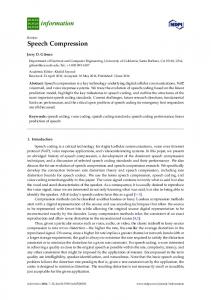
In the environment we are considering, RDF data is partitioned and then compressed using a dictionary on each computation node. However, under this model there exist three main challenges: Challenge 1. Consistency - a term appearing on different compute nodes should have the same id. Both in space and time, the mapping of a term must always maintain its uniqueness. For example, once the term “dbpedia:IBM” is first encoded as id “101” on node A, when encoding this string on another node B, we should also use the same value “101”. Hash functions are potentially useful, but the length of the hash required to avoid collisions when processing billions to terms makes the space cost prohibitive. Challenge 2. Performance - ensuring consistency based on naive methods can lead to serious performance degradation. We can ensure the consistency of the compression in the above example by copying the mapping [dbpedia:IBM, 101] from node A to node B, but network communication cost and dealing with concurrency (e.g. locking on data structures) would lead to poor performance. Challenge 3. Load balancing - the heavy skew of terms may lead to hotspots for the nodes responsible for encoding these popular terms. Compared with the two issues above, load balancing presents a bigger challenge as the distribution of terms in the Semantic Web is highly skewed [39]. To illustrate this skew, we have computed the distribution of the number of a term appears for two real RDF datasets: BTC2011 [29] and Uniprot [3], which contain 2.2 billion and 6.1 billion statements respectively2 . The statistic information of a term appears is demonstrated in Figure 1. It can be seen that there exist both popular (e.g. predefined RDF and RDFS vocabulary) and unpopular terms (e.g. identifiers for entities that only appear for a limited number of times) in both datasets. For a distributed system, like ours, any compression algorithm needs to be carefully engineered so that good network communication and computational loadbalance are achieved. If terms are assigned using a simple hash distribution algorithm, the continuous re-distribution of all the terms would undoubtedly lead to an overloaded network. Furthermore, popular terms would lead to loadbalancing issues.

1. Actually, during the development of a real RDF engine [38], we have found that X10 is a good candidate for programming complex systems. In comparsion, programming a HPC-based query engine using MPI is extremely hard.

3

C HALLENGES

In this section, we first list the challenges of distributed dictionary encoding of RDF data. Then, we discuss the possible performance issues of the state-of-art and outline the key research challenges addressed in this work. 3.1

Challenges on Distributed Systems

2. The details information of the two datasets see Section 7.2

1 0

8

1 0

9

7

1 0

8

1 0

7

6

1 0 1 0

6

1 0

5

1 0

4

1 0

3

1 0

2

1 0

1

1 0 5

1 0 1 0

4

1 0

3

1 0

2

1 0

1

1 0

0

1 0

T h e n u m b e r o f d iffe r e n t te r m s

T h e n u m b e r o f d iffe r e n t te r m s


-1 -1

1 0

0

1 0

1

1 0

2

1 0

3

1 0

4

T h e n u m b e r a te rm

1 0

5

1 0

6

1 0

7

1 0

8

1 0

9

0

1 0 1 0

1 0

4

-1

1 0

-1

1 0

0

1 0

1

1 0

2

1 0

3

1 0

4

T h e n u m b e r a te rm

a p p e a rs

1 0

5

1 0

6

1 0

7

1 0

8

1 0

9

a p p e a rs

Fig. 1. The distribution of the number a term appears of two large RDF datasets (BTC2011 [29] and Uniprot [3]). The horizon-axis means the number a term appears and the vertical-axis means the number of different terms for a given appear time. For example, there are 763 different terms that appear 1000 times for the BTC2011 dataset (left).

Thus, the ratio of skewed terms on the hot nodes over the number of terms on a non-hot node, namely the value of the load-imbalancing factor L1 , is

TABLE 1 Table of notations Notation T |T | n x h x m Wi Ni Li π

3.2

Meaning

xh + xm

(2) L1 = 1 + n · a RDF dataset 1 − (xh + xm ) the number of terms in T the number of computing nodes in the system If the high- and med-popular terms dominate about 1% the portion of high-popular terms in T of T and n is 100, then L1 will be about 2, which means the portion of mid-popular terms in T number of to be encoded terms on each node for the i-th algorithm that there will exist obvious load-imbalancing during the the number of transferred terms for the i-th algorithm encoding implementation. the load imbalancing factor for the i-th algorithm The state-of-the-art MapReduce-based approach [7] uses the duplicate-removing projection operator

Analysis of Current Approaches

For the sake of explanation, let us categorize terms into three groups: high-popularity terms that appear highly frequently, medium-popularity terms that appear a moderate times and low-popularity terms that appear less than a handful of times. For example, for the datasets demonstrated in Figure 3, based on a threshold, we can assume that a term appears more than 10000 times is as considered highpopularity, appears less than 100 as low-popularity and the rest as medium-popularity. As a typical dictionary encoding process includes three main phases: transfer terms to remote nodes, create termid mappings and transfer the mappings back. For simplification, here we just focus on the first phase and track the number of transferred/received terms, as this metric gives the insight into the workloads and network communication. For example, the larger the number of to be encoded terms a node receives, the greater the associated workload will be. In addition, we assume that the skew of the high- and midpopular terms are evenly distributed and the low-popularity terms is uniform distributed. For convenience, we use the notations in Table 1. For a simple hash redistribution method, all the terms of T are redistributed to all the nodes, therefore the number of transferred terms N1 and the number of received terms on each node of W1 will roughly be:

N1 = |T | ( W1 =

an efficient way to process the high popular terms. In that case, large number of these terms will not be redistributed at all, instead, just a small number of pre-defined termid mappings3 π(xh |T |) are broadcast. In the meantime, other terms are hash redistributed as usual4 . Therefore, the number of transferred terms N2 of the approach [7] is:

N2 = n · π(xh |T |) + xm |T | + (1 − xh − xm )|T |

(3)

Moreover, the broadcast mappings do not need to be encoded, and the mid- and low-popular terms are hash redistributed as usual, therefore, after the term transferring that we have the number of terms to be encoded on each node W2 is: ( m )|T | (hot nodes) xm |T | + (1−xh −x n W2 = (1−xh −xm )|T | n

(non-hot nodes)

Compared to the hash-based method, we can see that the network communication is highly reduced because the number each high-popular term appears (e.g. 20000 times) is much greater than n and consequently there is n · π(xh |T |) xh |T |. In the meantime, we have the loadimblancing factor L2 for the MapReduce-based method: xm L2 = 1 + n · (4) 1 − (xh + xm ) Here we have that L2 < L1 , which means that the method [7] can also improve the load-imbalancing problem, compared with a simple hash method. However,

(1)

xh |T | + xm |T | + (1−xh −xm )|T | n

(1−xh −xm )|T | n

(hot nodes) (non-hot nodes)

3. For simplification, we treat a mapping as a term here. 4. In fact, a term with its detailed locality information in the form of are hash redistributed. Here we also choose the term for simplification.


the load balancing problem still exists. The reason is that the medium-popular terms are still based on hashredistribution. Moreover, we argue that for a very large-scale system (n is large), the load imbalancing of the MapReduce-based approach could be obvious. The reason is that the number of low-popular terms is much greater than the high-popular terms (i.e. xm xh ), which we can observe from the cases shown in Figure 3. In fact, we can decrease the threshold for high-popular terms so as to decrease xm and consequently to reduce the load imbalancing. However, in this case, the network communication cost could increase sharply and consequently impact the encoding performance. The reason is that the broadcast operation in a distributed system is always time cost and the broadcast data π(xh |T |) in [7] will highly increase with decreasing xm . For instance, for the BTC2011 dataset, 789835 additional mappings will be broadcast when decreasing the threshold from 10000 to 1000. This means that there is a trade-off between the network communication and load-balancing for the approach presented in [7]. As this trade-off is highly related to the definition of high/mid popularity of terms, then the question is becoming to: to achieve the best performance in large-scale scenarios, How can we reconcile efficient encoding of popular and non-popular terms?

4

FAST D ICTIONARY E NCODING OF RDF DATA

Based on the above research question, in this section, we propose and describe the details of our RDF dictionary encoding approach. Then, we discuss its advantages and compare it with the state-of-the-art. 4.1

Our Approach

Consider the following eight RDF statements, using a simplified notation for terms in the interest of conciseness: , , , , , , ,

We utilise a distributed dictionary encoding method for the input data, transforming RDF terms into 64-bit integers and representing statements using this encoding. The data is first divided into a number of equal-size chunks and then assigned as input for processing on separate computation nodes. For an example two-node system, the first four statements are assigned to the first node and others are for the second node. Then, the overall implementation strategy for each node and the corresponding data flow are shown in Figure 2, which can be divided into three separate phases as following. Step 1. Every statement in the input set is parsed and split into individual terms, namely, subject, predicate, and object5 . Then the duplicates are locally eliminated by a filter, and the extracted set of unique terms is divided into individual groups according to their hash values. The number of groups is set to the same as the number of nodes, and terms with the same hash are placed in the same group. 5. Although our system can parse and process N-Quads, in the interest of simplicity, we will only use triples for all of our explanations.

5

Input Statements Parsing into Terms Filter Grouped IDs

Remote Dictionaries

Grouped Unique Terms

Local Dictionary Local Compression

Fig. 2. RDF encoding workflow in our approach.

We assume that terms with an odd number hash to the first node and constants with an even number hash to the second node (e.g. B1 hashes to node 1, B2 hashes to node 2). Then, the process on the first node will be as below. The terms in the first group (namely {A1,p1,B1,p3}) will be sent the first node itself and others are send to the second node, for the following dictionary encoding. parsing [A1,p1,B1,A1,p1,B2,B1,p2,C2,C2,p3,D2] ⇒ filter (A1,p1,B1,B2,p2,C2,p3,D2) ⇒ hash-groups {A1,p1,B1,p3} + {B2,p2,C2,D2}

Step 2. Once the grouped unique terms have been transferred to the appropriate remote node, the term encoding can commence. The term encoding implementation at each place is similar to sequential encoding. Each received term access the local dictionary sequentially to get their numerical ids. In this process, if the mapping of a term already exists, its id is retrieved, else, a new id is created, and the new mapping is added into the local dictionary. In both cases, the id of the encoded term is added into a temporary array for so that it can be sent back to the requester(s). The value of a new id is determined by the summation of the largest id in the dictionary and the value n, the number of nodes. This guarantees there is no clash between term ids assigned at different nodes. Furthermore, each id is formatted as an unsigned 64-bit integer in order to remove limitations regarding maximum dictionary size6 . In this case, the first node could receive the ids as following. send {A1,p1,B1,p3} + {B2,p2,C2,D2} receive {1,3,5,7} + {2,4,6,8}

Step 3. The statements at each node can be encoded after all the ids of the pushed terms have been pushed back. The reason is that the terms and their respective retrieved ids are kept in order (e.g. using arrays), and thus we can easily build a local dictionary by insert these mappings (e.g. ). Once all the mappings have been inserted, we then can encode the parsed triples kept in the first step. Each of the above steps is implemented in parallel at each node, and the whole encoding process terminates when all individual nodes terminate. Namely, we will get the encoded triples shown as below at the first node. parsed encoded

[A1,p1,B1,A1,p1,B2,B1,p2,C2,C2,p3,D2] ⇒ , , ,

6. It is possible to use arbitrary- or variable-length ids in order to further optimize space utilization, but this is beyond the scope of this paper.


Remote Dictionary 1 receive

each popular term will be sent once per node), we have that the number of received terms on each node W3 is:

Remote Dictionary 2 send

1,3,5,7

A1,p1,B1,p3

B2,p2,C2,D2

Local Dictionary 1

(1 − xh − xm )|T | n On the basis of W3 , the load imbalance factor of our approach L3 is: W3 = π(xh |T |) + π(xm |T |) +

2,4,6,8

Local Dictionary 2

A1,p1,B1,A1,p1,B2,B1,p2,C2,C2,p3,D2

L3 = 1

Fig. 3. An example of triple encoding process on a single node.

4.2

Discussion of Our Method

To better understand our approach, Figure 3 provides a more intuitive view of how the term-id mappings are created so as to build the local dictionary for encoding, for the example as we described above. Based on this, here we highlight two techniques we have used and show how they guarantee the efficiency of our approach. Technique 1. A filter structure (for example the simple hashset we used): we only extract the unique terms that need to be transferred to remote nodes. This is done for all terms irrespective of their popularity. Namely, for all low, medium and high-popularity terms, the filter guarantees that they will be moved to a remote node just once per current node. For instance, the term A1 appears two times on node 1 in the above example, regardless, we only need to send it once. This processing will be very efficient for handling the data skew characterising Semantic Web data. Moreover, the network communication will be highly reduced, as the redundant data transferring are removed. Technique 2. Advanced two-sided communication pattern: we only send terms and retrieve the required ids. For example, we send a term B2 and receive the id 2, then we know there is a mapping relationship between them. This is different from current methods (e.g. retrieving for a simple hash method or transfer additional term or id location information for the MapReduce-based method) and will further reduce network cost on data transferring. The reason is that we can always keep the transferred strings and retrieved ids in the same sequence (e.g. by array indexes), so that the pairs can be easily used to built the local dictionary and encode the parsed triples as we described in the Step 3. 4.3

Comparison to the State-of-the-art

We compare the proposed method and the work [7] in two aspects, in terms of theoretical and practical analysis. In the former case, we are concentrate on inherent performance comparison between the two methodologies, while in the latter case we focus on the their general implementations. Theoretical-analysis. Following the analysis in Section 3.2, as we only transfer the unique terms, thus the network communication N3 of our approach is:

N3 = π(|T |)

6

(5)

Furthermore, following the assumption that the skew of high and mid-popular terms are evenly distributed7 (i.e. 7. Note that this is the worst case for our method. In best case, each popular term will be sent only once.

(6)

Comparing Equations (5) and (6) with the Equations (1) and (3) presented in Section 3.2, we have N3 < N2 and L3 < L2 . This means that our approach can further reduce the network communication and load-imbalance, compared to the method presented in [7]. More important, L3 is always equal to 1, meaning that our approach can always achieve an optimal load-balance, which is very important for a distributed implementation. Additionally, as all received terms on each node will be computed (i.e. encoded) after data transferring, we receive less terms, indicating that our approach will have less computation cost. Looking back to the whole dictionary encoding process, we use very straightforward but efficient way to implement the encoding, in that we only need to send unique terms to remote dictionaries and retrieve their ids, but not transfer any triples at all. In comparison, the method in [7] has to decompose all the triples in the form of pairs and redistribute all of them among all the nodes. Furthermore, all the terms have to be redistributed again after the encoding process so as to reconstruct all the triples. This could incur even more heavy network communication and computation costs than our theoretical analysis above. All these analysis will guarantee that our real implementation is much faster then the implementation in [7]. We will give their detailed performance comparison (including network communication) in our evaluations in Section 8. Practical-analysis. In a real-world application, there are two further advantages using our approach: (a) Simpler implementation. In order to handle data skew, we just need a simple local filter operation, while the approach in [7] has a more complex global sampling and quantification operation. (b) More robust performance. Our implementation does not need any input parameters while the performance of the proposal [7] will be impacted by the chosen threshold, which is very not easy to get for different inputs. In terms of program implementation choice, our method can be implemented by many HPC parallel programming languages or frameworks (e.g. [6], [33], [40]) that support building efficient distributed memory programs. One such HPC programming language is X10, which we use in this paper. In comparison, the approach presented in [7] has to use additional numbers to record the detailed locality of information of each term or id so as to realize the transfer and retrieval processes, which means pairs will be the ideal form for the processed data. Moreover, their broadcast behavior also replies on synchronization. This makes the MapReduce platform [28] to be the first choice to implement their approach. Discussion. We will compare the detailed performance of our approach and the implementation in [7]. We acknowledge that implementations over different programming systems could bring in different runtime, which could warp


our judgments on which approach is faster. This could be obvious especially when comparing with the MapReduce platform, because of its overhead on starting new jobs and system I/O between each job, which could decrease the application performance. However, we argue that the reason why our implementation will be faster than [7] is independent on underlying systems, and inherent to our method. This conclusion can be got not only from the theoretical analysis we presented above, but also be supported by our experimental results. For example, in Section 8.1, we have shown that on an implementation over distributed memory (to remove the effect of I/O), our implementation is 4139 secs faster than [7] for the Uniprot dataset (the largest real RDF dataset we used). Given that the number of jobs started in the MapReduce implementation is not large (i.e. three jobs), the overheads alone will not be able to explain this difference.

Algorithm 1 Initialization 1: the number of places: P 2: Global initialize DistArray objects: dict term c local key c local value c remote key c 3: finish async at p ∈ P { 4: // here the current place in X10 5: dict(here):hashmap[string,long] 6: term c(here):array[string] 7: local key c(here):array[array[string]] 8: local value c(here):array[remote array[long]] 9: remote key c(here):array[remote array[char]] }

5.2

Parallel Implementation

Following the approach described above, we divived our implementation in the following four phases: Initialization. We use the DistArray objects provided to implement our distributed data structures. The initialization for these objects, at each place, is shown in Algorithm 1. •

5

I MPLEMENTATION IN X10

In this section, we describe the detailed implementation of our RDF compression algorithm using X10.

• •

5.1

An Overview of X10

X10 [6] is a multi-paradigm programming language developed by IBM. It supports the APGAS model and is specifically designed to increase programmer productivity, while being amenable to programming shared memory and distributed memory supercomputers. It uses the concepts of place and activity as the kernel notions to exploit parallelism in the available hardware. A place is a logical abstraction of the underlying heterogeneous processing element in the hardware such as cores in a multi-core architecture, GPUs, or a whole physical machine. Activities are light-weight threads that run on places. X10 schedules activities on places to best utilize the available parallelism. The number of places is constant through the life-time of an X10 program and is initialized at program startup. Activities on the other hand can be forked at program execution time. Forking an activity can be blocking, wherein the parent returns after the forked activity completes execution, or non-blocking, where in the parent returns instantaneously, after forking an activity. Furthermore, these activities can be forked locally or on a remote place. X10 provides an important data structure called distributed arrays (DistArray) for programming parallel algorithms. It is very similar to a conventional Array, except that elements are distributed among multiple places and one or more elements in the DistArray can be mapped to a single place using the concept of points [6]. Additionally, we used the following three crucial parallel programming constructs for our compression implementation. •

•

•

at(p) S: this construct executes statement S at a specific place p. The current activity is blocked until S finishes executing on p. async S: a child activity is forked by this construct. The current activity returns immediately (nonblocking) after forking S. finish S: this construct is used to block the current activity and then waits for all activities forked by S to terminate.

7

•

•

dict is the dictionary that maintains the term-id mappings during the whole compression process. term c collects the terms and keeps them in sequence for subsequent encoding. local key c is the array that collects the groups of unique terms that need to be sent to remote places for encoding. local value c is the array that collects all the encoded unique ids from remote places. The sequence of ids in local value c is the same as terms in local key c, thereby making it easy to insert the terms and their respective encodings into the local dictionary. remote key c is a temporary data structure used to receive the serialized the grouped unique terms that are sent from remote places.

Term Grouping and Pushing. We employ a hashset structure to process the terms and to extract the unique terms that need to be transferred to remote places. This is done for all terms irrespective of their popularity. Using the hashset guarantees that any given term can possibly move to a remote place just once, per current place. The detailed implementation is given in Algorithm 2. A hashset is initialized at each place. Each hashset collects terms according to their hash values. Before adding the parsed term into the term c queue, a term is added to the hashset: key f, if not already present. After processing all the triples, the filtered terms will be copied into local key c, and then serialized and pushed to the assigned place for further processing. The structure local key c is kept in memory for the later local dictionary construction as shown in Figure 2. The serialization/deserialization process is used only when the push array objects are neither long, int nor char, otherwise we directly transfer the data. Since the terms collected by each hashset are the unique ones to be sent to remote places, the network communication and later computational costs are significantly reduced. We use the finish operation in this part to guarantee the completion of the data transfer at each place before the term encoding. Term Encoding. The term encoding commences when the grouped unique terms have been transferred to the appropriate remote places. The details of the implementation are given in Algorithm 3.


Algorithm 2 Filter and Push Terms 1: 2: 3: 4: 5: 6: 7: 8: 9: 10: 11: 12: 13: 14: 15: 16: 17: 18:

finish async at p ∈ P { Initialize key f:array[hashset[string]](P ) Read in file fi for triple ∈ fi do terms(3)=parsing(triple) for j ← 0..2 do des=hash(terms(j)); if terms(j) 6∈ key f(des) then key f(des).add(term(j)) end if term c(here).add(term(j)) end for end for Copy the terms in key c(i) to local key c(here)(i) for n ← 0..(P − 1) do Serialize local key c(here)(n) to ser key(n) Push ser key(n) to remote key c(n)(here) at the place n end for }

8

Algorithm 4 Statement Compression 1: finish async at p ∈ P { 2: for i ← 0..(P − 1) do 3: Add from local key c(here)(i) local value c(here)(i) to dict(here) 4: end for 5: for term ∈ term c(here) do 6: id = dict(here).get(term).hashcode() 7: Out-writing id 8: end for }

and

Algorithm 5 Processing Data Chunks in Loops 1: for i ← 0..(loop − 1) do 2: Assign each place c data chunks 3: Parallel processing at each place 4: end for

discard it after the encoding to optimize memory use. Algorithm 3 Encode Terms and Pull Back IDs 1: 2: 3: 4: 5: 6: 7: 8: 9: 10: 11: 12: 13: 14: 15: 16: 17:

finish async at p ∈ P { Initialize key c:array[string], value c:array[long] for i ← 0..(P − 1) do Deserialize remote key c(here)(i) to key c for key ∈ key c(i) do if key ∈ dict(here) then value c.add(id) else id = (dict(here).size + 1) ∗ P dict(here.id).put(key,id) value c.add(id) Out-writing end if end for at place(i) Pull value c(i) to local value c(here)(i) end for }

The received serialized char arrays, representing the grouped unique terms, are deserialized to string arrays. Then the terms in such arrays access the local dictionary sequentially to get their numerical ids. In this process, if the mapping of a term already exists, its id is retrieved, else, a new id is created, and the new mapping is added into the local dictionary. In both cases, the id of the encoded term is added into a temporary array for so that it can be sent back to the requester(s). The value of a new id is determined by the summation of the largest id in the dictionary and the value P, as demonstrated as Line 9. We also write out the new mappings in this phase, as they build up the final dictionary. Once the encoding of the grouped unique terms is complete, we shift the activity to the corresponding place where the terms originated, and retrieve the ids. We then proceed in processing the following group. All encoding happens in parallel at each place, and we use the finish operation synchronization. Statement Compression. The statements at each place can be compressed after all the ids of the pushed terms have been pulled back. Since the terms and their respective ids are held in order inside arrays, we can easily insert these mappings into the local dictionary. Once inserted, we encode the parsed triples in array term c. Finally, we write out the ids to disk sequentially as shown in Algorithm 4. The whole compression process terminates when all individual activities terminate. Note that, in the actual implementation, we build a temporary hashmap to hold all the mappings and

6

I MPROVEMENTS

In this section, we present a set of extensions to our basic algorithm which improve efficiency and extend the applicability of the approach to a larger set of problems and computation platforms. The section concludes with a brief account of the theoretical complexity of our algorithm. 6.1

Flexible Memory Footprint

In our algorithm, the DistArray objects (Figure 2) are kept in memory throughout the compression process. This limits the applicability of the method to clusters with sufficient memory to hold all data structures in memory. To alleviate this problem, we divide the input data set into multiple chunks, usually a multiple of the number of places. The corresponding code change is shown in Algorithm 5. The encoding process is divided into multiple loop iterations corresponding to each chunk. In each of these compression iterations, a place is assigned a specified number of chunks (line 2), while the local DistArray objects are reused. This method makes our algorithm suitable for nodes with various memory sizes, provided the chunks are small enough. Note that the chunks can be made smaller by simply dividing the input data set into more chunks. It is expected that too many such chunks would lead to a decrease in performance, as there would be redundant filter and push operations for the same terms at the same place in different loops. We assess this trade-off through the evaluation in Section 8.2. It is also possible that we could have insufficient memory to store the dictionaries. Regardless, as we will show in our experimental results, the size of dictionary is always relative very small, compared to the whole memory of a distributed system. On the other hand, we can store the dictionary on disk if required. In this case, our approach will be still keep scalable. The reason that disk-based data searching will only increase local computing cost, but does not impact the network communication and workload on each computing node. 6.2

Transactional Data Processing

A commonly scenario is real-time processing of RDF data sets. In such cases, data is inserted as part of a transaction,


9

Algorithm 6 Processing Update 1: 2: 3: 4: 5:

finish async at p ∈ P { for ∈ local dict do table(here.id).add(key,id) end for Processing new data }

and normally the chunks of data inserted are very small containing only a few hundred statements. In such a scenario, there is no need to distribute data sets. Instead, one could just compress the data set using a single cluster node. In our prototype, the number of cluster nodes is controlled by the X10_NPLACES option. Furthermore, parallel transactions with multiple data sets on multiple nodes are also supported using the same option. Finally, an optimized data-node assignment strategy can be integrated with our implementation if needed, but such a strategy is out of the scope of this paper. Similarly, in this paper, we do not address rolling back transactions or deletes. In general, although our system can be extended to support transactional loads, its main utility is in encoding large datasets. 6.3

Incremental Update

Another typical application is the incremental update of RDF data sets. It is often required that such systems must encode a new dataset as an increment to already encoded datasets. Typically, the new input data set is large. In this scenario, local dictionaries could be read in memory before the encoding process. The extension of our algorithms for incremental update is shown in Algorithm 6. 6.4

Algorithmic Complexity

Our compression algorithm with the aforementioned improvements has a worst case computational complexity linear in the number of statements of the input datasets O(|N |) and the number of places O(|P |). Herein, we describe the formulation of our worst case complexity. For a given place, the worst case complexity of the algorithm is |P |, where |P | is the number of places. This complexity is determined by the largest loop at line 13 in Algorithm 2. The total complexity of the algorithm is O(|P | × |P | × |loop|/|P |), because there are a total of |P | places and all their implementations are nested inside the loop variable in Figure 5. The divisor (|P |) arises because each of these loops run in parallel. Therefore, the overall worst case complexity is (O(|loop| × |P |)). Based on this, (a) for a constant number of places, the complexity of the algorithm is: O(|loop|), hence, the complexity of the algorithm is linear in the value of loop. Next, if the size of each chunk is fixed, assuming k triples per chunk and the total number of triples are N, then the loop would be (|N|/|k|/|P|). Thus, the complexity of the algorithm will be O(N ), namely linear with the number of input triples N, and (b) similarly, for a constant input size, the complexity of the algorithm will be O(P ) linear in the number of places or cores in the underlying execution architecture, provided each logical place is mapped to a single core (as in our case).

7

E XPERIMENTAL SETUP

We have conducted a rigorous quantitative evaluation of the proposed encoding based on the setup as follows.

TABLE 2 Details information of test datasets

Dataset

# Stats.

DBpedia LUBM BTC2011 Uniprot

153M 1.1B 2.2B 6.1B

7.1

Input Size (GB) Plain Gzip 25.1 190 450 797

3.5 5.5 20.9 58.7

# Unique terms

Avg. length /term (byte)

20.3M 262.9M 540.4M 1024.6M

55 58 51 44

Platform

Each computation unit of our cluster is an iDataPlex node with 2 Intel Xeon X5679 processors each with 6 hardware cores running at 2.93 GHz, resulting in a total of 12 cores per physical node. Each node has 128GB of RAM and a single 1TB SATA hard-drive. Nodes are connected by Gigabit Ethernet switch. The operating system is Linux kernel version 2.6.32-220 and the software stack consists of Java version 1.6.0 25 and gcc version 4.4.6. 7.2

Setup

We have used X10 version 2.3 compiled to C++ code. We set the X10_NPLACES to the number of cores and the X10_NTHREADS to 1, namely, one activity per place, which avoids the overhead of context switching at runtime. We compare our results with the MapReduce compression programme first described in [41]. We use the latest version, integrated into the WebPIE engine [42], running on Hadoop v0.20.2. We set the following system parameters: map.tasks.maximum and reduce.tasks.maximum to 12, the mapred.child.java.opts to 2 GB and the rest of the parameters are left to the default values. The implementation parameters are configured with the recommended values: samplingPercentage is set to 10, samplingThreshold to 50000 and reducetasks to the number of cores. We have verified the suitability of these settings with the authors. We empty the file system cache between tests to minimize the effects of caching by the operating system are run the test three times, recording average values. 7.3

Datasets

For our evaluation, we have used a set of real-world and benchmark datasets: DBpedia [2] is an extract of the structured information from Wikipedia pages represented in RDF triples. LUBM [43] is a widely used benchmark that can generate RDF data sets of arbitrary size. BTC [29] is a Web crawl encoding statements as N-Quads, while Uniprot [3] is a large collection of biological function of proteins derived from the research literature. The detailed information of these datasets are shown in as Table 2. There, column # Stats gives the number of statements (triples) in each benchmark. The size of the input data sets is given both in the terms of plain and gzip format in columns 3 and 4. Moreover, we also provide the detailed information of terms. For example, the number of unique terms and the average length per term8 as columns 5 and 6. We chose these data sets because they vary widely in terms of size and kind of data they represent. The popularity and diversity of these datasets contributes to an unbiased evaluation. 8. The average term length is calculated by for triples and i = 4 for N-Quads.

datasetsize , #stats.×i

where i = 3


TABLE 3 The compression ratio achieved

Dataset

Out. String (GB) Data Dict.


3.5 24.8 65.6 136

4.1 4.5 4.3 4.4

TABLE 4 Disk-based Runtime and Rates of Compression (192 cores)

Out. Gzip (GB) Data Dict. 1.7 13.3 32.3 66.9

1.1 3.1 9.3 17.5

Compr. ratio

Dataset

9.0 11.6 10.8 9.5


E VALUATION

We divide the presentation of our evaluation into different sections. Section 8.1, compares the runtime and compression performance of our algorithm against the implementation [7]. Section 8.2 examines the scalability of our algorithm and compares it against the scalability achieved by [7]. Finally, we present the load-balancing characteristics of our approach in Section 8.3. For conciseness, we generally refer to our approach as X10 and the one in [7] as MapReduce in the following. 8.1

Runtime

8.1.1 Compression We perform the encoding using 16 nodes (192 cores) and report the compression results achieved by our algorithm in Table 3. The output column is composed of the compressed statements and the corresponding dictionary tables at all places, which includes two cases: (a) output the data in the the form of string (column Out. String), and (b) use gzip to further compress the strings (column Out. Gzip). The responsible resulting compression ratio is calculated by dividing the size of the input files (in plain format) by the size of the total output. The compression ratios for the four data sets in the from of string are similar: in the range of 4.1−4.5. Note that although these ratios are smaller than the compression ratio achieved by gzip, our output data can be processed directly. If we compress these outputs further using gzip, then the compression ratio increase to the range of 9.0 − 11.6, which is similar as the results presented in [7]. The reason for the slightly difference could be the updates of the RDF datasets and/or we use 64-bit integers to encode all terms, while [7] uses smaller integers for encoding parts of terms. 8.1.2 Runtime and Throughput We compare the runtime and throughput between our approach and that of the MapReduce framework in two cases: disk-based and in-memory compression. In the first case, the reading and writing data is on disk (or HDFS based on disk). For the latter, we process all data in memory. For memory based I/O, we pre-read the statements in an ArrayList at each place and also assign the output to ArrayList. As MapReduce does not provide such mechanisms, we instead set the path of the Hadoop parameter hadoop.tmp.dir to a tmpfs file system resident in memory. The results of these two cases are shown in Table 4 and Table 5. We define runtime as the time taken for the whole encoding process: reading files, performing encoding and writing out the compressed triples and dictionaries. The throughput is described in terms of two aspects: (a) rate, which is

Runtime (sec.) MapR. X10 430 1739 2817 6160

Rates (MB/s) MapR. X10

59 453 956 1515

59.7 111.9 163.6 132.5

Imprv.

435 429.5 482 538.7

7.3 3.8 2.9 4.0

TABLE 5 In-memory Runtime and Rates of Compression (192 cores) Runtime (sec.) MapR. X10

Dataset DBpedia LUBM BTC2011 Uniprot

368 1382 1809 5076

Rates (MB/s) MapR. X10

50 254 708 937

69.8 140.8 254.7 160.8

Imprv.

514 766 650.8 871

7.4 5.4 2.6 5.4

8 M a p M a p X 1 0 X 1 0

# S ta te m e n ts p e r S e c o n d ( M illio n s )

8

2.7 17.7 40 46.4

Compr. ratio

10

6

R ._ D is k R ._ M e m o ry _ D is k _ M e m o ry

6 .5 1

4 .3 3

4 .0 3

4 3 .1 1

3 .0 6 2 .5 9

2 .4 3

2 .3

2 1 .2 2 0 .3 6 0 .4 2

0 .6 3 0 .8

0 .7 8

0 .9 9

1 .2

0 D B p e d ia

L U B M

B T C 2 0 1 1

U n ip r o t

D a ta s e ts

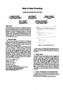
Fig. 4. Throughput of the two implementations using 192 cores, based on disk-based and memory-based cases with the four datasets.

calculated by dividing the input size (in plain format) by the algorithm runtime, and (b) statements processed per second that is calculated by dividing the number of processed statements by the runtime. From Table 4, our approach is 2.9 − 7.3× faster than the MapReduce-based approach for disk-based computation, and 2.6 − 7.4× for in-memory as illustrated in Table 5. The smallest speedup occurs for the BTC2011 benchmark, however it should be noted that in this instance, whereas we compress N-Quads, MapReduce discards the fourth term in the input data and just compresses the first three terms. Moreover, the compression throughput of Uniprot in both cases is much higher than the other three datasets. We attribute this to the large number of recurring popular terms and also the short length of terms, and thus the whole dataset can be processed quickly. For example, we can see that the average length of a term in Uniprot is smaller than other datasets from Table 2. In the meantime, we can calculate that each term in Uniprot appears about 17.8 times9 , which is higher than that of LUBM (12.6 times) and BTC2011 (16.3 times). Though this value in DBPedia is the greatest one (22.6 times), the processed time of this 9. The average time a term appears is calculated by where i = 3 for triples and i = 4 for N-Quads.

#stats.×i , #unique terms


TABLE 6 Processing 1M Statements in the Transactional Scenario # Stats per chunk

MapR.

100 1K 10K 100K

439 441 454 454

Avg. runtime per 10 chunks (sec.) X10 X10 Para. 0.211 0.359 1.761 17.177

8.1.3

TABLE 7 Incremental Update Scenario with different chunk size

# Chunks

Chunk Size

1 2 4 8

190 GB 95 GB 47 GB 23 GB

0.164 0.391 0.648 2.192

dataset is very small (less than 1 minutes), the overhead of the underlying implementation (message passing etc.) could start to impact the throughput. Comparing the two cases, the in-memory compression is faster than the disk-based one for both algorithms, although not dramatically so. Moreover, the improvements we achieved in Table 5 are greater than those in Table 4 for the LUBM and Uniprot data sets, marginally greater for DBpedia and slightly smaller for the BTC2011 data set. This illustrates that the two algorithms gain disproportionally from the faster I/O over different data sets (with our system showing better gains overall). Additionally, Figure 4 shows that the maximum number of statements processed per second we have achieved is about 6.51M, higher than any method in the literature. Transactional

We simulated two transactional processing scenarios with in-memory compression: (1) sequential transactions on a single node and (2) multiple parallel transactions on multiple nodes using the LUBM data set. To simulate transactions, we first encode the 1.1 billion triples in the LUBM8000 benchmark. Next, we prepare a RDF data set that contains 1M triples, split into 10K, 1K, 100, and 10 chunks, respectively. After encoding is complete, we encode these new input chunks (every 10 chunks) sequentially and record the corresponding encoding time. For the multiple parallel transaction scenario, we could only record the encoding time for our implementation since Hadoop uses a centralized model for data storage. Results are presented in Table 6. One can clearly observe that our approach is orders of magnitude faster than the MapReduce approach for the sequential case. The latter is neither optimized nor suitable for this use-case, since the startup overhead dominates the runtime, as evident from the observation that the average time to process chunks with different sizes is approximately the same. For our system, we observe that the average runtime of our approach increases with increasing chunk sizes, and the trend moves toward linear for the sequential case. This means that, for a single place, overhead takes a larger proportion of the runtime. Since we are using 192 cores and the number of chunks used in this scenario is 10, for each transaction with the parallel processing by our prototype, the chunks can be compressed at once by 10 places in parallel. The results in Table 6 show that the runtime is around 0.2 seconds when the number of statements is less than 100 in each chunk, which is slightly worse than our expectations for real-time applications, although still well within an acceptable range. Upon further analysis, we have found that this increase in

11

Runtime (sec.) MapR. X10 1739 2468 3900 6704

453 551 755 1164

Imprv. 3.8 4.5 5.2 5.8

program runtime is due to underlying bottlenecks in the X10 runtime implementation, which we have not addressed in this paper: (a) Every async call forks an underlying pthread (Posix thread) atomically, which leads to execution time overhead. (b) Type initializations in X10 are expensive, because all type initializations are internally guarded by locks. Our implementation still performs reasonably well even with these implementation overheads. 8.1.4

Updates

We evaluate the incremental updates scenario for RDF compression again using the LUBM8000 dataset and by splitting it into 2, 4, and 8 chunks, respectively. The resulting datasets are compressed in 2, 4 and 8 different executions respectively. Before each compression cycle, we empty the cache as to simulate real world conditions. The results comparing our approach and MapReduce are shown in Table 7. As expected, the performance for both algorithms decreases with increasing number of chunks, because of the additional process required during the encoding (e.g. reading the dictionary into memory). However, the increase in program runtime for our approach is much smaller than MapReduce. A possible explanation is that because our dictionary reading operation is faster, the startup overhead of our system is lower. It is also possible that the efficacy of the popularity caching technique used by MapReduce decreases disproportionately as the number of chunks increases. 8.2

Scalability

We test the scalability of our algorithm by varying the number of processing cores and the size of the input data set. We use the LUBM benchmark in our tests as it facilitates the generation of datasets of arbitrary size. 8.2.1

Number of Cores

We fix the input data set to 1.1 billion triples and double the number of cores from 12 (single node) till 384. The test results for our algorithm and the MapReduce-based approach are shown in Figure 5(a). These results demonstrate that the run time for both algorithms decreases with an increase in the number of cores. The speedup obtained with an increasing number of cores compared to a baseline of 12-cores for both algorithms is presented in Figure 5(b). In our system, with a small number of cores, the runtime is not linear, since for a single node there is no network communication. Nevertheless, starting from 24 cores, the speedup becomes almost linear (scaled speedup, not shown in the figure, is approximately 1.95). This result supports our theoretical analysis in Section 6.4, and we attribute the small amount of loss to network traffic. In contrast, the speedup of the

IEEE TRANSACTIONS ON PARALLEL AND DISTRIBUTED SYSTEMS, VOL. X, NO. X, 201X 1 8 0 0 0

1 6 8 8 9

M a p R . X 1 0

1 6 0 0 0 1 4 0 0 0

T im e ( s )

1 2 0 0 0 1 0 0 0 0 7 4 5 4

8 0 0 0 5 6 5 8

6 0 0 0

3 8 8 3

3 5 3 8

4 0 0 0

2 1 8 9

1 8 1 8

2 0 0 0

1 7 3 9 9 3 3

1 3 1 1 4 5 3

2 3 5

0 1 2

2 4

4 8

9 6

1 9 2

3 8 4

N u m b e r o f C o re s

(a) Runtime by varying nodes 2 5 M a p R . X 1 0 id e a l

2 0

S p e e d u p

1 5

1 0

5

0 0

5 0

1 0 0

1 5 0

2 0 0

2 5 0

3 0 0

3 5 0

4 0 0

N u m b e r o f C o re s

(b) Speedups by varying nodes 1 4 0 0 0 M a X 1 X 1 X 1

1 2 0 0 0

p R 0 _ 0 _ 0 _

. 1 5 1 0

1 0 0 0 0

T im e ( s )

8 0 0 0

12

We start our tests with 690 million triples and repeatedly double the size of the input until we reach a dataset comprising 11 billion triples. Additionally, for each dataset, we also vary the number of chunks read per loop for our implementation. The results are presented in Figure 5(c). We see that the runtime for both algorithms is nearly linear with the size of the input data sets. We also notice that MapReduce achieves a slightly super-linear speedup until 5.5 billion triples. After that, MapReduce speedup becomes linear with the input size. For our algorithm, we have experimented with 1, 5, and 10 chunks in each loop. One can see that the scalability of our algorithm is not linear with input data when reading 1 chunk per loop. But, speedup becomes better as we increase the number of chunks read per loop, and it matches the ideal linear speedup scenario when reading 10 chunks per loop. The reason may be the same as for the transactional case mentioned above, i.e. that a large number for loop results in additional runtime overheads as a result of forking threads and object type initializations. Small chunks also results in redundant filter and push operations for the same terms at the same place in different loops. Such an interpretation is in sympathy with our expectations described in Section 6.1. Furthermore, Figure 5(c) investigates the trade-off between reduced memory consumption and performance as well. For the optimal scalability case with reading 10 chunks at a time, we need to process 10 × 140K = 1.4M triples in each loop. Since, in Table 2, we show that 1.1 billion triples is about 190 GB, the size of 1.4 million triples would be about 250 MB, which is well within the RAM availability of most machines. Not withstanding this optimal case implementations using 5 chunks at a time (125 MB) and 1 chunk at a time (25 MB) is only accompanied with little and moderate scalability loss respectively.

6 0 0 0 4 0 0 0

8.3

2 0 0 0

We measure the load-balance characteristics of our algorithm in terms of five metrics defined later in this section. We instrument our code with counters to gather data for the first four metrics. The data for the final metric is obtained using the tracing option provided by the X10 implementation.

0 0

2

4

6

8

1 0

1 2

B illio n s o f T r ip le s

(c) Runtime by varying size Fig. 5. Scalability of two algorithms: (a) encoding 1.1 billion triples with varying the number of computation cores from 12 to 384, (b) the corresponding speedups achieved by varying the cores, and (c) the number of triples starts with 690 million and repeatedly double to 11 billion (192 cores, on disk)

MapReduce-based approach is almost linear (even superlinear) initially before plateauing for values of 92 cores and greater. This result mirrors the results obtained in [7]. There can be several reasons for the latter slowdown: we hypothesize that may be due to load imbalance, increased I/O traffic and platform overhead. 8.2.2 Size of Datasets To study the scalability of our algorithm with increasing input data size, we create a large LUBM data set with 11 billion triples, which is roughly equivalent to the LUBM80000 benchmark. We split this data set into a number of chunks, each of which contains 140K triples, allowing us to study the effect of loop from Algorithm 5.

Load Balancing

•

•

• • •

number of outgoing terms: The number of terms transferred to a remote place. This metric gives insight into the communication load balance achieved by our algorithm. For example, the larger the number of outgoing terms, the greater the associated network traffic. number of misses: The number of terms that are not already encoded (missed) in the dictionary and hence require the generation of a new id. miss ratio: The number of misses divided by the sum of hit and miss for the local dictionary. number of processed terms: the number of terms processed by a computing node. received bytes: the size of processed terms in bytes at a computing node.

We encoded 1.1 billion LUBM triples on a varying number of cores to gather data for the first three metrics described above. The results are presented in Table 8. We can see that the average values of the three metrics for all


TABLE 8 Term Information during encoding 1.1 billion triples

# Core 24 48 96 192 384

# Outgoing (M) Max Avg.

# Misses (M) Max Avg.

Miss Ratio Max Avg.

11.65 5.85 2.94 1.48 0.74

10.95 5.46 2.73 1.35 0.90

95.7% 96.1% 96.1% 96.4% 96.4%

11.59 5.78 2.89 1.43 0.70

10.95 5.46 2.73 1.35 0.87

94.5% 94.5% 94.5% 94.5% 94.5%

received is 1.37M in our approach, also showing minimal skew). Furthermore, when comparing the sum total of bytes received across the two implementations, it is clear that our proposed technique results in better performance, figures that confirm our theoretical analysis in Section 4.3. Consequently even when comparing with the reduce phase of MapReduce, our system results in a lighter workload and less network communication overhead.

9 TABLE 9 Comparison of Received Data for each computing node when processing 1.1 billion triples using 192 cores (In millions)

Algorithm Job1 Job2 Job3

MapR. X10

Recv. Bytes Max. Avg.

Recv. Records Max. Avg.

9.94 135.61 120.81

4.02 79.77 106.82

24.04 30.91 19.61

1.73 17.28 17.28

194.71

187.82

1.48

1.43

the tests are very close to the maximum values, suggesting excellent load balancing performance. The scalability of our algorithm with an increasing number of processing cores is highlighted well in these results. There is a clear linear decrease in all three metrics with an increase in the number of processing cores. Finally, the results also illustrate a consistent almost uniform miss probability for each dictionary. The average miss ratio is about 94.5%, indicating that we have redundant computation on average for 5 out of every 100 terms. This ratio approached the ideal value of 100%, which is nevertheless difficult to achieve in a distributed systems without significant coordination overhead. Additionally, our implementation is still based on the all-to-all communication, which could possibly effect the performance. However, our system does not repartition all the data, but only transfers the mappings that are necessary for each node. In this sense, our system performs useful computation in terms of data locality in 94.5% of the cases, meaning that although our approach does require communication between all nodes, only moving the data that actually needed. The last two metrics capture the load at each compute node in terms of the number of terms processed and size of data received in bytes. These metrics are important for measuring computational load balance and are used here to provide comparison with the performance available using the MapReduce approach. Since MapReduce divides the whole compression into three separate jobs and the implementation does not provide the relative metrics, we extract the reduce input records and reduce shuffle bytes in the reduce phase of each job from the Hadoop logs. These two items indicate the number of records processed and the corresponding data sizes for each of the 192 reduce tasks. The results are summarized in Table 9 and demonstrate that the difference between the maximum and the average value of these metrics for our implementation is much smaller than MapReduce, indicating better load balancing (in addition to the results, the minimum number of bytes received is 184.70M and the minimum number of records

13

C ONCLUSIONS

In this paper, we have summarized the challenges of distributed dictionary encoding of RDF data and discussed the possible performance issues of the current approaches through theoretical analysis. Based on that, we have introduced a new dictionary encoding algorithm for the fast compression of big Semantic Web data. We have described the detailed implementation of our algorithm utilising the X10 parallel programming language. We find that, using the X10, and in turn the APGAS model, has a number of advantages: (a) flexible and efficient scheduling. APGAS, like PGAS, separates tasks from underlying concurrency model, thereby allowing one to implement an efficient scheduling strategy irrespective of the number of tasks forked using async. (b) APGAS being derived from both MPI and OpenMP programming models, extracts parallelism at both the distributed and single machine hierarchies. (c) Finally, an abstract model provided by the async, finish, places, and activities, helps one write short code, which is easier to debug and maintain. We have presented an extensive quantitative evaluation of the proposed algorithm and conducted a comparison with a state-of-art approach using the MapReduce model [7]. The experimental results show that our proposed algorithm is: (a) Highly scalable both with increments in number of cores and in the size of the dataset, (b) Computationally fast, encoding 11 billion statements in about 1.2 hours, and achieving a 2.6 − 7.4× improvement over the MapReduce-based method, (c) Flexible for various semantic application scenarios, (d) Robust against data skew, showing excellent load balancing, and (e) Suitable for use and further development as part of a high performance distributed system. Actually, we have adopted the encoding algorithm in a large RDF analysis framework [38], [44] and the preliminary results show that the method can vastly improve data loading speeds for high throughput index building. We believe that our approach will also contribute to other semantic applications (e.g. reasoning [42]) in large-scale distributed scenarios.

ACKNOWLEDGMENTS Long Cheng is supported by the DFG in projects DIAMOND (Emmy Noether grant KR 4381/1-1) and HAEC (CRC 912). The computations were performed on the Highperformance Systems Research Cluster at IBM Research Ireland. The authors would like to thank the anonymous reviewers for their careful reading of the manuscript and many insightful comments and suggestions, which has great help for improving the work.


R EFERENCES [1] [2] [3]

[4] [5] [6]

[7] [8] [9] [10] [11] [12]

[13] [14] [15] [16] [17]

[18] [19] [20] [21] [22] [23]

[24] [25]

C. Bizer, T. Heath, and T. Berners-Lee, “Linked data - the story so far,” International Journal on Semantic Web and Information Systems, vol. 5, no. 3, pp. 1–22, 2009. S. Auer, C. Bizer, G. Kobilarov, J. Lehmann, R. Cyganiak, and Z. Ives, “DBpedia: a nucleus for a web of open data,” in Proc. 6th Int. Semantic Web Conf., 2007, pp. 722–735. R. Apweiler, A. Bairoch, C. H. Wu, W. C. Barker, B. Boeckmann, S. Ferro, E. Gasteiger, H. Huang, R. Lopez, M. Magrane, M. J. Martin, D. A. Natale, C. O’Donovan, N. Redaschi, and L.-S. L. Yeh, “Uniprot: the universal protein knowledgebase,” Nucleic Acids Research, vol. 32, pp. 115–119, 2004. ¨ C. Stadler, J. Lehmann, K. Hoffner, and S. Auer, “Linkedgeodata: A core for a web of spatial open data,” Semantic Web Journal, 2011. W3C, http://www.w3.org/RDF/. P. Charles, C. Grothoff, V. Saraswat, C. Donawa, A. Kielstra, K. Ebcioglu, C. Von Praun, and V. Sarkar, “X10: an object-oriented approach to non-uniform cluster computing,” ACM SIGPLAN Notices, vol. 40, no. 10, pp. 519–538, 2005. J. Urbani, J. Maassen, N. Drost, F. Seinstra, and H. Bal, “Scalable RDF data compression with MapReduce,” Concurrency and Computation: Practice and Experience, vol. 25, pp. 24–39, 2013. L. Cheng, A. Malik, S. Kotoulas, T. E. Ward, and G. Theodoropoulos, “Efficient parallel dictionary encoding for RDF data,” in Proc. 17th Int. Workshop on the Web and Databases, 2014. Z. Chen, J. Gehrke, and F. Korn, “Query optimization in compressed database systems,” in Proc. ACM SIGMOD Int. Conf. Management of Data, 2001, pp. 271–282. D. Abadi, S. Madden, and M. Ferreira, “Integrating compression and execution in column-oriented database systems,” in Proc. ACM SIGMOD Int. Conf. Management of Data, 2006, pp. 671–682. J. D. Fernández, C. Gutierrez, and M. A. Mart´ınez-Prieto, “RDF compression: basic approaches,” in Proc. 19th Int. Conf. World Wide Web, 2010, pp. 1091–1092. K. Lee, J. H. Son, G.-W. Kim, and M. H. Kim, “Web document compaction by compressing URI references in RDF and OWL data,” in Proc. 2nd Int. Conf. Ubiquitous Information Management and Communication, 2008, pp. 163–168. J. Weaver and G. T. Williams, “Reducing I/O load in parallel RDF systems via data compression,” in Proc. 1st Workshop on HighPerformance Computing for the Semantic Web, 2011. P. Yuan, P. Liu, B. Wu, H. Jin, W. Zhang, and L. Liu, “TripleBit: a fast and compact system for large scale RDF data,” Proc. VLDB Endowment, vol. 6, no. 7, pp. 517–528, 2013. H. R. Bazoobandi, S. de Rooij, J. Urbani, A. ten Teije, F. van Harmelen, and H. Bal, “A compact in-memory dictionary for RDF data,” in Proc. 12th European Semantic Web Conf., 2015, pp. 205–220. J. D. Fernández, M. A. Mart´ınez-Prieto, and C. Gutierrez, “Compact representation of large RDF data sets for publishing and exchange,” in Proc. 9th Int. Semantic Web Conf., 2010, pp. 193–208. J. M. Giménez-Garc´ıa, J. D. Fernández, and M. A. Mart´ınez-Prieto, “HDT-MR: A scalable solution for RDF compression with HDT and MapReduce,” in Proc. 12th European Semantic Web Conf., 2015, pp. 253–268. A. Owens, A. Seaborne, N. Gibbins, and mc schraefel, “Clustered TDB: A clustered triple store for Jena,” November 2008. J. Broekstra, A. Kampman, and F. van Harmelen, “Sesame: A generic architecture for storing and querying RDF and RDF schema,” in Proc. 1st Int. Semantic Web Conf., 2002, pp. 54–68. T. Neumann and G. Weikum, “RDF-3X: a risc-style engine for RDF,” Proc. VLDB Endowment, vol. 1, pp. 647–659, 2008. O. Erling and I. Mikhailov, “RDF Support in the Virtuoso DBMS,” in Networked Knowledge-Networked Media, 2009, pp. 7–24. M. Poess and D. Potapov, “Data compression in oracle,” in Proc. 29th Int. Conf. Very Large Data Bases, 2003, pp. 937–947. P. Boncz, T. Grust, M. van Keulen, S. Manegold, J. Rittinger, and J. Teubner, “MonetDB/XQuery: a fast XQuery processor powered by a relational engine,” in Proc. ACM SIGMOD Int. Conf. Management of Data, 2006, pp. 479–490. A. Harth, J. Umbrich, A. Hogan, and S. Decker, “YARS2: a federated repository for querying graph structured data from the web,” in Proc. 6th Int. Semantic Web Conf., 2007, pp. 211–224. J. Huang, D. J. Abadi, and K. Ren, “Scalable SPARQL querying of large RDF graphs,” Proc. VLDB Endowment, vol. 4, pp. 1123–1134, 2011.

14

[26] M. Feng, C. Lin, and R. Gupta, “PLDS: Partitioning linked data structures for parallelism,” ACM Trans. Archit. Code Optim., vol. 8, pp. 38:1–38:21, 2012. [27] E. L. Goodman, E. Jimenez, D. Mizell, S. al Saffar, B. Adolf, and D. Haglin, “High-performance computing applied to semantic databases,” in Proc. 8th European Semantic Web Conf., 2011, pp. 31– 45. [28] J. Dean and S. Ghemawat, “MapReduce: simplified data processing on large clusters,” Commun. ACM, vol. 51, no. 1, pp. 107–113, 2008. [29] Billion Triple Challenge, http://challenge.semanticweb.org. [30] W. Gropp, E. Lusk, N. Doss, and A. Skjellum, “A highperformance, portable implementation of the MPI message passing interface standard,” Parallel computing, vol. 22, no. 6, pp. 789– 828, 1996. [31] L. Dagum and R. Enon, “OpenMP: an industry standard API for shared-memory programming,” Computational Science & Engineering, IEEE, vol. 5, no. 1, pp. 46–55, 1998. [32] B. L. Chamberlain, D. Callahan, and H. P. Zima, “Parallel programmability and the Chapel language,” International Journal of High Performance Computing Applications, vol. 21, no. 3, pp. 291– 312, 2007. [33] T. El-Ghazawi and L. Smith, “UPC: unified parallel C,” in Proc. ACM/IEEE Conf. Supercomputing, 2006. [34] M. Zaharia, M. Chowdhury, T. Das, A. Dave, J. Ma, M. McCauley, M. J. Franklin, S. Shenker, and I. Stoica, “Resilient distributed datasets: A fault-tolerant abstraction for in-memory cluster computing,” in Proc. 9th USENIX Conf. Netw. Syst. Des. Implementation, 2012, pp. 15–28. [35] L. George, HBase: the definitive guide. ” O’Reilly Media, Inc.”, 2011. [36] A. Lakshman and P. Malik, “Cassandra: a decentralized structured storage system,” ACM SIGOPS Operating Systems Review, vol. 44, no. 2, pp. 35–40, 2010. [37] J. Zawodny, “Redis: Lightweight key/value store that goes the extra mile,” Linux Magazine, vol. 79, 2009. [38] L. Cheng, S. Kotoulas, T. Ward, and G. Theodoropoulos, “A fully parallel framework for analyzing RDF data,” in Proc. 13th Int. Semantic Web Conf., Posters & Demonstrations Track, 2014. [39] S. Kotoulas, E. Oren, and F. van Harmelen, “Mind the data skew: distributed inferencing by speeddating in elastic regions,” in Proc. 19th Int. Conf. World Wide Web, 2010, pp. 531–540. [40] R. W. Numrich and J. Reid, “Co-Array Fortran for parallel programming,” in ACM SIGPLAN Fortran Forum, vol. 17, no. 2, 1998, pp. 1–31. [41] J. Urbani, J. Maassen, and H. Bal, “Massive semantic web data compression with MapReduce,” in Proc. 19th ACM Int. Symp. High Performance Distributed Computing, 2010, pp. 795–802. [42] J. Urbani, S. Kotoulas, J. Maassen, F. Van Harmelen, and H. Bal, “WebPIE: A web-scale parallel inference engine using MapReduce,” Web Semantics: Science, Services and Agents on the World Wide Web, vol. 10, pp. 59–75, 2012. [43] Y. Guo, Z. Pan, and J. Heflin, “LUBM: A benchmark for OWL knowledge base systems,” Web Semantics: Science, Services and Agents on the World Wide Web, vol. 3, pp. 158 – 182, 2005. [44] L. Cheng, S. Kotoulas, T. Ward, and G. Theodoropoulos, “High throughput indexing for large-scale semantic web data,” in Proc. 30th Annual ACM Symp. Applied Computing, 2015, pp. 416–422.

Long Cheng is currently a Post-Doctoral Researcher at TU Dresden, Germany. His research interests mainly include distributed computing, large-scale data processing, data management, and Semantic Web. He was at organizations such as Huawei Technologies Germany and IBM Research Ireland. He holds a B.E. from Harbin Institute of Technology, China (2007), M.Sc from ¨ Duisburg-Essen, Germany (2010) Universitat and Ph.D from National University of Ireland Maynooth, Ireland (2014).


Avinash Malik is a Lecturer at the University of Auckland, New Zealand. His main research interest lies in programming languages for multicore and distributed systems and their formal semantics/compilation. He has worked at organizations such as INRIA in France, Trinity College Dublin, IBM Research Ireland and IBM Watson Research Centre on design and compilation of programming languages. He hold B.E. and PhD degrees from the University of Auckland.

Spyros Kotoulas is a Research Scientist at IBM Research Ireland. His research interests lie in data management for semi-structured data, parallel methods for data intensive processing, SemanticWeb, Linked Data, reasoning withWeb data, flexible data integration methods, stream processing, peer-to-peer and other distributed systems. He holds a BSc (2004) from the University of Crete as well as an MSc (2006) and a PhD (2009), both from the VU University Amsterdam.

Tomas E Ward is Senior Lecturer in Electronic Engineering at Maynooth University (since 1999) where he leads the Biomedical Engineering Research Group. Dr. Ward holds B.E. (Electronic Engineering), M.Eng.Sc. (Rehabilitation Engineering) and Ph.D (Biomedical Engineering) degrees from University College, Dublin. His academic research includes the application of neurotechnology for neurorehabilitation particularly in stroke and distributed signal processing stacks for connected health. Dr Ward has authored more than 200 peer-reviewed publications and has supervised to completion 20 research students (12 PhD). He has licensed a range of technologies to industry since 2009 including sensor streaming technologies for e-health, over the air programming and mobile health applications.

Georgios Theodoropoulos is the Executive Director of the Institute of Advanced Research Computing and holds a personal chair in the School of Engineering and Computing Sciences at Durham University in the UK. He joined Durham from IBM Research Lab in Dublin where as a Senior Research Scientist he helped establish the Lab’s Exascale Systems research programme. His research interests and contributions are in the areas of High Performance Computing Systems, Big Data; Complex and Multi-agent systems; Modelling and Distributed Simulation; large scale distributed infrastructures and Prescriptive Analytics for complex sociotechnical systems.

15