Fast Computation Kenneth Columbia
of Sparse Datacubes
A. ROSS*
Divesh
University
AT&T
karQcs.columbia.edu
[email protected]
1 Abstract Datacube queries compute aggregates over database relations at a variety of granularities, and they constitute an important class of decision support queries. Real-world data is frequently sparse, and hence efficiently computing datacubes over large sparse relations is important. We show that current techniques for computing datacubes over sparse relations do not scale well with the number of CUBE BY attributes, especially when the relation is much larger than main memory. We propose a novel algorithm for the fast computation of datacubes over sparse relations, and demonstrate the efficiency of our algorithm using synthetic, benchmark and real-world data sets. When the relation fits in memory, our technique performs multiple in-memory sorts, and does not incur any I/O beyond the input of the relation and the output of the datacube itself. When the relation does not fit in memory, a divideand-conquer strategy divides the problem of computing the datacube into several simpler computations of sub-datacubes. Often, all but one of the sub-datacubes can be computed in memory and our in-memory solution applies. In that case, the total I/O overhead is linear in the number of CUBE BY attributes. We demonstrate with an implementation that the CPU cost of our algorithm is dominated by the I/O cost for sparse relations. ‘The research of Kenneth A. Ross was supported by a grant from the AT&T Foundation, by a David and Lucile Packard Foundation Fellowship in Science and Engineering, by a Sloan Foundation Fellowship, by an NSF Young Investigator Award, and by NSF CISE award CDA-9625374. Permission to copy without fee 011 or port of this material is gmnted provided that the copies ore not made or distributed for direct commercial advantage, the VLDB copyright notice and the title of the publication and its dote appear, and notice is given that copying is by permission of the Very Large Data Bose Endowment. To copy otherwise, or to republish, requires a fee and/or special permission from the Endowment. Proceedings of the 23rd Athens, Greece, 1997
VLDB
Conference
Srivastava Labs-Research
Introduction
Datacube queries compute aggregates over relations at a variety of granularities, and they constitute an important class of decision support queries. The databases may represent business data (such as point-of-sales transactions), medical data (such as patient treatments and outcomes), or scientific data (such as large sets of experimental measurements). An example datacube query is “Broken down by supplier, part and month, find the total sales in 1996, including all subtotals across each dimension.” The attributes constituting the dimensions along which the aggregates are computed are called CUBE BY attributes. In the query above, for example, the CUBE BY attributes are supplier, part and month. A relation is sparse with respect to a set of attributes if its cardinality is a small fraction of the size of the crossproduct of the attribute domains. We are particularly interested in relations that are sparse with respect to the CUBE BY attributes for a given datacube query; when the attributes are understood from the context we will simply refer to the relation as sparse. Sparseness exists for two distinct reasons: large domain and a large number of sizes of some CUBE BY attributes CUBE BY attributes in the datacube query. Real-world data in application domains is often very large and sparse. Hence, efficiently computing datacubes over large sparse relations is important. The contributions of this paper are described below. We show that current techniques for computing datacubes are not very efficient for sparse relations, especially when the database relation is much larger than main memory (Section 2). We propose a novel algorithm, Partitioned-Cube, for the fast computation of datacubes over large sparse relations (Section 3). Partitioned-Cube uses a divide-andconquer strategy that divides the problem of computing the datacube over a relation with T tuples and k CUBE BY attributes into n + 1 sub-datacubes, for a large number n. The first n of these sub-datacubes each has approximately T/n tuples and k CUBE BY attributes. The final sub-datacube has no more than T tuples and has k - 1 CUBE BY attributes. We formulate an algorithm, Memory-Cube, for the efficient computation of datacubes over relations that fit in memory (Section 4). Memory-Cube performs multiple in-
116
Figure
1: Datacube
Query
Q
memory sorts, and does not incur any I/O beyond the input of the relation and the output of the datacube itself. Memory-Cube performs as few sorts as possible, and it takes advantage of common prefixes between multiple sort orders to optimize the CPU cost. cost of the analyze then We I/O Algorithm Partitioned-Cube (Section 5). Often each of the first n sub-datacubes of Algorithm Partitioned-Cube can be computed in memory using Memory-Cube. In that case, the total I/O cost of our algorithm is linear in the number of CUBE BY attributes, unlike previous techniques for computing datacubes. We demonstrate the efficiency of our algorithms using synthetic, benchmark and real-world data sets, and show with an implementation that the CPU cost of our algorithm is dominated by the I/O cost for sparse relations, often by an order of magnitude (Section 6). To our knowledge, ours is the first work specifically addressing datacube computations for the important class of sparse database relations.
2
Motivation:
Existing
Q(gj) can be computed using cuboid Q(&) if and only if Zj is of coarser granularity than &. The various existing techniques for computing datacubes, outlined below, attempt to make use of the relationships between the cuboids to compute the datacube Q more efficiently than the naive approach of independently computing each of the 2k cuboids.
Techniques
We present the ideas that underlie various existing techniques for computing datacubes using the datacube query Q in Figure 1, expressed in the generalized SQL syntax of Gray et al. [GBLPSG]. Here A and the Bi’s are attributes of the relation R, and G is an aggregate function. In this paper, we consider only distributive aggregate functions [GBLP96]. The computation of Q involves the computation of aggregates over the relation R at 2k different granularities, where each granularity is one of the 2” possible subsets of the CUBE BY attributes Br, . . . , Bk; attributes that are not present in such a subset are replaced by a special value “ALL” in the datacube result. Each of these 2’ granularities is referred to as a cuboid following [DANR96, AAD+96], and we use the notation Q(&) to denote the cuboid at granularity &. The computation of the various cuboids are not independent of each other, but are closely related in that some of them can be computed using others. These relationships are captured in terms of the search lattice for the datacube (HRU96J. Each granularity & C @I , . . . , Bk) is a node in the search lattice, and there is an edge from node & to B” if ?ij is a subset of and has one fewer element than &; $ is said to be a parent of gj in the search lattice. If there is a path from 5; to B’j in the search lattice, & is said to be of a finer granularity than gj, and Bj is said to be of a coarser granularity than gi. Paths in the search lattice precisely determine which of the cuboids can be computed from which others. In particular, cuboid
2.1
PIPESORT
The PLPESORT algorithm proposed by Sarawagi et al. [SAG96, AAD+ tries to optimize the overall cost of the computation of datacube Q using cost estimates of various ways to compute each cuboid Q(gj) to determine which cuboid will be used to actually compute the tuples of Q(gj). First, PIPESORT annotates each edge (&,gj) of the search lattice of datacube Q with two costs: S(&, gj) is the cost of computing Q&) from an unsorted Q(&), and A(&,Sj) is the cost of computing Q(gj) from a sorted Q(&>. Second, PIPESORT proceeds level-by-level in the search lattice, starting from the root, ordering the attributes at each node and prnning edges to convert the search lattice into a tree. If the attribute order of node gj is a prefix of the order of its parent node & in the tree, then Q(gj) can be computed from Q(&) without sorting, and the edge (&,gj) in the tree is marked A and has cost A(&,Zj). Otherwise, Q(&) has to be sorted to compute Q&j,, and edge (&,Zj) is marked S and has cost S(&, Zj). The marking is constrained by the requirement that at most one edge out of any node gi can be marked A. PIPESORT guarantees this using a local optimization technique based on weighted bipartite matching, that also minimizes the sum of edge costs at each level of the search lattice. Third, PIPESORT adds a node corresponding to the relation R to the tree, and adds an edge marked S from R to the root of the tree. PIPESORT then converts the resulting tree into a set of paths such that every edge in the tree is present in one and only one path, and all the edges in each path except the first edge are marked A. At evaluation time, the various paths are evaluated in turn. During the evaluation of a path with root & (or R), the tuples of Q(&) (or R) are sorted in the order indicated by the attribute ordering of the child $ of the root in the path. Once the tuples are sorted, the pipelined evaluation of the path requires only a single tuple to be maintained per non-root node in the path, which is very space efficient. The main limitation of PIPESORT is that it does not scale well with respect to the number of CUBE BY attributes in the datacube query. PIPESORT performs one sort operation for the pipelined evaluation of each path. When the number of CUBE BY attributes in Q is k, a lower bound on the number of such sorts performed by PIPESORT is given by ( Tkk/z,), which is exponential in Ic (see Section 4.1). When the underlying relation is sparse and much larger than available memory, then many of the cuboids that PIPESORT sorts are also larger than the available memory (see Section 5.1). Sorting these cuboids requires external
117
sorts, resulting in PIPESORT performing a considerable amount of I/O. The following example illustrates this problem with PIPESORT.
other cuboids, only a single page of memory can be allocated - these cuboids are said to be in the “SortRun” state. OVERLAP does the allocation using a heuristic of traversing the search tree in a breadth-first order, giving priority to cuboids with smaller partition sizes, and cuboids with longer attribute lists. Cuboids that are not chosen are considered in subsequent passes using the above steps to allocate memory and mark cuboids. At evaluation time, each set of cuboids that can be computed concurrently is evaluated in turn. Tuples of cuboids marked to be in the “Partition” state are immediately available for pipelining purposes. Tuples of cuboids marked to be in the “SortRun” state are simply written to disk; the various runs are subsequently merged, further aggregating as necessary, and the result tuples are pipelined for further computation. Since the amount of I/O performed by OVERLAP depends on the partition sizes and the number of sorted runs that have to be written to disk, the analysis of the I/O cost of OVERLAP is quite complicated. We provide an approximate lower bound below. When the underlying relation is sparse, many of the cuboids are no smaller than the relation (see Section 5.1). If the relation is large and does not fit in memory, then neither do these cuboids. There are O(L) nodes in the search tree of OVERLAP for which the partition sizes are the sizes of the corresponding cuboids. Further, the processing of each such node takes I/O which is the equivalent of five passes through the relation (one pass for writing out the tuples while processing the parent node, three passes for the external sort, and one pass for reading in the tuples of the node to process its children); this does not include the I/O cost of writing out the datacube result. Even when the cuboids are in the “Partition” state, and each partition fits in memory, the memory may not be large enough to accommodate more than one such partition at a time. (Example 2.1 is such an example.) Since each of these O(lc) nodes has O(k) such descendants (with the length of the maximum common prefix being l), there are at least O(k2) nodes in the search tree that involve additional I/O. This demonstrates that the I/O cost of OVERLAP is at least quadratic in k for sparse data sets, even assuming that partitioning R always gives memory-sized partitions!
Example 2.1 Consider a synthetic relation RI with 8 attributes, 7 of which are used as CUBE BY attributes and the eighth attribute is aggregated, to compute a datacube Qr over the relation RI. Suppose that the value of each CUBE BY attribute is uniformly distributed in the range 1 to 100, and the relation RI has 2 x 10s tuples. Since the 7 CUBE BY attributes together can range over a possible 1014 tuples, RI is a sparse relation. The datacube Qi in this case has a little over 9 x 10’ tuples, which makes it about 45 times bigger than the underlying relation RI. Assume that we have a 96MB main memory capable of holding 2.4 x 10’ values (this would correspond to 4-byte integer values). PIPESORT would perform at least (i) = 35 sorts over various intermediate datacube results, each of which is about the same size as the underlying relation RI and hence are much larger than main memory. Counting three passes per external sort, PIPESORT requires at least I/O equivalent to 3 * 35 = 105 passes through the relation. PIPESORT thus has an I/O overhead of more than 200% over the cost of writing out the datacube result, on this example. On this example, as we show later, the I/O overhead of our technique, Partitioned-Cube, is about the equivalent of 11.5 passes through the relation. It thus incurs an I/O overhead of only about 25%! (We shall address the CPU cost separately.) 0
2.2
OVERLAP
The OVERLAP algorithm proposed by Deshpande et al. [DANR96, AAD+96] tries to minimize the number of disk accesses by overlapping the computation of the cuboids, by making use of partially matching sort orders to reduce the number of sorting steps performed. First, OVERLAP computes the finest granularity cuboid Q({B~, . . . , Bk}) from R, and sorts the tuples of this cuboid in some order, say (Bi, . . . ,Bk). The attributes at each node of the search lattice are then ordered to be subsequences of this sort order. Second, OVERLAP prunes edges in the search lattice, converting it into a tree, as follows. Among the various parents of node gj in the search lattice, the parent of & in the tree is a node & that shares the longest prefix in the attribute ordering with gj. Third, nodes in the tree are labeled with estimates of the memory required to compute the corresponding cuboid from its parent, assuming that the tuples of the parent cuboid are sorted in the order indicated by the attribute ordering of the parent node. For example, if the attribute ordering of gj is a prefix of the attribute ordering of &, the estimate associated with Gj is 1 tuple, since the sort orders match. Fourth, a set of cuboids is chosen that can be computed concurrently within the available memory constraints. For some cuboids, the estimated memory can be allocated such cuboids are said to be in the “Partition” state. For
Example 2.2 Consider the datacube in Example 2.1. Using our approximate lower bound calculations, the I/O cost of OVERLAP is at least the equivalent of 21 passes through the relation. Assume that the sort order on the CUBE BY atThe tributes, chosen by OVERLAP, is (Br,. . . ,B7). I/O cost includes the equivalent of 5 passes through the database relation for each of the three cuboids Q({B~, . . ,B7}), . . , Q({B~, . . . ,Br}) that are the same size as the underlying relation, the equivalent of 2.5 passes through the relation for the cuboid Q((B4,. . . , B7)) that is half the size of the relation, and the equivalent of 2 passes for each of the two nodes that share a prefix of length one with ({Br , . . , Br}) and have to be in the SortRun state;
118
Algorithm INPUTS:
Partitioned-Cube@, {Bi, . . ,Bm}, A, G) A set of tuples R, possibly stored ,in horizontal fragments; CUBE BY attributes {Bi, . . . ,Bm}; attribute A to be aggregated; aggregate function G(.). The datacube result for R over {Bi, . . . , Bm} in two horizontal fragments F and D on disk. F OUTPUTS: contains the finest granularity datacube tuples (i.e., grouping by all of {Bi, . . . , Bm}), and D contains the remaining tuples. (F and D may themselves be further horizontally partitioned.) if (R fits in memory) then return Memory-Cube(R, {Bi, . . . , Bm}, A, G); METHOD: else { choose an attribute Bj among {Bi, . . . , B,}; scan R and partition on Bj into sets of tuples Ri, . . . , Rn; /* n 5 card(Bj) and n 5 number of buffers in memory */ for i = 1 . . . n let (F;,Di) = Partitioned-Cube&, {Bi,. . . ,B,,,},A, G); let F = the union of the Fi’s; let (F’,D’) = Partitioned-Cube(F, {Bi, . . . , Bj-1 ,Bj+i, . . . , B,,,}, A, G); let D = the union of F’, D’ and the D;‘s; return (F,D); } Figure
2: Algorithm
Part it ioned-Cube & (of Figure l), the algorithm is initially invoked as Partitioned-Cube(R, {Br, . . . ,Bk}, A, C). Algorithm Partitioned-Cube assumes the existence of a subroutine Memory-Cube that computes the datacube of a relation that fits in memory. We shall present Algorithm Memory-Cube in Section 4. Observe that Algorithm Memory-Cube must not need significant additional space beyond its input since the test for applicability of Algorithm Memory-Cube is simply whether the input relation fits in memory. The structure of Algorithm Partitioned-Cube follows the recursive structure of datacubes themselves. A datacube is obtained by fixing each possible value of a CUBE BY attribute Bj in turn and computing the tuples in the corresponding sub-datacube, followed by computing the datscube tuples with the value ALL for Bj. Rather than rereading the input relation R for the ALL datacube we read the finest granularity cuboid F, which may be significantly smaller than R if there are many tuples in each group, and is never larger than R. These observations form the basis of an inductive proof of the correctness of Algorithm Partitioned-Cube. An interesting feature of this algorithm is that the datacube of R is broken up into n + 1 smaller sub-datacube computations, n of which are likely to be much smaller than the original datacube, if the domain of the partitioning attribute Bj is sufficiently large. If there are T tuples in R, then we would expect roughly T/n tuples in each of the n partitions (in the absence of significant skew). Thus, it is relatively likely that, even for a relation significantly bigger than main memory, each of these n sub-datacubes can be computed in memory using Algorithm Memory-Cube. The n + l’st sub-datacube has one fewer CUBE BY attribute and no more than T tuples. Thus, the I/O cost will typically be proportional to the number of CUBE BY attributes k, and not exponential in k as PIPESORT or quadratic in k as OVERLAP.
one pass for writing the sorted runs and one pass for reading them in for subsequent processing. This analysis gives OVERLAP an I/O overhead of at least 45% over the size of the datacube result! 0
2.3
Array-Based
Algorithms
The array-based algorithm proposed by Gray et al. [GBLPW] is essentially a main memory algorithm, where all the tuples of the datacube are kept in memory as a k-dimensional array, where k is the number of CUBE BY attributes. The data structures needed by Gray et al’s algorithm will often not fit into memory for sparse relations, even when R does. In this case, the algorithm does QOt apply. The array-based algorithm proposed by Zhao et al. [ZDN97] overcomes some of the limitations of Gray et al.‘s algorithm. The data is partitioned and processed in an order that requires only fragments of the array to be present in memory at any one time. Data compression is also used to speed up the I/O. The algorithm of [ZDN97] performs particularly well because the array representation allows direct access to the needed cells. In the present paper we consider real-world data sets where the data is orders of magnitude more sparse than the synthetic data sets considered in [ZDNS’I]. For extremely sparse data, the array representation of [ZDN97] cannot fit into memory, and so a more costly data structure would be necessary.
3
Algorithm
Part it ioned-Cube
Our solution for the fast computation of the datacube is based on two fundamental ideas that have been successfully used for performing complex operations (such as sorting and joins) over very large relations: (a) partition the large relations into fragments that fit in memory, and (b) perform the complex operation over each memory-sized fragment independently. Our solution for computing a datacube query is a To compute recursive one, described in Figure 2.
Example 3.1 Figure 3 depicts the nodes in the search lattice of a datacube query with four CUBE BY attributes
119
4
R (Partitioned
Figure
Memory-Cube
Consider the case when the entire relation B fits in memory. We describe an efficient Algorithm Memory-Cube for computing the entire datacube. This technique is a critical building block in computing the cube using Algorithm Partitioned-Cube when the relation is much larger than memory. A crucial feature of this algorithm is that it computes the complete datacube without caching any of the datacube results for later reuse. Thus only a small amount of additional storage beyond the input relation is required.
by A)
3: An Illustrative
Algorithm
Example
{A,B, C, D}, and illustrates the order in which Algorithm Partitioned-Cube computes the various cuboids of the datacube, when the result of each partition fits into memory. The dashed arrows indicate that in-memory sorting (of the source node) takes place; the solid arrows indicate the computation of aggregates along paths with a common prefix. Assume that the order in which the attributes are chosen for partitioning purposes is (A, B, C, D). First, the underlying relation is partitioned by attribute A. Since each partition fits into memory, the partitions are fetched into memory one-at-at-time. When a partition is in memory, some tuples can be computed for each of the cuboids that have A as an attribute. When all the partitions have been processed, all tuples have been computed for these cuboids; in particular, all the tuples of cuboid Q({A, B, C, D}) have been computed. Next, the finest granularity cuboid Q({A, B, C, D}) is partitioned by attribute B. (Attribute A can be projected out during this phase.) The partitions are processed as before, and when all these partitions have been processed, all tuples have been computed for the cuboids that have attribute B (but not attribute A). Finally, the cuboid Q({B,C,D}) is determined to fit in memory. Hence, all the other cuboids can be computed without any further partitioning. 0 Algorithm Partitioned-Cube is adaptive to skew in the sense that partitions that fit in memory will be handled by Algorithm Memory-Cube, while larger partitions will be repartitioned. Repartitioning all partitions until the largest fits in memory is not performed. Algorithm Partitioned-Cube does not specify exactly how to partition, or how many partitions to create. Given a partitioning attribute Bj, the number n of partitions is bounded above by both the cardinality of the domain of Bj , and the number of buffers that can be allocated in memory. If n is less than the cardinality of the domain, then hashpartitioning or range-partitioning could be used. An optimization of Algorithm Partitioned-Cube would be to unfold multiple recursive calls if it is estimated in advance that several levels of partitioning will be necessary. If there is enough main memory to hold buffers for all of the partitions, a multi-dimensional partition can be obtained in one I/O scan.
Essentially, Memory-Cube computes the various cuboids of the datacube using the idea of pipelined paths of PIPESORT, where each path requires the relation to be sorted in a particular attribute ordering. The PIPESORT heuristic, however, does not guarantee that the number of paths used (and hence the number of sorts performed) is minimal. Hence, we first present an algorithm that determines an optimal set of paths (and hence the optimal number of sorts) that are needed to compute each cuboid in the datacube. We then show that the set of sorts that need to be performed are not independent of each other, but can share a considerable amount of computation. The combination of these two ideas provides a CPU efficient solution to the problem of computing the entire datacube when the relation fits in memory. Further, Memory-Cube does not incur any I/O beyond the input of the relation and the output of the datacube itself.
4.1
Paths
in the
Search
Lattice
Recall that paths in the search lattice determine which of the 2” cuboids can be computed from which others, and the evaluation of each path (as in PIPESORT) requires a sorting of the relation at the root node of the path. To minimize the number of (expensive) sort operations performed, it is hence desirable to minimize the total number of paths in the search lattice that are generated to cover all the nodes. However, the heuristic approach adopted in PIPESORT does not guarantee the optimality of this number of paths. There must exist at least ( lkTz,) paths, since the search lattice has that many nodes with [k/2] attributes, and no path in the search lattice can pass through two nodes with the same number of attributes. We now demonstrate that (,&) is also an upper-bound on the number of paths required to cover all the nodes in the search lattice, and we present a constructive procedure that achieves this bound. Our construction is a recursive procedure, described in Figure 4 as Algorithm Paths. The desired set of paths for the datacube query is given by Paths({Bi, . . . ,Bk}).
Example 4.1 Let the datacube query have CUBE BY attributes {A,B,C,D}. G(0) is given by E. We show G(1) through G(4). (Separate paths are shown on separate lines.)
120
Algorithm Paths({Bi, . . . , Bj}) CUBE BY attributes {Bi, . . . , Bj}. INPUTS: A set G(j) of (TjjZ,) paths in the search lattice that cover all the nodes. OUTPUTS: if (j = 0) then return a single node with an empty attribute list, c; METHOD: else { let G(j - 1) = Paths({Bi,. . . ,Bj-I}); let Gl(j - 1) and G,(j - 1) denote two replicas of G(j - 1); prefix the attribute list of each node of Gl(j - 1) with Bj; for each path Ni --t . . . + Np in G,(j - 1) { remove node Np and the edge into Np (if any) from G,(j - 1); add node Nr, to GI(J’ - 1); add an edge from node Bj . Np to node Np in Gl(j - 1); } return the union of the resulting Gl(j - 1) and G,(j - 1); } Figure G(1) G(2)
=
G(3)
=
G(4)
=
=
4: Computing
Paths for In-Memory
D+ E C.D+C--Ne D B.C.D+B.C+B+e B.D+D C.D+C A.B.C.D--tA.B.C--,A.B~A--,~ A.B.DhA.D+D A.C.D+A.C+C B.C.D-+B.C+B B.D C.D
4.2
Sharing
Sort Work
When computing the datacube from an in-memory relation, the relation in memory has to be sorted multiple times. The order in which this sequence of sorts is performed does not affect the correctness of the algorithm but could affect its performance. Consider Example 4.1. The relation needs to be sorted 6 times, in the following (named) orders: Si = A . B . C . D,
S2=~.~.~,S3=c.~.~,S4=~.c.~,ss=B.Dandss= C D. If the sequence in which the sorts are performed is S3, Ss , S3, S3 , S4, Si , then some computation that has been
Computation
performed in one sort can be utilized in the following sort. For example, Ss has sorted the relation in the attribute ordering C . D. To sort according to S3 now, the entire relation does not have to be resorted; only each block of tuples that share a C value needs to be independently sorted in the A.D order. Once this is done, the result will be sorted In Section 6 we demonstrate in the desired S3 order. experimentally that this sharing of sort order information has a significant positive impact on the running time.
4.3
Computing
the Cube by Traversing
Paths
Algorithm Memory-Cube, described in Figure 5, computes the datacube as follows: It takes a prefix-ordered path, and sorts the in-memory relation according to the attribute ordering of the initial node of the path. Like PIPESORT, it then makes a single scan through the data, accumulating along the way aggregates at all granularities on the path. Aggregates from finer granularities are combined with those at coarser granularities when the corresponding grouping attributes change. Datacube results are output immediately. The sort orders used by Memory-Cube are generated as described in Section 4.1, and processed in lexicographic order so that some of the sorting work can be shared as described in Section 4.2. There are (rk’f2,) sorting steps since there are that many paths.
The attributes of the paths in G(4) are finally reordered to obey the prefix property. G(4) has 6 paths, which is the desired number, i.e., (l); these paths completely cover the search lattice. Evaluating the datacube with 4 CUBE BY attributes, when the entire relation fits in memory, hence requires 6 in-memory sorts of the relation. These 6 sorting orders are obtained from the roots of the 6 paths in the prefix-sorted versionofG(4), as follows: A.B.C.D,D.A.B,C.A.D,B.C.D, B.D and C.D. Once the relation is sorted in the order determined by the root of a path, all the cuboids corresponding to the nodes in the path can be computed in a single pass over the relation. 0 It is easy to see that the algorithm generates paths that cover all the nodes of the search lattice. The proof that the algorithm generates precisely (,&,) paths is based on the symmetry of the algorithm. Details will appear in the full version of the paper.
Datacube
5
Analysis
of Our Solution
We analyze our solution for computing the datacube when all partitions of the data fit in memory.
5.1
Estimating
the Size of a Datacube
We now present analytical formulas estimating the number of tuples in each cuboid of, and in the result of, a datacube. Details will be presented in the full version of this paper. Let T be the number of tuples in the relation R, and assume that the value of each CUBEBY attribute of a tuple in B is randomly and independently drawn from the domain of that attribute. Let the cardinalities of the domains of Q’s k CUBEBY attributes, Bi,. . . ,Bk, be
121
Algorithm INPUTS:
Memory-Cube&l, {Bi, . ,B,,,}, A, G) A set of tuples B, that fits in memory; CUBE BY attributes {Br , . , B,,,}; attribute A to be aggregated; aggregate function G(.). OUTPUTS: The datacube result for B over {Br , , Bm} in two horizontal fragments F and D on disk. F contains the finest granularity datacube tuples (i.e., grouping by all of {Br, . . ,Bm}), and D contains the remaining tuples. sort R and combine all tuples that share all values of {Br , . . , B,}; METHOD: /* Assume that tuples are sorted according to first sort order */ for each sort order { initialize accumulators for computing aggregates at each granularity; combine first tuple into finest granularity accumulator; for each subsequent tuple t { compare t with previous tuple, to find the position j of the first sort order attribute at which they differ; if (j is greater than the number of common attributes between this sort order and the next) then { re-sort the segment from the previous tuple t’ at which this condition was satisfied up to the tuple prior to t according to the next sort order; } if (grouping attributes oft differ from those in finest granularity accumulator) then { output and then combine each accumulator into coarser granularity accumulator, until the grouping attributes of accumulator match with those oft; /* the number of combinings depends on the sort order length and on j */ 1 combine current tuple with the finest granularity accumulator; } } Figure
5: Algorithm
Memory-Cube
given by card(l), . . , card(k), respectively. Then the number of tuples in the cuboid Q({Bj,, . ,Bj,}) is given by cuboidsize( {jl , . , ji}, T), where: cuboidsize({jl,.
. , ji},T)
= shoot(T,ticard(jl))
l=l shoot(a,s) = s *
(1-
(1-
f)Q)
The total number of tuples in the datacube Q is given by cabesite(k, T), and is obtained by adding up the tuples in all the cuboids of Q. When the domains of ea>h of the CUBE BY attributes have the same cardinality, say card, cubesize(k, T) simplifies to: cubesize(k,T)
=
2
( (1‘)
* shoot(T, card’)
i=O Figure 6 shows the estimated ratio of the size of the datacube to the size of the input relation as a function of k, for various values of the (uniform) domain cardinality. The input relation has cardinality 106. Note the logarithmic vertical scale. 5.2
The
I/O
Cost
of Partitioned-Cube
Using our formulas for the cuboid size estimates, one can construct a cost-formula for Algorithm Partitioned-Cube. For cuboids that fit into memory, we count a single pass. For cuboids that don’t fit in memory, we count a read and write pass for partitioning, followed by a read pass to compute the sub-datacubes in each partition, assuming the partitions fit into memory. Under this assumption, it
Figure
6: Cube to Input
size ratio as a function
of k.
turns out that the total I/O cost is O(k 1R I). The details will appear in the full version of the paper. Example 5.1 Consider Example 2.1 once more. Algorithm Partitioned-Cube requires the processing of three cuboids (of dimensions 7, 6, and 5) whose inputs have size comparable to the original relation, one cuboid (of dimension 4) with input size comparable to half that of the original relation, and one cuboid (of dimension 3) of negligible input size. The total I/O overhead is thus roughly the equivalent of 11.5 passes through the relation. This is an overhead of only about 25% over the cost of writing the datacube result! 0 In contrast to Partitioned-Cube, the I/O cost of PIPESORT is exponential in k and the I/O cost of OVERLAP is quadratic in k, for sparse data sets, even under
122
the assumption that partitioning It always gives memorysized fragments. Ours is the only solution for computing the datacube that we are aware of, whose I/O cost in this scenario is linear in k, which makes our solution scalable! 5.3
The
CPU
Cost
The number of in-memory sorts needed is exponential in k. This exponential factor is unavoidable, because the width of the search lattice of the datacube is exponential in k. It remains to be seen whether or not the exponential CPU time dominates the I/O time in practice. We answer this question quantitatively in Section 6. As long as the total CPU time required to compute the datacube is less than the total I/O time needed to write the output result, we can use standard double-buffering techniques to decouple the CPU and I/O in order to run at the I/O bandwidth. In the full version of the paper we argue that the CPU cost of our algorithms is likely to be less than the CPU costs of PIPESORT and OVERLAP.
6
Experimental
Evaluation
We have implemented Algorithm Memory-Cube from Figure 5 in C++, and it computes the datacube of a partition that fits in memory. The data is read in, or is synthetically generated internally. Data is assumed to consist of 4-byte integer values on all grouping and aggregated attributes, and it is assumed that no extraneous attributes are present. The “combine” operation is a procedure that can be written to perform arbitrary incremental aggregate operators. In this section, we report results for a SUB operation over one attribute, and in one example a MAXoperation over one attribute. We ran the datacube algorithm on an UltraSparc singleprocessor model 170 with 96MB of RAM. The algorithm was run late at night when no other processes were active. We measured both the CPU time and the elapsed time. In all experiments reported, the CPU time and elapsed time were within one percent; in our results we use the CPU time. The time was measured from the point after the input relation was read or generated until the end of the datacube computation. We suppressed the I/O for the datacube output so that we could get an accurate measure of the CPU cost of computing the datacube. We observed that there was almost no page faulting activity during the running of the datacube code -thus there was no overhead due to thrashing. We did not try to measure I/O cost since we did not use a raw file system, and would have been likely to encounter substantial file-system overheads. Since the datacube output and relation input can be performed sequentially in a buffered fashion, we believe that an accurate approximation of the I/O time that would be expected in a commercial database system can be obtained by dividing the number of bytes to be read/written by the sustained sequential transfer rate of the disk drive being used. In the graphs below we assume a disk transfer rate of 1.5 MB/set, as in [SAG96, AAD+96].
Sorting was performed in-place (on pointers to tuples) using quicksort [Hoa62]. We ran several experiments with the following aims in mind: (a) To demonstrate that the algorithm is practical, and performs reasonably fast. (b) To assess the relative contributions of CPU time and I/O time for various data sets. (c) To measure properties of the algorithm, such as the benefit of sharing sort-orders compared with full resorting. (d) To verify that the algorithm scales appropriately. Example 6.1 In this example we consider data sets of size 104, 105, and lo6 tuples, with attribute values distributed uniformly within a common range. The range cardinalities were varied from 16 to 4096, and the number of CUBE BY attributes was varied from 1 to 9. With 9 CUBE BY attributes (and one aggregated attribute) the size of the largest relation considered was lo6 * 10 * 4 bytes, i.e., 40MB. Performance graphs are given in Figure 7. Graphs (a), (b) and (c) show the CPU time as a function of the number of tuples, for various numbers of CUBE BY attributes. (Note the logarithmic scale on both axes.) Graph (a) corresponds to a domain cardinality of 16, graph (b) to 64, and graph (c) to 1024. First, observe that in Figure 7(c) the graphs for 3, 5, 7 and 9 CUBE BY attributes are roughly evenly spaced for any fixed number of tuples. This is consistent with a performance that is exponential in the number of CUBE BY attributes. The slope of the graphs indicate a CPU time that is roughly proportional to t’.’ on this range, where t is the number of tuples. This is consistent with a complexity of o(t log t). There are two separate “regimes” in Graphs (a) to (c). For example, in Figure 7(a) the curves for 1 and 3 CUBE BY attributes are significantly below the curves for higher numbers of CUBE BY attributes. This separation corresponds to the separation between dense and sparse datacube computations. Graphs (d), (e) and (f) show performance statistics for lo6 tuples as a function of the number of CUBE BY attributes, for various values of the domain cardinality. Graph (d) presents the measured CPU time, graph (e) presents the estimated total I/O time (for both input and output), and graph (f) presents the proportion of CPU time to total time. Graph (d) again shows the transition from dense data to sparse data, with the transition point depending on the attribute cardinality. Note how the data is sparse with as few as 2 CUBE BY attributes when the domain cardinality is 4096. Graph (d) confirms that the CPU complexity is exponential in the number of CUBE BY attributes. Graph (e) shows that the total I/O time is also exponential in the number of CUBE BY attributes. For small domain cardinalities with small numbers of CUBE BY attributes the input relation is responsible for most of the I/O; for other regions the cube result itself is responsible for most of the I/O. Graph (e) also shows that beyond a certain domain cardinality size, the total amount of I/O does not change very much since the data is close to the limit of sparseness. Graph (f) shows that the CPU time is the most significant cost component for small numbers of CUBE BY at: tributes, or small domain cardinalities. However, for larger
123
.
2
nk,be,4d
’
c&by
(c) Cardinality=1024
(b) Cardinality=64
(a) Cardinality=lB
11 1
IWOOl numba d t”pk~
loom0 number d tup1es
loo00
akkwtes 7
6
J 9
'1
7
2 nk.m4d
c&by
6
12
3 4 5 6 7 number d cube-by attributes
P 1.1 1 E 0.9
Estimated
z
0.5
2F
0.4
0
0.3
CPU time 110 time -----
r___/-~_,.._...‘.
/._/--~.“’ ,,../
0.7 0.6
9
,,/
0.6
j
8
(f) CPU/total
(e) I/O-time
(d) CPU time
t = 2 0
9
&ibulaP
.-’
4
5
6 number d cti.bv
7 attnbutm
6
~/ loocm
9
(h) TPC-D
(g) lo6 tuples Figure
7: Performance
1 number Oftupies (i) Cloud Data
le+06
graphs.
data proportional to a scale factor sf. We vary sf from 0.0001 to 0.1 which corresponds to a LINEITEM table of size 600 to 600,000 tuples. The base data consists of nine CUBE BY attributes and one attribute to be aggregated; the largest example is thus 600,000 * 10 * 4 bytes,’ i.e., 24MB, which fits in memory. The respective cardinalities of these attributes are: sf * 1500000, sf * 200000, sf * 10000, 5110, 5110, 5110, 7, 2, and 2. See [Tra95] for a description of the schema for the LINEITEM table; for example, the value 5110 corresponds to the number of days in a 14-year period. Data is chosen uniformly from each range independently. Figure 7(h) presents the measured CPU time and estimated I/O time for computing the datacube with 9 The CPU time is dominated by CUBE BY attributes. the I/O time for a memory-sized TPC-D data set. A larger data set would be partitioned and each memory-
numbers of CUBE BY attributes the CPU time is a small fraction of the total time. The numbers in this graph depend on both the CPU speed and the estimated disk bandwidth. Since we expect CPU speed to increase faster than disk speed in the next generations of computer hardware, we anticipate that the balance between CPU cost and I/O cost would lean further in favor of the CPU cost in future. Graph (g) demonstrates the benefits of sharing the sorting work for lo6 tuples. The algorithm was run twice, once normally and the second time with sharing turned off. The ratio of CPU times is reported as a function of the number of CUBE BY attributes, for various values of the domain cardinality. For fewer than 4 CUBE BY attributes there are few sort-orders, and so there is little benefit to be expected from sharing sorting work. This graph shows that the running time can be reduced significantly (down to 40 percent or less of the original time) by sharing the sorting work. The benefit increases with the number of CUBE BY attributes as the number of common attributes between consecutive sort orders increases. 0
1 We did not use the data types specified by TPC-D. Instead we used integers. This is actually a very reasonable choice since making many passes over large data types is inefficient. Better would be to give unique integer identifiers to the values of each type, perform the datacube over the identifiers, and then reconstitute the values at the end.
Example 6.2 In this example we consider data based on the TPC-D benchmark [Tra95]. The benchmark considers
124
sized fragment would have CPU characteristics similar to Figure 7(h); thus the overall CPU time would be dominated by the overall I/O time. 0 Example 6.3 In this example we use some real-world data on cloud coverage [HWLSI]. The data used corresponds to measurements of the amount of cloud coverage throughout the globe over a period of one month, September 1985. (Data for ten years is available.) There are two data sets: one containing 117,635 tuples contains measurements made over the ocean, and another containing 1,015,368 tuples contains measurements made over land. There are approximately twenty separate fields. We have chosen the following nine for CUBE BY attributes, with cardinahties listed in parentheses: day (30), hour (24), skybrightness (2), latitude (180), longitude (360), station-id (5 for the ocean data, 7037 for the land data), present-weather code (lOl), weather change code (9), and solar-altitude (180). The attribute being aggregated is a measure (between 0 and 8) of total cloud cover. All other attributes were projected out of the data sets. Thus the larger input relation occupied 1,015,368 * 10 * 4 bytes, i.e., 40.6MB. The datacube query computed the maximum cloud cover reported at each level of granularity. Figure 7(i) presents the measured CPU time and estimated I/O time for computing the datacube. This graph again shows that the CPU time is dominated by the I/O time for a sparse real-world data set. For a similar data set that did not fit in memory (for example, ten years’ worth of cloud data), we would apply Algorithm Partitioned-Cube and each memory-sized fragment would have CPU characteristics similar to Figure 7(i); thus the overall CPU time would be dominated by the overall I/O time. 0
data sets. Our work is distinguished by an explicit quantification of both the I/O cost and the CPU cost, with the CPU cost measured using our implementation. When the relation fits in memory, our technique performs multiple in-memory sorts, and does not incur any I/O beyond the input of the relation and the output of the datacube itself. Our technique minimizes the number of sort orders that need to be computed. Further, we identify and quantify the advantages of sharing sort orders in the datacube computation. Our solution is the first solution where the total I/O overhead is linear in the number of CUBE BY attributes when the partitions fit in memory; previous techniques were either exponential or had a quadratic approximate lower bound.
References [AAD+96] S. Agarwal, R. Agrawal, P. M. Deshpande, A. Gupta, J. F. Naughton, R. Ramakrishnan, and S. Sarawagi. On the computation of multidimensional aggregates. In Proceedings of the International Conference on Very Large Databases, pages 506-521, 1996. [DANRSG] P. M. Deshpande, S. Agarwal, J. F. Naughton, and R. Ramakrishnan. Computation of multidimensional aggregates. Technical Report 1314, University of Wisconsin, Madison, 1996. [GBLP96] J. Gray, A. Bosworth, A. Layman, and H. Pirahesh. Datacube : A relational aggregation operator generalizing group-by, cross-tab, and sub-totals. In Proceedings of the IEEE International Conference on Data Engineering, pages 152-159, 1996. [Hoa62] C. A. R. Hoare. 5(1):10-15, 1962.
Example 0.4 We calculate the expected CPU cost for Algorithm Partitioned-Cube on a data set that is much larger than memory. Consider Example 2.1. Algorithm Partitioned-Cube spawns a total of 401 sub-datacubes: 100 with 6, 5, and 4 CUBE BY attributes, and 101 with 3 CUBE BY attributes. The CPU time (in seconds) for a single datacube of this sort over the expected sizes of the partitions is given below: CUBE BY attributes CPU time
1 6 1 508
5 317
4 189
7
Conclusion
We proposed a novel divide-and-conquer algorithm, Partitioned-Cube, for the fast computation of datacubes over large sparse relations. We demonstrated the efficiency of our algorithm using synthetic, benchmark and real-world
Computer
Journal,
[HRU96] V. Harinarayan, A. Rajaraman, and J. D. UB man. Implementing data e&es ef%entIy. In Proceedings of the ACM SIGMOD Conference on Management of Data, pages 205-216, 1996. [HWL94] C. J. Hahn, S. G. Warren, and J. London. Edited synoptic cloud reports from ships and land stations over the globe, 1982-1991. Available from http://cdiac.esd.ornl.gov/cdiac/ndps/ndpO26b.html, 1994.
3 37
The total CPU time for Example 2.1 would thus have an upper bound of roughly 1.05 x lo5 seconds, corresponding to 24.6 times the I/O cost of one pass through the base relation. While this is a relatively large number, it is still less than the I/O time for the cube output (45 passes) and the CPU work could be performed in parallel with the writing of the datacube result (see Section 5.3). 0
Quicksort.
[SAG961 S. Sarawagi, R. Agrawal, and A. Gupta. On computing the data cube. Technical Report RJ10026, IBM Almaden Research Center, San Jose, CA, 1996. [Tra95] Transaction Processing Performance Council (TPC), 777 N. First Street, Suite 600, San Jose, CA 95112, USA. TPC Benchmark D (Decision Support), May 1995. [ZDN97] Y. Zhao, P. M. Deshpande, and J. F. Naughton. An array-based algorithm for simultaneous multidimensional aggregates. In Proceedings of the ACM SIGMOD Conference on Management of Data, pages 159170, 1997.
125