Fast Data Collection for Fingerprint-based Indoor Localization - arXiv

TuRF: Fast Data Collection for Fingerprint-based Indoor Localization Chenhe Li, Qiang Xu, Zhe Gong and Rong Zheng

arXiv:1705.07483v1 [cs.NI] 21 May 2017

Department of Computing and Software McMaster University Hamilton, ON, Canada Email: {lic54, xuq22, gongz13, rzheng}@mcmaster.ca

Abstract—Many infrastructure-free indoor positioning systems rely on fine-grained location-dependent fingerprints to train models for localization. The site survey process to collect fingerprints is laborious and is considered one of the major obstacles to deploying such systems. In this paper, we propose TuRF, a fast path-based fingerprint collection mechanism for site survey. We demonstrate the feasibility to collect fingerprints for indoor localization during walking along predefined paths. A step counter is utilized to accommodate the variations in walking speed. Approximate location labels inferred from the steps are then used to train a Gaussian Process regression model. Extensive experiments show that TuRF can significantly reduce the required time for site survey, without compromising the localization performance.

I. I NTRODUCTION Despite the fact that people spend majority of their time indoor, indoor positioning systems (IPS) only have limited success due to the lack of pervasive infrastructural support, and the desire to keep user devices as simple as possible. One major category of indoor localization solutions utilize location-dependent fingerprints (e.g. received signal strength (RSS) of WiFi, magnetic, luminous conditions.) to estimate indoor locations [1], [2], [3]. Generally, these methods work in two stages: training and operational stages. In the training stage, comprehensive site survey is conducted to record the fingerprints at targeted locations. In the operational stage, when a user submits a location query with her current fingerprints, a localization server computes and returns the estimated location. Site survey for fingerprint-based localization is a laborious process and needs to be done repeatedly in case of changes in the environment and infrastructure. Take the authors’ work space as an example. The area of the main corridor is about 500m2 . If the area is divided into 1.2m × 1.2m grids, and 1 minute is spent per grid point – a very conservative estimate for WiFi fingerprints, the whole process takes about 4.5 hours. This has not taken into account the amount of time to measure and mark the grid point locations. To expedite the site survey process, several researchers have proposed to leverage mobile crowdsensing to collect location-dependent fingerprints [4], [1]. While this approach is attractive, it suffers from the problems of noisy data, poor coverage and possibly frauds [5]. The first two authors made equal contributions to the work.

In this work, we develop TuRF, a fast fingerprint collection method, where users walk along predefined paths and record fingerprints using mobile phones. User locations along the paths are inferred through step counting to accommodate variations in walking speed. In contrast to traditional approaches that take multiple WiFi scans1 at selected locations and use the average RSS values to train a regression model, we show that instantaneous RSS values collected at moderate walking speed can in fact be utilized to achieve comparable performance with significantly less time needed. We adopt Gaussian Process (GP) to train models for localization. Since the RSSes of different access points are observed at different locations during walking, the Gaussian process regression model for each access point is trained separately and merged afterwards for localization. Magnetic fingerprints are further incorporated to improve localization accuracy. Real world experiments show that the proposed path-based data collection method can be 9 times faster than traditional point-based method, without compromising the localization performance. Our main contributions are thus two-fold: • A fast fingerprint collection mechanism for indoor localization: We propose a path-based mechanism to accelerate site survey. Step counting is utilized to accommodate the variations in walking speed. To make full use of fingerprints collected during walking, GP is employed to train a regression model for each access point separately. Maximum Likelihood Estimation method is then adopted for location estimation in the online phase. • A walking speed recommendation for path-based fingerprint collection: The selection of walking speed is an important operation parameter. Walking too slowly lengthens the site survey time; walking too fast, on the other hand, results in insufficient training data. From extensive experiments, we come up with guidelines on selecting a proper walking speed. The rest of this paper is organized as follows. A summary of the related work is given in Section II. In Section III we give a high level overview of the proposed solution approach. Details are provided on the mechanism for fast data collection and regression model training in Section IV. Experimental results 1 One scan is defined as collecting the RSS data from all visible access points at one location.

are presented in Section V. Finally, we conclude the paper and outline a list of future work in Section VI.

Path-based: Collect data along paths

Point-based: Collect data at points

II. R ELATED W ORK Indoor positioning has received much attention in recent years. Existing solutions mainly fall into two categories: infrastructure-free and infrastructure-based. Infrastructurebased solutions need additional infrastructure support (e.g. ultra-wild-band (UWB), acoustic, Blue-tooth). These additional infrastructures can be used to infer range [6],pseudorange [7], angle-of-arrival [8], or proximity [9] information to target devices. However, these approaches either require modification to end user devices, costly infrastructure or fail to achieve satisfactory positioning accuracy. In contrast, infrastructure-free solutions that use existing signal sources in indoor environments (e.g. magnetic, luminous conditions) or sensors on user devices do not require deploying additional infrastructure. Among various infrastructure-free indoor localization solutions, Pedestrian Dead Reckoning (PDR) based and Fingerprint based are the two major categories. A comprehensive survey on PDR can be found in [10]. Most PDR-based IPS utilize the same basic modules i) step counting, ii) stride length estimation, and iii) heading estimation. In TuRF, step counting is employed to accommodate the variations in walking speed. In fingerprint-based IPS, although all location-dependent environmental measures can be utilized as fingerprints, magnetic field magnitudes and WiFi RSSes are most often used. Traditionally, magnetic field measurements are used for heading estimation. Magnetic field anomalies caused by building materials and magnetic interference from machinery and IT equipment make them unsuitable for heading but attractive for fingerprinting or landmark identification [11], [12]. Special devices have been developed to utilize magnetic field for small range indoor navigation [12]. In general, magnetic field vectors are not unique in a large area, but can be used to differentiate different locations in a small area. As a result, recent studies [11], [13] combine WiFi RSSes and magnetic field measurements for indoor localization. Moreover, magnetic field readings have been shown to reduce the searching space in fingerprint based indoor localization [13]. WiFi Access Points (APs) are prevalent in indoor environments. Due to the difficulty in acquiring fine-grained synchronization and extract timing information, WiFi RSSes are more commonly used in localization. Two lines of techniques have been considered in literature: triangulation with a path loss model and fingerprinting with databases or models from site survey. Typically, WiFi RSS fingerprint-based IPS work in two stages: training and operational stages [14], [15], [16], [11]. In the training stage, comprehensive site survey is conducted to record the fingerprints at targeted locations. In the operational stage, when a user submits a location query with her current fingerprints, a localization server computes and returns the estimated location. Existing processes for WiFi fingerprinting collection are time consuming and expensive [11]. During site survey, collectors need to stand at each training position and collect WiFi scans for multiple rounds [11] and possibly

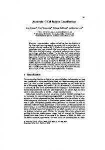
Fig. 1. Two data collection methods: a) collecting the fingerprints at the 15 points (indicated by solid dots), b) collecting fingerprints along the 8 paths (indicated by thick solid lines)

at different headings. In [14], the authors use the Gaussian Process Latent Variable Model (GP-LVM) to solve the WiFi SLAM problem and hence determine the latent-space locations of unlabeled signal strength data. Another relevant work is called Walkie-Markie by Shen et al. [16] Walkie-Markie is an indoor pathway mapping system that can automatically reconstruct internal pathway maps of building without any apriori knowledge about the building. Central to Walkie-Markie are the crowdsourced trajectory information (step count, step frequency, and walking direction) as well as WiFi landmarks derived from WiFi scans. Closest to our work is the quick radio fingerprint collection (QRFC) method proposed in [17]. In QRFC, RSS filtering and shaping are used by averaging neighboring readings along a path to compensate for signal variations along a path caused by multi-path, shadowing, and mask effects. The resulting smoothed RSSes are then stored in a database for “nearest neighbor search” with a relational factor in the operational stage. In comparison, GP in our work performs RSS filtering and shaping automatically. Hyperparameters in GP that control the degree of spatial smoothness and temporal variability are determined using the training data. Another line of work considers AP selection for localization. It was found that not all the APs contribute to indoor positioning in fingerprint-based IPS since APs have different beacon intervals and power saving mode. Previous studies show that judiciously selecting a subset of APs can improve the positioning accuracy (e.g., among those with strongest RSSes) and 6 to 10 APs distributed around the area are often sufficient efficient [15], [18]. AP selection schemes are complementary to fingerprint collection as we generally have no control over when RSSes can be collected from an AP. The former can be used during both the training and operational stages of fingerprint-based localization, and is adopted in TuRF as well. III. S YSTEM OVERVIEW The basic fingerprint-based localization problem consists of determining a device’s position v = (x1 , x2 , ..., xd ) ∈ Rd , given multiple RSS observations s = (s1 , s2 , ..., sm ) ∈ Rm from m APs. This is accomplished by collecting many RSSes from known locations from the target environment and train a

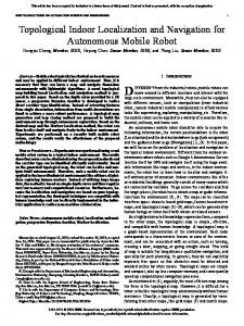
model, also called fingerprint map, that characterizes the functional dependency between the RSS space and the coordinate space, e.g., fi : Rd → R, i = 1, ..., m. Traditionally, site survey for RSS fingerprints is accomplished by first selecting a set of known locations in the target area and then collecting multiple WiFi scans while standing at each location. As an example, in Fig. 1, a fingerprint map can be constructed using RSS vectors collected from the 10 intersecting grid points. TuRF instead collects both WiF RSSes and magnetic field data during walks along predefined trajectories with known starting and ending locations. In Fig. 1, fingerprints are collected opportunistically along the 7 paths (indicated by thick solid lines). Several pertinent questions need to be resolved in utilizing path-based collections in training fingerprint map. 1) How to infer the location tags for the unlabeled fingerprints collected during walking? 2) How fast the walks can be? 3) How to train fi ’s from the fingerprints collected during walking? In the beginning of data collection, a set of paths are predefined. During walks, we only know exactly the locations of the starting and ending points. RSSes contained in WiFi management frames from different APs are captured opportunistically at unknown locations during the walk. In our experiments, a single WiFi scan on an Android device takes about 1s. Human step frequency is around 2Hz. Thus, multiple RSS readings can be captured during one step; and multiple steps are taken during one complete scan. The system architecture of TuRF is given in Fig. 2. The proposed fast site survey process can be further divided into three steps: 1) raw data collection, 2) post processing and 3) model training. In Step 1, the WiFi interface and the magnetometer sensor on a user device are utilized to collect fingerprints with timestamps. The accelerometer sensor data are used for step detection. The timestamps of all step events are recorded. In Step 2, the step events and fingerprints are fused using their respective timestamps. A stride length based location tagging scheme is devised to assign location tags to the collected fingerprints. In Step 3, given the fingerprints with location tags, we train one Gaussian process model for each AP. IV. T U RF L OCATION TAGGING AND T RAINING In this section, we present the details of TuRF location tagging and training processes. For the ease of presentation, we only consider straight-line trajectories. Paths with turns can be broken into line segments using gyroscope readings and handled similarly. A. Location Tagging of Fingerprints Given a predefined path p with length L. Its endpoints are denoted as locstart and locend . A sequence of fingerprints h(f p0 , t0 ), (f p1 , t1 ), · · · , (f pn , tn )i are collected along this path, where f p is a vector of RSS from different access points and/or magnetic filed magnitude. For any hf pi , ti i, our

WIFI

Magnetometer

Accelerometer Step Counter

Step 1:

Step Event with timestamp

Fingerprints with timestamp

Step 2:

Stride Length-Based Location Tagging

Map

Fingerprints with Location Tags Step 3:

Gaussian Process Fig. 2. System Architecture

goal is to infer where it was observed (i.e., its location tag). In this section, we discuss two different location inference approaches, e.g., constant speed based and constant stride length based. Constant speed: In order to infer the collector’s location at time ti along path p, we can simply assume a constant walking speed. The user’s location at ti can be simply calculated by ti − tstart × (locend − locstart ), (1) loci = locstart + tend − tstart where tstart and tend indicate the moments when the user starts and stops walking on p and when the operations are element-wise addition, subtraction and multiplication in the coordinate space. This approach is straightforward but is sensitive to variability in walking speed and stops during walking when encountering obstacles. In order to accommodate the speed variations during walking, we next propose a step-based algorithm. Constant stride length: As discussed in Section III, we use accelerometer in the data collection process for step detection. The step events are utilized to provide better location inference. Let L = |locend −locstart |. Given the timestamps of step events ht01 , t02 , · · · , t0K i, the constant stride length is calculated L as SL = K . Therefore, the user’s location at ti can be further inferred by loci = locstart +

ti −t0j 0 j+1 −tj

j · SL + SL t0 L

× (locend − locstart ) (2)

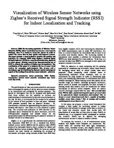
where t0j ≤ ti ≤ t0j+1 . Fig. 3 illustrates the second approach. In the figure, there are 5 steps events and 4 fingerprints are along the path. Therefore, the stride length is estimated L5 . Since the third fingerprint is collected during the fourth step, the location tag of the third fingerprint can be inferred as 3+

t6 −t5 t7 −t5

× (locend − locstart ) (3) 5 Obviously, a robust step counter is crucial to accurate location inference. Step counting is a core module in PDR locstart +

𝐿

TABLE II T HE COLLECTED FINGERPRINTS BY PATH - BASED DATA COLLECTION

𝑆𝐿 𝑆𝐿

Fingerprints Scan

𝑡6 − 𝑡5 𝑡7 − 𝑡5

PROCESS

Step Event

Time

𝑡0 𝑡1

𝑡2

𝑡3 𝑡4

𝑡5

𝑡6 𝑡7

𝑡8

𝑡9

𝑡10

Fig. 3. The location tagging for unlabeled fingerprints

Fingerprints (bssid1 , rss1 ) .. . (bssidi , rssi ) (bssidi+1 , rssi+1 ) .. . (bssidj , rssj ) .. . (bssidN , rssN )

Location loc1 .. . loci loci+1 .. . locj .. . locN

WiFi Scan ID 1 .. . 1 2 .. . 2 .. . N

TABLE I T HE COLLECTED FINGERPRINTS BY TRADITIONAL POINT- BASED DATA COLLECTION PROCESS

Fingerprints Vector h(bssid10 , rss10 ), (bssid11 , rss11 ), · · · i h(bssid20 , rss20 ), (bssid21 , rss21 ), · · · i .. . N N N h(bssidN 0 , rss0 ), (bssid1 , rss1 ), · · · i

Location loc1 loc2 .. . locN

WiFi Scan ID 1 2 .. . N

based IPS [3]. During one step cycle, a person’s body goes through “stance state” with both feet on the ground, and the “swing state” when only one foot is on the ground. As gaits are nearly periodic, steps can be detected by identifying peak accelerations in vertical, forward or lateral directions. Let the 3-axis accelerometer readings at time t be accx (t), paccy (t), accz (t). We first compute the magnitude acc(t) = accx (t)2 + accy (t)2 + accz (t)2 . Then, a low pass filter is applied to remove high-frequency components[19] from the signal. Lastly, a two-threshold based peak detection mechanism is applied to detect step event. Specially, a peak is identified as a step event if the two conditions are met, namely, i) the time difference between two adjacent steps must be greater than a chosen threshold, and ii) the magnitude difference between the adjacent peak and valley must be greater than a chosen threshold. B. Model Training The outputs of site survey and location tagging are a set of fingerprints with (inferred) locations. Given a set of collected fingerprints F P = {(x1 , y1 ), (x2 , y2 ), · · · , (xn , yn )}, where bssidj yi = hyibssid0 , yibssid1 , · · · i where yi indicates the RSS of access point bssidj , observed at location xi . The fingerprintbased indoor localization problem can be formally defined as: Given a set of observations F P , and an incoming y ∗ , how to predict x∗ ? Depending on the fingerprint collection mechanism, the size of collected fingerprints might vary. For example, the fingerprints collected by traditional point-based method is given in Table I, where a fingerprint vector consists multiple elements one from each AP observed. In contrast, the fingerprints collected by the proposed method is in fact a scalar value as illustrated in Table II. Using the data in Table I we can easily train a regression model with multi-dimensional outputs

with missing values imputed 2 . However, this is not the case for the collected fingerprints in Table II. In this work, we assume that the RSS of different access points are independent to each other and a Gaussian process regression model will be trained separately for each access point. Formally, given F P ∗ ∗ and y ∗ = hy bssid0 , y bssid1 , · · · i, x∗ can be estimated as  Y  ∗ x∗ = arg max p y bssidi |x (4) x∈X

i

Now, we are in the position to discuss how to use Gaussian process to calculate the marginal likelihood p(y|x). A Gaussian process can be thought of as a Gaussian distribution over functions (thinking of functions as infinitely long vectors containing the value of the function at every input). Formally, let the input space X and f : X → R a function from the input space to the reals, then we say f is a Gaussian process if for any vector of inputs x = [x1 , x2 , · · · , xn ]T such that xi ∈ X for all i, the vector of output f (x) = [f (x1 ), f (x2 ), ..., f (xn )]T is Gaussian distributed. The Gaussian process is specified by a mean function µ : X → R, such that µ(x) is the mean of f (x) and a covariance (kernel) function k : X × X → R such that k(x, x0 ) is the covariance between f (x) and f (x0 ). We say f ∼ GP (µ, k) if for any x1 , x2 , · · · , xn ∈ X , [f (x1 ), f (x2 ), · · · , f (xn )]T is Gaussian distributed with mean [µ(x1 ), µ(x2 ), · · · , µ(xn )]T and n × n covariance/kernel matrix K:   k(x1 , x1 ) k(x1 , x2 ) · · · k(x1 , xn )  k(x2 , x1 ) k(x2 , x2 ) · · · k(x2 , xn )   K= (5)  ··· ··· ··· ···  k(xn , x1 ) k(xn , x2 ) · · · k(xn , xn ) In our model, we utilize the exponential kernel k(x, x0 ) = σf2 exp(−kx − x0 k/l) where σf2 is the signal variance of f (X) and l is the length scale of the kernel. In Gaussian process, the marginal likelihood is the integral of the likelihood times the prior Z p(y|X) = p(y|f, X)p(f |X)df (6) Under the zero-mean Gaussian prior assumption that f |X ∼ N (0, K) and the likelihood is a factorized Gaussian y|f ∼ 2 One common way for imputing missing values in RSS vectors is to set the corresponding entry to the lowest possible readings, e.g., -93dBm

N (f, σn2 I) where I is an identity matrix and σn2 is the noise variance, we can obtain the log marginal likelihood as

Algorithm 1: BSSIDSelection Input : BSSIDs = {bssid1 , bssid2 , · · · }, 1 > 2 −1 GP Rs : a set of GP regression models logp(y|X) = − y (K + σn I) y 2 θσ : the threshold for noise variance, 1 2 θrss : the threshold for RSS value, (7) − log|K + σn I| 2 θnum : the threshold for number of valid bssids n − log2π. for each position 2 Output: A list of valid bssids The limited-memory BroydenFletcher-Goldfarb-Shanno (LM- 1 validBSSIDs = BSSIDs; BFGS) method is employed to implement this Gaussian pro- 2 sort BSSIDs based on noise variance in descending cess regression. Please refer to [20] for more details. order; 3 foreach bssidi ∈ BSSIDs do C. WiFi RSS fingerprint selection 4 σn2 = bssidi .σn2 ; Nowadays, WiFi has been deployed in almost all the indoor /* Step 1 */ environments. As a result, we can always detect many access 5 if σn2 ≤ θσ then points. The effect of redundant WiFi access point is double6 isDiscarded = False; sided. On the one hand, ubiquitous WiFi infrastructure implies 7 else great potential for WiFi RSS based indoor localization. On 8 isDiscarded = True; the other hand, too many WiFi access points can actually /* Step 2 */ compromise the localization performance, especially for those 9 foreach x ∈ X do whose WiFi signals are poor. In this sense, we need a AP 10 count = 0; selection process to differentiate the “good” and “bad” access 11 foreach bssidj ∈ validBSSIDs do points for indoor localization. We propose a AP selection 12 f = f bssidj ; // get the GPR algorithm, as described in Algorithm 1. It works as follows: 13 rss = f (x); First, all the detected BSSIDs are pre-screened based on their 14 if rss ≥ θrss then noise variances and a noise variance threshold θσ . Then, all the 15 count++; BSSIDs are further assessed based on the number of “good” 16 end (based on a RSS threshold θrss ) BSSIDs at each location and a 17 end threshold θnum . A BSSID might be discarded in noise variance 18 if count < θnum then based pre-screening process, but it will still be retained if 19 isDiscarded = False; it is among the top-θnum BSSIDs at some locations. After 20 end the BSSID selection process, a set of valid BSSIDs will be 21 end generated. In the operational stage, a user observes a set of 22 end fingerprints and submits a location query. Among the observed 23 if isDiscarded == True then BSSIDs, only the valid ones will be used for localization, as 24 remove bssidi from validBSSIDs; elaborated in Algorithm 2. 25 end 26 end V. P ERFORMANCE E VALUATION 27 return validBSSIDs; To evaluate the performance of TuRF, real world experiments are conducted on the second floor of the Information Algorithm 2: Localization Technology Building, McMaster University. Fig. 4 shows the Input : Observations = {(bssid1 , rss1 ), · · · }, floor plan the evaluation area. The area is around 500m2 with GP Rs : a set of GP regression models, dimension 69m by 54m. Both training and testing fingerprints validBSSIDs : output of BSSIDSelection are collected using a Nexus 5 smart phone in the corridors. No Output: Predicted location infrastructure changes were observed during the experiments. 1 observedBSSIDs = {bssids in Observations}; Most of the experiments are conducted during working hours
Q ∩ observedBSSIDs; with people walking around the area. An Android App was 2 BSSIDs = validBSSIDs bssid 3 return arg maxx∈X p y |x bssid∈BSSIDs implemented in Android for raw data collection and step detection. All data post-processing modules are implemented in Python based on open source data science libraries are used, such as Numpy, GPy, and Pandas [21], [22], [23]. during data collection in the evaluation area. After running the In order to make WiFi scan faster, the WiFi interface on AP selection process described in Algorithm 1, a total of 33 the phone is locked to 2.4 GHz using Android API. After BSSIDs are selected. In the experiments, 33 WiFi RSS features band locking, a complete WiFi scan takes between 360ms along with 2 magnetic features are utilized. As discussed in and 420ms. In the evaluation area, there are 21 APs from Section IV, a Gaussian process regression model is trained for our campus networks. 22 other BSSIDs are also observed each feature, separately.

 :DONLQJ 6WDQGLQJ

566G%

    























'LVWDQFHP Fig. 5. RSS comparison between point-based and path-based data collection method

Fig. 4. The floor plan of the evaluation area. Red dots represent the locations selected for point-based data collection whereas the blue line segments are the predefined paths for path-based data collection TABLE III T HE DESCRIPTION OF COLLECTED FINGERPRINTS Data Type Point-based Training data Path-based Training data (Normal speed) Test data

# of path/point 338 points 12 paths

# of WiFi scan 10140 2335

74 points

4440

For comparison, we collect the training data in two ways: point-based data collection, where the user stands at each of the data collection points to collect multiple scans; and the path-based data collection in TuRF, where the user walks in two directions along a set of predefined paths. The evaluation area is divided into 1.2m × 1.2m grids and a total 338 points (red points in Fig. 4) are selected for point-based data collection. The blue lines on Fig. 4 correspond to the paths for walking data collection. The distance between two parallel paths is about 1m. There are a total number of 12 predefined paths. 74 test points were selected evenly spread across the evaluation area, and testing data were collected using the point-based method. The datasets are summarized as Table III. RSS variations during walking: In this experiment, we evaluate signal variations due to the shadowing effect of human body, movement and multi-path induced fading during walking. We select a 10m path and collect RSSes from the same AP using both methods. In the point-based method, RSS are collected from 11 evenly distributed locations along the path. In the path-based method, the user walks slowly along the path at roughly 0.9m/s. Fig. 5 depicts the collected RSS by two different methods. The blue dots indicate the the mean RSS of 30 WiFi scans and the corresponding vertical

bar represents the RSS value range (min and max) at each measuring point. The red dots represent the RSS collected during walking and the locations of these RSSes are inferred by constant stride length based location tagging discussed in Section IV. From Fig. 5, we see that most of the RSSes observed during walking fall in the range of RSSes collected when standing. The location tags inferred from constant stride length appear to work well. Fig. 5 provides a clear insight as to why path-based data collection works – it trades off scans collected per location with scans from more locations. Gaussian process regression: For each of the 35 features, one Gaussian process model was trained using the training data. The hyper parameters (σn , σf , l) are estimated by maximizing the marginal log-likelihood of the training data. We limit the range of noise variance σn between 0.00001 and 9. The GPy framework is used in the optimization process [22]. The resulting GP generates a map with 0.1m × 0.1m grids to be used for localization. The data collected from one AP during normal walking speed is shown in Fig. 7. The colored dots indicate the data collected during walking. We impute missing data using -93 dBm if there is no RSS collected within 6 meter. Fig. 6 shows the mean RSS value prediction using GP. The mean RSS value changes smoothly over the evaluation area. The predicted mean RSS value is close to the RSS observed during walking. Required time for site survey: The total time for site survey can be broken down into i) setup time, during which markers, starting and ending points of paths are decided and measured, and ii) data collection time. Table IV summarizes the setup and data collection times for different data collection methods. In TuRF, it takes us 15 minutes to measure the evaluation area and get the coordinates of the endpoints of predefined paths. For comparison, we ask the user to walk back and forth along each path at slow, normal, fast speed, respectively. It takes another 16, 27, 46 minutes to finish the data collection when the user walks at fast, normal and slow speeds, respectively.

TABLE IV T IME S PENT ON F INGERPRINT C OLLECTION

75.0 77.5 80.0 82.5 85.0 87.5 90.0 92.5

0 10 20 30 40 50 60 70

0

10

20

30

40

50

60

Point-based, 1 WiFi scan at each marker Point-based, 10 WiFi scans at each marker Point-based, 30 WiFi scans at each marker TuRF, walk in fast speed TuRF, walk in normal speed TuRF, walk in slow speed

•

Fig. 6. The mean RSS value prediction using GP for one AP

Data

•

•

50 40

•

30 20

•

10 0 0

10

20

30

40

50

60

Fig. 7. The mean predicted RSS value and training data of one AP

Therefore, the total times needed for data collection, when the user walks in fast, normal, and slow speed, are respectively, 31, 42, and 61 minutes. This is in contrast to data collection using the point-based method. It takes 120 minutes to measure the evaluation area and setup the markers. The total times for data collection, when 1, 10 and 30 WiFi scans are collected at each marker, are respectively, 67, 135, and 270 minutes. As shown in Table IV, TuRF reduces both the setup time and the data collection time significantly. Another potential benefit of path-based data collection is that the few endpoints of paths are much easier to maintain for future fingerprint update compared to hundreds of markers needed for point-based data collection if the markers are accidentally damaged or removed. Localization performance: In this experiment, we compare the localization accuracy using the training data collected by point-based data collection and TuRF. We also evaluate the impacts of location tag inference methods, walking speed and magnetic features. Six variants of the combined techniques are evaluated. •

WiFi+speed: Only WiFi RSS fingerprints are used. The location tagging is based on constant speed.

Setup Time 120 minutes

Data Collection Time 67minutes

120 minutes

135 minutes

120 minutes

270 minutes

15 minutes 15 minutes 15 minutes

16 minutes 27 minutes 46 minutes

WiFi+stride: Only WiFi RSS fingerprints are used. The location tagging is based on constant stride length. WiFi+magnetic1+speed: Both WiFi RSS and magnetic field magnitude are used as fingerprints. The location tagging is based on constant speed. WiFi+magnetic1+stride: Both WiFi RSS and magnetic field magnitude are used as fingerprints. The location tagging is based on constant stride length. WiFi+magnetic2+speed: Both WiFi RSS, magnetic field magnitude and magnetic field magnitude on Z-axis are used as fingerprints. The location tagging is based on constant speed. WiFi+magnetic2+stride: Both WiFi RSS, magnetic field magnitude and magnetic field magnitude on Z-axis are used as fingerprints. The location tagging is based on constant stride length.

The results are depicted as Fig. 8. The red horizontal line indicates the performance of point-based data collection algorithm in which both WiFi and magnetic fingerprints are utilized. The vertical bars represent the localization performances of path-based data collection methods. A few observations are in order from Fig. 8. First, localization results from the constant stride length based location tagging algorithm are constantly better than those from the constant speed based algorithm in all the cases. This indirectly confirms that location tags using constant stride length are likely to be more accurate. Second, incorporation of magnetic fingerprints can indeed improve the localization performance. Using both magnetic features are beneficial. Third, when constant stride length location tagging is used, TuRF outperforms point-based data collection when the walking speed is slow and normal. Recall from Table III, the total numbers of WiFi scans in the point-based method and TuRF at the normal walking speed are 10140 and 2335, respectively. With fewer scans, the superior performance of TuRF can be attributed to denser spatial sampling. Fourth, as expected, slower walking speeds allow collection of fingerprints and thus lead to better localization accuracy. Walking speed recommendation: As shown in Fig. 8, we observe that lower walking speed leads to better localization performance in TuRF. However, there exists a trade-off between the time spent on site survey and localization accuracy. Through extensive experiments, we find that a reasonable localization performance can be attained if there are one or

/RFDOL]DWLRQ(UURUP



ZLILVSHHG ZLILVWULGH

ZLILPDJQHWLFVSHHG ZLILPDJQHWLFVWULGH

ZLILPDJQHWLFVSHHG ZLILPDJQHWLFVWULGH









VORZ

QRUPDO

IDVW

Fig. 8. Comparison of different strategies, walking speeds, features and location tagging approaches TABLE V WALKING SPEED RECOMMENDATION FOR DIFFERENT DEVICES Device Nexus 5 Samsung Galaxy Note 3 Samsung Galaxy S4 Samsung Galaxy Mini III

Required time for one WiFi Scan 380 ms 1420 ms 780 ms 1150 ms

Recommended walking speed 2.63 step/s 0.70 step/s 1.28 step/s 0.87 step/s

more WiFi scans that can be done within one step. Based on this observation, the recommended walking speed is given by, 1 (8) tW iF iScan The amount of time for one WiFi scan is both device and configuration dependent. Rule-of-thumb walking speed recommendations for different Android devices are given in Table V. recommended walking speed ≤

VI. C ONCLUSION In this paper, we presented TuRF, a fast path-based data collection method for fingerprint collection. The Gaussian process regression model was utilized to provide a flexible model training process for localization. Experimental results demonstrated the efficiency and effectiveness of the proposed method. We found that TuRF can indeed reduce the required time for site survey without sacrificing localization performance. As future work, we are interested in incremental fingerprints updating strategies and investigate the adaptive data collection approaches where users are promoted if walk speeds shall be adjusted and revisits to some areas are required. R EFERENCES [1] Z. Yang, C. Wu, and Y. Liu, “Locating in fingerprint space: wireless indoor localization with little human intervention,” in Proceedings of the 18th annual international conference on Mobile computing and networking. ACM, 2012, pp. 269–280. [2] G. B. Prince and T. D. Little, “A two phase hybrid RSS/AoA algorithm for indoor device localization using visible light,” in Global Communications Conference (GLOBECOM). IEEE, 2012, pp. 3347–3352.

[3] Q. Xu, R. Zheng, and S. Hranilovic, “Idyll: Indoor localization using inertial and light sensors on smartphones,” in Proceedings of the 2015 ACM International Joint Conference on Pervasive and Ubiquitous Computing, ser. UbiComp ’15. New York, NY, USA: ACM, 2015, pp. 307–318. [4] A. Rai, K. K. Chintalapudi, V. N. Padmanabhan, and R. Sen, “Zee: zeroeffort crowdsourcing for indoor localization,” in Proceedings of the 18th annual international conference on Mobile computing and networking. ACM, 2012, pp. 293–304. [5] Q. Xu and R. Zheng, “Mobibee: A mobile treasure hunt game for location-dependent fingerprint collection,” in Proceedings of the 2016 ACM International Joint Conference on Pervasive and Ubiquitous Computing: Adjunct, ser. UbiComp ’16. New York, NY, USA: ACM, 2016, pp. 1472–1477. [6] C. Peng, G. Shen, Y. Zhang, Y. Li, and K. Tan, “Beepbeep: a high accuracy acoustic ranging system using cots mobile devices,” in Proceedings of the 5th international conference on Embedded networked sensor systems. ACM, 2007, pp. 1–14. [7] K. Liu, X. Liu, and X. Li, “Guoguo: Enabling fine-grained indoor localization via smartphone,” in Proceeding of the 11th annual international conference on Mobile systems, applications, and services. ACM, 2013, pp. 235–248. [8] J. Xiong and K. Jamieson, “Arraytrack: A fine-grained indoor location system.” in NSDI, 2013, pp. 71–84. [9] P. Bahl and V. N. Padmanabhan, “Radar: An in-building rf-based user location and tracking system,” in INFOCOM 2000. Nineteenth Annual Joint Conference of the IEEE Computer and Communications Societies. Proceedings. IEEE, vol. 2. Ieee, 2000, pp. 775–784. [10] R. Harle, “A survey of indoor inertial positioning systems for pedestrians.” IEEE Communications Surveys and Tutorials, vol. 15, no. 3, pp. 1281–1293, 2013. [11] Y. Li, Z. He, J. Nielsen, and G. Lachapelle, “Using wi-fi/magnetometers for indoor location and personal navigation,” in Indoor Positioning and Indoor Navigation (IPIN), 2015 International Conference on. IEEE, 2015, pp. 1–7. [12] J. Chung, M. Donahoe, C. Schmandt, I.-J. Kim, P. Razavai, and M. Wiseman, “Indoor location sensing using geo-magnetism,” in Proceedings of the 9th international conference on Mobile systems, applications, and services. ACM, 2011, pp. 141–154. [13] V. Guimar˜aes, L. Castro, S. Carneiro, M. Monteiro, T. Rocha, M. Barandas, J. Machado, M. Vasconcelos, H. Gamboa, and D. Elias, “A motion tracking solution for indoor localization using smartphones,” in Indoor Positioning and Indoor Navigation (IPIN), 2016 International Conference on. IEEE, 2016, pp. 1–8. [14] B. Ferris, D. Fox, and N. D. Lawrence, “Wifi-slam using gaussian process latent variable models.” [15] C. Feng, W. S. A. Au, S. Valaee, and Z. Tan, “Received-signal-strengthbased indoor positioning using compressive sensing,” IEEE Transactions on Mobile Computing, vol. 11, no. 12, pp. 1983–1993, 2012. [16] G. Shen, Z. Chen, P. Zhang, T. Moscibroda, and Y. Zhang, “Walkiemarkie: indoor pathway mapping made easy,” in Proceedings of the 10th USENIX conference on Networked Systems Design and Implementation. USENIX Association, 2013, pp. 85–98. [17] H.-H. Liu, “The quick radio fingerprint collection method for a wifibased indoor positioning system,” Mobile Networks and Applications, pp. 1–11, 2015. [18] M. A. Youssef, A. Agrawala, and A. U. Shankar, “Wlan location determination via clustering and probability distributions,” in Pervasive Computing and Communications, 2003.(PerCom 2003). Proceedings of the First IEEE International Conference on. IEEE, 2003, pp. 143–150. [19] R. Libby, “A simple method for reliable footstep detection in embedded sensor platforms.(2012),” 2012. [20] R. H. Byrd, P. Lu, J. Nocedal, and C. Zhu, “A limited memory algorithm for bound constrained optimization,” SIAM Journal on Scientific Computing, vol. 16, no. 5, pp. 1190–1208, 1995. [21] S. v. d. Walt, S. C. Colbert, and G. Varoquaux, “The numpy array: a structure for efficient numerical computation,” Computing in Science & Engineering, vol. 13, no. 2, pp. 22–30, 2011. [22] GPy, “GPy: A gaussian process framework in python,” http://github. com/SheffieldML/GPy, since 2012. [23] W. McKinney et al., “Data structures for statistical computing in python,” in Proceedings of the 9th Python in Science Conference, vol. 445. van der Voort S, Millman J, 2010, pp. 51–56.