in a new space which must include smooth (low-pass) components. As such, we can effectively interpolate the smooth components with fast linear interpolators,.
FAST EDGE-GUIDED INTERPOLATION OF COLOR IMAGES
Keywords:
Color images, interpolation, real-time applications.
Abstract:
We propose a fast adaptive image interpolation method for still color images which is suitable for real-time applications. The proposed interpolation scheme combines the speed of fast linear image interpolators with advantages of an edge-guided interpolator. A fast and high performance image interpolation technique is proposed to interpolate the luminance channel of low-resolution color images. Since the human visual system is less sensitive to the chrominance channels than the luminance channel, we interpolate the former with the fast method of bicubic interpolation. This combinatory technique achieves high PSNR and superior visual quality by preserving edge structures well while maintaining a low computational complexity. As verified by the simulation results, interpolation artifacts (e.g. blurring, ringing and jaggies) plaguing linear interpolators are noticeably reduced with our method.
1
INTRODUCTION
Image interpolation has been an active research topic since early days of image processing, due to a wide range of its applications, including resolution upconversion, resizing, video deinterlacing, video frame rate upconversion, subpixel motion estimation, image compression, etc. Many of these applications have real-time requirements, for examples, video deinterlacing and resolution or/and frame rate upconversion. The common solutions for real-time image interpolation are simple image-independent linear filters, such as bilinear interpolator and bicubic interpolator (Keys, 1981). But these simple linear filters are isotropic and ill suited for directional image waveforms and also cannot cope with the nonlinearities of the image formation model (Plataniotis et al., 1999). Hence they tend to produce severe interpolation artifacts in areas of edges and fine image details. To overcome the above said weaknesses of signalindependent isotropic interpolators, adaptive nonlinear interpolators were introduced (Li and Orchard, 2001), (Muresan, 2005), (Zhang and Wu, 2006) and (Li and Nguyen, 2008). Among these algorithms, edge preserving interpolators are of great interest.
The ultimate goal of an edge-guided image interpolation technique is to avoid interpolation against the existing edge directions for each missing highresolution (HR) pixel. This achieves clean and sharp reproduced edges in the HR output image. However in practice there is a major issue with most of the developed edge-guided interpolators. The edgeguided interpolators achieve better perceptual quality than linear filters at cost of higher computational complexity. Therefore most of these algorithms are not suitable for real-time applications. In this work, we address this issue and propose a fast and high-performance edge-guided interpolation algorithm for color images. In the proposed algorithm, low-resolution (LR) color images are converted to the luminance-chrominance space, from the RGB counterpart and the interpolation process is carried out in the new space. The reason for this mapping is twofold. First, the human visual system is much less sensitive to the chrominance components than the luminance. Hence, we apply a sophisticated interpolation technique to interpolate the luminance channel and for computational savings, a simple linear filter e.g. bicubic is applied for the chrominance channels. Second, the luminance channel captures the variations
in the image and magnifies the edges and other highfrequency components. This achieves higher reliability on the extracted edge information from the LR image, which is crucial for directional image interpolation. To interpolate the luminance channel, we also propose a fusion-based image interpolation method. As verified by the simulations, this technique achieves superior performance than the competing methods, at lower computational complexity. The presentation of this paper is as follows. The proposed interpolation scheme for color images is described in section. 2. Proposed edge-guided interpolation algorithm for gray-scaled images is presented in section.3. Section.4 presents the simulation results and section.5 concludes.
2
PROPOSED ALGORITHM FOR COLOR IMAGE INTERPOLATION
As in the existing literature, we assume that each pixel in the input color image has three color values: red (R), green (G) and blue (B). In pursuit of low computational cost, we interpolate color images in a new space which must include smooth (low-pass) components. As such, we can effectively interpolate the smooth components with fast linear interpolators, without sacrificing the perceptual quality. The convenient RGB to YCbCr conversion faithfully satisfy the above condition. The equations for this mapping in the JPEG JFIF format (Hamilton, 1992) are: = = =
Y Cb Cr
0.299R + 0.587G + 0.114B −0.1687R − 0.3313G + 0.5B 0.5R − 0.4187G − 0.0813B
= Y + 1.402Cr = Y − 0.34414Cb − 0.71414Cr = Y + 1.772Cb
(2)
However, the applied coefficients in (1) and (2) are real numbers which incurs error for hardware implementations. This issue can be addressed by applying a reversible transformation such as RGB to YCoCg with corresponding conversion formula: Y Co Cg
= = =
0.25R + 0.5G + 0.25B 0.5R − 0.5B −0.25R + 0.5G − 0.25B
R = Y + Co − Cg G = Y + Cg B = Y − Co − Cg.
(4)
For more details about developing of (3) and (4) please refer to (Malvar et al., 2008). The advantage of YCoCg transform over YCbCr is that the inverse formula, mapping YCoCg into RGB only requires additions and subtractions. To be more precise, the inversion can be performed with four additions: G = Y + Cg, t = Y − Cg, R = t + Co and B = t − Co (Malvar et al., 2008). We use this reversible transformation for the proposed interpolation technique. Color images are converted from RGB to YCoCg space, then the chrominance channels (Co and Cg) are interpolated with bicubic interpolator. By now, we have described the interpolation process of the chrominance channels. Human visual system is more sensitive to the luminance (Y) channel. Hence in our design a high-performance edge-guided interpolation algorithm is utilized for interpolation of the luminance channel. In the next section the proposed image interpolation algorithm for the Y channel is presented.
3
FAST ADAPTIVE INTERPOLATION OF GRAY-SCALED IMAGES
(1)
and the reverse equations are given as: R G B
and reverse formula
(3)
Figure 1: (a) Formation of a high-resolution (HR) image from low-resolution (LR) samples (empty circles) and missing HR pixels (black circles). (b),(c) Interpolation of HR missing pixels with different coordinates. Two estimates are made from the LR samples (hatches circles) for each missing pixel.
In this section we reexamine the problem of resolution upconversion of gray-scaled images. Formation of an HR image from original LR samples is depicted in figures. 3(a). The missing pixels are recovered in two batches. First missing pixels with coordinates (2i, 2 j) are recovered and in the second batch, pixels with coordinates (2i − 1, 2 j) and (2i, 2 j − 1) are interpolated. As illustrated in figures. 3(b) and (c), the problem of
31.2 31.15 31.1
PSNR
31.05 31 30.95 30.9 30.85 30.8 30.75 0
5
10
15
|γ|
Figure 2: Average PSNR result over a set of training images for different values of γ.
interpolation of the second batch becomes the same as the first bacth by 45◦ rotation. Therefore, we only describe the algorithm for the first batch in detail. Two directional estimates for each missing pixel are obtained by cubic convolution (Keys, 1981): d1 and d2 (figures. 3(b) and (c)). In (Zhang and Wu, 2006) a linear minimum mean-squares method of fusing these two directional estimates is proposed. For low complexity and ease of implementation, we also adopt affine weights to linearly fuse d1 and d2 to interpolate the HR pixel YHR , namely: YHR = αd1 + (1 − α)d2, α ∈ [0, 1].
(5)
The value of α is computed as follows. First, the smoothness along directions 1 and 2 are measured by computing the sum of the absolute differences (SAD) of the available LR pixels in the locality of the missing HR pixel YHR (2i, 2 j) as: SAD1 (2i, 2 j) = ∑ YLR (m, n) −YLR (m + 1, n + 1) (m,n)∈W2i,2 j
(6)
and SAD2 (2i, 2 j) =
∑
YLR (m, n) −YLR (m − 1, n + 1)
Figure 3: Six sample images in the test set: (a) Lena, (b) Parrots, (c) Flight, (d) Window, (e) Flower and (f) Fruits.
3.1 calculation of γ In our design, the value of γ is determined by training. A large set of HR images is selected and downsampled by the factor of two and then reconstructed by the proposed method. The training is accomplished on the activity regions of the aforementioned HR images. The average PSNR over the all training images for different values of γ is plotted in figures 2. We choose γ = −4 that achieves the highest objective performance for the proposed method.
4
SIMULATION RESULTS
The proposed interpolation method was implemented and tested on a variety of scenes. A brief objective comparison between the proposed method in section.3 and some existing interpolation algorithms is presented by Table 1. Please note that the reported PSNR results are for the luminance channel of the
(m,n)∈W2i,2 j
(7)
where W2i,2 j is a 7 × 7 spatial template in the HR lattice centered at the position (2i, 2 j). As described in the section.1, edge-guided interpolators perform the interpolation filtering along the directions of smoothness. Hence, it is expected that more wight be assigned to the direction with less corresponding value γ of SADk , which means: αˆ ∝ SAD1 , γ < 0 in our design. Once γ is given, αˆ is computed as: γ
SAD1 (8) γ γ. SAD1 + SAD2 The following subsection concerns with evaluating the global optimum value of γ for the proposed algorithm. αˆ =
Table 1: PSNR (decibels) results of reconstructed images and the average execution time for NEDI (Li and Orchard, 2001), LMMSE INTR (Zhang and Wu, 2006) and the proposed method.
Image Lena Parrot Flight Window Bush Fruits Average Time(s)
NEDI 33.36 34.52 29.95 34.68 27.96 36.35 32.80 21.03
LMMSE INTR 33.38 34.15 29.92 34.92 28.12 36.81 32.88 10.52
Proposed 33.93 35.21 30.36 35.88 28.77 38.92 34.01 0.92
Table 2: PSNR (decibels) results of reconstructed color images in figures. 3 in YCoCg color space with three different methods. bicubic: all channels are interpolated with bicubic. bicubic+proposed: Y channel is interpolated by the proposed method in section. 3 and chrominance channels are interpolated with bicubic. proposed: all channels are recovered with the proposed algorithm in section. 3.
Image channels bicubic bicubic+proposed proposed Image channels bicubic bicubic+proposed proposed
Lena G 32.19 32.70 32.70 Window R G 34.94 34.92 35.61 35.63 35.62 35.62 R 35.47 35.53 35.89
B 30.72 31.07 31.18 B 34.75 35.44 35.37
Parrot G 34.09 34.96 34.92 Bush R G 28.10 27.10 28.15 27.25 28.13 27.19 R 34.13 34.99 34.98
B 34.04 34.89 34.85 B 30.15 29.92 30.25
Flight G 29.54 30.43 30.43 Fruits R G 36.79 37.20 37.45 37.88 37.48 37.91 R 29.69 30.55 30.54
B 29.33 30.20 30.19 B 38.51 38.70 38.87
pictures depicted in figures. 3. As verified by the results, the proposed method outperforms the competition with NEDI (Li and Orchard, 2001) and method of (Zhang and Wu, 2006) which are among the best edge-guided image interpolation algorithms in the literature. The reported execution time also verifies the simplicity of the proposed algorithm. The major parameters of the exploited server for the simulations R are: CPU: Intel Core 2 Duo E8400 (3 GHz), RAM: 4 GB, 6 MB of L2 cache and 1333 MHz front side bus (FSB). The proposed algorithm is highly parallelizable, since it recovers each missing pixel in isolation. Therefore the proposed algorithm is also suitable for hardware implementations. To evaluate the performance of the proposed interpolation scheme for color images we conduct the following test. The color images listed in the figures.3 are first down-sampled by a factor of two, and recovered by three different schemes: 1. bicubic: the R,G and B channels are interpolated with bicubic interpolator. 2. bicubic+proposed: images are first converted to the YCoCg space and the Y channel is upconverted by the proposed edge-guided interpolator while the Co and Cg channels are interpolated by bicubic. 3. proposed: images are first converted to the YCoCg space and the Y,Co and Cg channels are interpolated with the proposed edge-guided interpolator. The results are tabulated in Table.2. It can be verified that the combinatory algorithm (bicubic+proposed) achieves similar results to those of the third algorithm. The perceptual quality of the recovered image by the three algorithms are compared in figures. 4,5 and 6. The outputs of the schemes 2 and 3 are visually sim-
Figure 4: Interpolation results of a portion of the image Fruits with three different methods: (a) bicubic, (b) bicubic+proposed, (c) proposed. (a) is the original image.
ilar which manifests the efficacy of the proposed algorithm for reducing the complexity of color image interpolation without loss of visual quality. The reconstructed images by the proposed simplified image interpolation method are in turn greatly sharper and cleaner than those of bicubic interpolation.
5
CONCLUDING REMARKS
A fast interpolation algorithm for color images is proposed. Color images are first converted from RGB to
waveforms, we can effectively interpolate them without degrading of the perceptual quality of the recovered images. Simulation results verify that the proposed interpolation technique is fast and also removes common interpolation artifacts.
REFERENCES Hamilton (1992). Jpeg file interchange format, version 1.02. Keys, R. G. (1981). Cubic convolution interpolation for digital image processing. In IEEE Trans. Acoustic, Speech, Signal Process. Li, M. and Nguyen, T. Q. (2008). Markov random field model-based edge-directed image interpolation. In IEEE Trans. on Image Processing. Li, X. and Orchard, M. T. (2001). New edge-directed interpolation. In IEEE Trans. on Image Processing.
Figure 5: Interpolation results of a portion of the image Flight with three different methods: (a) bicubic, (b) bicubic+proposed, (c) proposed. (a) is the original image.
Malvar, H. S., Sullivan, G. J., and Srinivasan, S. (2008). Lifting based reversible color transformations for image compression. In SPIE Applications of Digital Image Processing. Muresan, D. D. (2005). Fast edge directed polynomial interpolation. In IEEE International Conference on Image Processing. Plataniotis, K. N., Androutsos, D., and Venetsanopoulos, A. N. (1999). Adaptive fuzzy systems for multichannel signal processing. In Proceedings of the IEEE. Zhang, L. and Wu, X. (2006). An edge-guided image interpolation algorithm via directional filtering and data fusion. In IEEE Trans. on Image Processing.
Figure 6: Interpolation results of a portion of the image Bush with three different methods: (a) bicubic, (b) bicubic+proposed, (c) proposed. (a) is the original image.
luminance-Chrominance format, then the luminance channel is interpolated with a proposed edge-guided interpolation technique and the luminance channels are interpolated with simple bicubic interpolation. Since chrominance channels include low-pass 2D