Fast Fourier Transform Processors: Implementing ... - Semantic Scholar

0 5 Fast Fourier Transform Processors: Implementing FFT and IFFT Cores for OFDM Communication Systems A. Cortés, I. Vélez, M. Turrillas and J. F. Sevillano TECNUN (Universidad de Navarra) and CEIT Spain 1. Introduction The terms Fast Fourier Transform (FFT) and Inverse Fast Fourier Transform (IFFT) are used to denote efficient and fast algorithms to compute the Discrete Fourier Transform (DFT) and the Inverse Discrete Fourier Transform (IDFT) respectively. The FFT/IFFT is widely used in many digital signal processing applications and the efficient implementation of the FFT/IFFT is a topic of continuous research. During the last years, communication systems based on Orthogonal Frequency Division Multiplexing (OFDM) have been an important driver for the research in FFT/IFFT algorithms and their implementation. OFDM is a bandwidth efficient multiple access scheme for digital communications (Engels, 2002; Nee & Prasad, 2000). Many of nowadays most important wireless communication systems use this OFDM technique: Digital Audio Broadcasting (DAB) (World DAB Forum, n.d.), Digital Video Broadcasting (DVB) (ETS, 2004), Wireless Local Area Network (WLAN) (IEE, 1999), Wireless Metropolitan Area Network (WMAN) (IEE, 2003) and Multi Band –OFDM Ultra Wide Band (MB–OFDM UWB) (ECM, 2005). Moreover, this technique is also employed in important wired applications such as Asymmetric Digital Subscriber Line (ADSL) or Power Line Communication (PLC). OFDM systems rely on the IFFT for an efficient implementation of the signal modulation on the transmitter side, whereas the FFT is used for efficient demodulation of the received signal. The FFT/IFFT becomes one of the most critical modules in OFDM transceivers. In fact, the most computationally intensive parts of an OFDM system are the IFFT in the transmitter and the Viterbi decoder in the receiver (Maharatna et al., 2004). The FFT is the second computationally intensive part in the receiver. Therefore, the implementation of the FFT and IFFT must be optimized to achieve the required throughput with the minimum penalty in area and power consumption. The demanding requirements of modern OFDM transceivers lead, in many cases, to the implementation of special–purpose hardware for the most critical parts of the transceiver. Thus, it is common to find the FFT/IFFT implemented as aVery Large Scale Integrated (VLSI) circuit. The techniques applied to the FFT can be applied to the IFFT as well. Moreover, the IFFT can be easily obtained by manipulating the output of a FFT processor. Therefore, the discussion in this chapter concentrates on the FFT without loss of generality.

112

2

Fourier Transform – Signal Processing Will-be-set-by-IN-TECH

Different kinds of FFT algorithms can be found in the literature; e.g.: (Good, 1958; Thomas, 1963), (Cooley & Tukey, 1965), (Rader, 1968b), (Rader, 1968a), (Bruun, 1978) and (Winograd, 1978). Among the different kinds of FFT algorithms, the algorithms based on the approach proposed by James W. Cooley and John W. Tukey in (Cooley & Tukey, 1965) are very popular in OFDM systems. These Cooley–Tukey (CT) algorithms present a very regular structure, which facilitates an efficient implementation. The computations of the FFT is divided into logr ( N ) stages, where N is the number of points of the FFT and r is called the radix of the algorithm. Within each stage, data shuffling and the so-called butterfly computation and twiddle factor multiplications are performed. Usually, the butterfly operations are all identical and the twiddle factor multiplications and data shuffling follow some kind of pattern. This regular structure makes them very attractive for VLSI circuit implementation. Different hardware architectures have been used in the literature for the implementation of the CT algorithms. The FFT hardware architectures can be classified into three groups: • Monoprocessor: A single hardware element is used to perform all the butterflies, twiddle factor multiplications and data shuffling of each stage. The same hardware is reused for all the stages. • Parallel: The computation of the butterflies, twiddle factor multiplications and data shuffling within one stage is accelerated by using several processing elements. The same hardware elements are again reused for all the stages. • Pipeline: A single hardware element is used to perform all the butterflies, twiddle factor multiplications and data shuffling of each stage. However, in contrast to former categories, a different hardware element is used to process each stage. It is common in the literature to further classify the pipeline architectures according to the structure used for the shuffling into two basic types: Delay Commutator (DC) and Delay Feedback (DF). Also, according to the number of lines of data used in these pipeline architectures, they can be classified into Single–path (S) or Multiple–path (M) architectures. Many different variations of CT algorithms have been proposed in the literature to improve different aspects of the implementation (memory resources, number of arithmetic operations, etc.) and their mapping to a specific hardware architecture. Table 1 summarizes the features of some FFT/IFFT processors for OFDM systems proposed in the literature. Proposals such as (Chang & Park, 2004; Serrá et al., 2004) employed a monoprocessor architecture to process the FFT. (Jiang et al., 2004; Lin, Liu & Lee, 2004) used parallel architectures and (Kuo et al., 2003) chose a cached memory monoprocessor architecture for the FFT processing in an OFDM system. However, the most widely used architectures for the FFT/IFFT processor in an OFDM system are pipeline architectures. (Cortés et al., 2007; He & Torkelson, 1998; Lee & Park, 2007; Lee et al., 2006; Turrillas et al., 2010; Wang et al., 2005) propose Single-Path Delay Feedback (SDF) architectures. (Lin et al., 2005; Liu et al., 2007) employ an Multi-Path Delay Feedback (MDF) architecture. (Bidet et al., 1995) proposes a Single-Path Delay Commutator (SDC) architecture and (Jung et al., 2005; Saberinia, 2006) chose an Multi-Path Delay Commutator (MDC) architecture. (Saberinia, 2006) called the MDC architecture as Buffered Multi-Path Delay Commutator (BRMDC) due to the buffers used in the input data. Analyzing the radix, r, of the algorithms employed in the literature, it can be observed that: • For the monoprocessor architectures, radix 2 (Serrá et al., 2004) and radix 4 (Chang & Park, 2004) algorithms have been used.

Fast Fourier Transform Processors: Implementing FFT and IFFT Cores for Cores OFDM Communication Systems Fast Fourier Transform Processors: Implementing FFT and IFFT for OFDM Communication Systems Reference FFT points (Jung et al., 2005) 64 (Maharatna et al., 2004) 64 (Serrá et al., 2004) 64 (Lin et al., 2005) 128 (Saberinia, 2006) 128 (Lee et al., 2006) 128 (Liu et al., 2007) 64/128 (Cortés et al., 2007) 128 (Bidet et al., 1995) 8192 (Lin, Liu & Lee, 2004) 8192 (Wang et al., 2005) 2/8 K (Lenart & Owal, 2006) 2/4/8 K (Lee & Park, 2007) 8K (He & Torkelson, 1998) 1024 (Kuo et al., 2003) 64–2048 (Chang & Park, 2004) 1024 (Jiang et al., 2004) 64 (Lin, Lin, Chen & Chang, 2004) 64 (Rudagi et al., 2010) 64 (Yu et al., 2011) 64 (Tsai et al., 2011) 64 (Turrillas et al., 2010) 32 K

1133

Architecture Algorithm Application Pipeline–MDC r–2 DIT WLAN Pipeline r–2 DIT WLAN Monoprocessor r–2 DIT WLAN Pipeline–MRMDF MR 2/23 DIF UWB Pipeline–BRMDC r–2 DIF UWB Pipeline–SDF r–24 DIF UWB Pipeline 8-path DF MR DIF UWB Pipeline r–24 DIF UWB Pipeline–SDC r–4/2 DIF DVB–T Parallel r–23 DIT DVB–T Pipeline–SDF r–4/2 DIF DVB–T Pipeline–SDF r–22 DIF DVB–T/H Pipeline–SDF BD DVB–T Pipeline–SDF r–22 DIF OFDM Cached memory r–2 DIT OFDM Monoprocessor r–4 DIF OFDM Parallel r–2 DIT OFDM Pipeline r–2 DIF MIMO Pipeline r–2 DIT OFDM Pipeline r–2 DIF OFDM Pipeline MR OFDM Pipeline r–2k DIF DVB–T2

Table 1. FFT proposals for OFDM systems • For the parallel architectures, FFT algorithms such as radix 2 (Jiang et al., 2004) and radix 23 (Lin, Liu & Lee, 2004) have been used. • For the pipeline architectures, different FFT algorithms such as radix 2 (Jung et al., 2005; Rudagi et al., 2010; Saberinia, 2006; Yu et al., 2011), mixed radix (MR) (Bidet et al., 1995; Lin, Lin, Chen & Chang, 2004; Lin et al., 2005; Liu et al., 2007; Tsai et al., 2011; Wang et al., 2005), radix 22 (Cortés et al., 2007; He & Torkelson, 1998; Lenart & Owal, 2006; Turrillas et al., 2010), radix 23 (Cortés et al., 2007; He & Torkelson, 1998; Turrillas et al., 2010), radix 24 (Cortés et al., 2007; Lee et al., 2006; Turrillas et al., 2010) and balanced decomposition (BD) (Lee & Park, 2007) which reduces the number of twiddle factors have been proposed. When the length of the FFT is not very large, the fixed-point format is the most widely used number representation format due to the area-saving with respect to the floating-point representation. Thus, (Chang & Park, 2004; Cortés et al., 2007; He & Torkelson, 1998; Jiang et al., 2004; Jung et al., 2005; Kuo et al., 2003; Lee et al., 2006; Lin, Lin, Chen & Chang, 2004; Lin et al., 2005; Liu et al., 2007; Maharatna et al., 2004; Saberinia, 2006; Serrá et al., 2004) proposed fixed–point FFTs for N < 8192. Nevertheless, (Wang et al., 2005) also used the fixed–point format for large FFTs. However, when the length of the FFT increases, different types of non fixed-point formats have been used. (Bidet et al., 1995) proposed a 8K processor that uses Convergent block floating–point to improve the quantization error of the FFT design. The block floating–point implementation or the semi–floating point (SFlP) format achieve a more efficient FFT design in (Lee & Park, 2007; Lenart & Owal, 2006). In a different approach, (Turrillas et al., 2010) employed a variable datapath technique to process a 32K points FFT.

114

4


From Table 1, it can be seen that many different algorithms and architectures have been proposed for OFDM systems. The designer must select the most appropriate algorithm and the most efficient architecture for that algorithm, given the specifications of a certain OFDM system. This selection is a difficult task. There is not a clear algorithm/architecture winner. Therefore, the designer should explore different algorithms and architectures in the literature to find the optimal one for the specific OFDM application under development. The typical way of expressing the FFT algorithms in the literature is by means of summations or flow graph notation. Examples of these representations can be found in (He & Torkelson, 1998; Lee & Park, 2007; Lee et al., 2006; Lin, Lin, Chen & Chang, 2004; Lin, Liu & Lee, 2004; Lin et al., 2005; Liu et al., 2007; Maharatna et al., 2004; Tsai et al., 2006). These representations do not help the designer to understand the algorithm fast, therefore, making it difficult to relate it to its HW resources. Additionally, sometimes there is a lack of a general expression for the algorithm/architecture, which makes it harder to adapt and evaluate for a different OFDM system. Therefore, these representations are not practical for design space exploration. What the designer needs for efficient design space exploration is a general expression for the different design parameters of the algorithms which is easy to understand and makes it fast to map to hardware resources. In (Pease, 1968), a matrix notation to express the FFT is proposed. Different FFT algorithms are obtained combining a reduced set of operators to simplify the implementation of parallel processing in a special–purpose machine. In (Sloate, 1974), H. Sloate used the same approach as (Pease, 1968) to demonstrate how several FFT algorithms previously defined could be derived using the matricial expressions. Additionally, he analyzed some new algorithms and worked out how to relate the matricial expressions to their implementation. However, that notation is not generalized for pipeline architectures. Recently, (Cortés et al., 2009) generalized the above approach presenting a unified approach for radix r k pipeline SDC/SDF FFT architectures. Radix r k pipeline FFT architectures are very efficient architectures that are well suited for OFDM systems. This chapter reviews the matricial representation of radix r k pipeline SDF FFT architectures. Thus, a general expression in terms of the FFT design parameters that can be linked easily to hardware implementation resources is presented. This way, the designer of FFT/IFFT processors for OFDM systems is provided with the tools for efficient design space exploration. The design space exploration and the optimal architecture selection procedure is illustrated by means of a case study. The case study analyzes the FFT/IFFT processor in a WLAN IEEE 802.11a transceiver. The high level analysis proposed in (Cortés et al., 2009) is extended to implementation level to select the most efficient FFT/IFFT core in terms of area and power consumption.

2. A unified matricial approach for radix r k FFT SDF pipeline architectures This section presents the matricial representation of radix r k Decimation In Frequency (DIF) SDF pipeline architectures. First, the DFT matrix factorization procedure that leads to the FFT algorithms is reviewed. This review is used to define the basic types of matrices needed for the FFT. Next, in order to simplify the notation and latter mapping of the matricial representation to hardware resources, some operators are defined. Then, the general expression for radix r k FFT SDF pipeline architectures is presented and the mapping to hardware resources illustrated.

Fast Fourier Transform Processors: Implementing FFT and IFFT Cores for Cores OFDM Communication Systems Fast Fourier Transform Processors: Implementing FFT and IFFT for OFDM Communication Systems

1155

2.1 Review of the DFT matrix factorization

The DFT can be expressed matricially as, DFT(x) = T N · x where

xT =

(1)

x0 x1 x2 · · · x N − 1 and T N is the size N square matrix of coefficients given by

(T N )mn = e− j

⎡

TN

1 ⎢ 1 ⎢ =⎢ ⎣···

mn2π N

1

1

2π e− j N

2·2π e− j N

1 e− j

···

( N − 1)2π N

···

e− j

2( N − 1)2π N

.

··· ··· ···

(2) 1

( N − 1)2π e− j N

· · · e− j

···

( N − 1)22π N

⎤ ⎥ ⎥ ⎥ ⎦

In order to factorize T N , (Sloate, 1974) defines (r )

( p)

TN = PN · TN ,

(3) (r )

where r is the radix of the algorithm, p = N/r is a positive integer (p ∈ N ∗ ) and P N is the (r )

stride permutation matrix. This matrix, P N , is defined by its effect on a vector: (r )

P N · { x0 x1 · · · x N − 1 } T = { y 0 y 1 · · · y p − 1 } T ( p) with y i = { xi xi+ p xi+2p · · · xi+(r −1) p }. The matrix T N can be expressed as ( p)

(r )

T N = [ Ir ⊗ T N/r ] · D N · [ Tr ⊗ I N/r ]

(4)

where Iz is the identity matrix of size z. The symbol ⊗ represents the Kronecker product. Given an m × n matrix A and a matrix B, the Kronecker product is defined as ⎤ ⎡ a0,1 B · · · a0,n−1 B a0,0 B ⎢ a1,0 B a1,1 B · · · a1,n−1 B ⎥ ⎥ ⎢ A⊗B = ⎢ (5) ⎥ .. .. .. ⎦ ⎣ . . . am−1,0 B am−1,1 B · · · am−1,n−1 B . (r )

D N is a diagonal matrix given by (r )

D N = quasidiag({ I p K1p K2p · · · Krp−1 }), with K p = diag({ 1 e− j N e− j 2π

2·2π N

· · · e− j (r )

( p − 1)2π N

(6)

}). Replacing (4) in (3), (r )

T N = P N · [ Ir ⊗ T N/r ] · D N · [ Tr ⊗ I N/r ].

(7)

Equation (7) shows how to write a DFT matrix in terms of smaller DFT matrices. This process can be repeated recursively until a expression in terms of Tr is arrived. Equation (7) is a matricial representation of the decomposition technique used in the well known Cooley-Tukey FFT (Cooley & Tukey, 1965).

116


6

2.2 Definition of operators

In order to simplify the notation, nine operators are defined. Two different types of operators can be distinguished: the reordering operators and the arithmetic operators. • Reordering operators – Shuffling Operator S ( a) : Let N be divisible by r a , (r )

S ( a) = Ir a ⊗ P N/r a . Note that,

(8)

(r )

(S ( a) )−1 = Ir a ⊗ (P N/r a )−1 .

(9)

• Arithmetic operators – Butterfly Operator B: Let N be divisible by r, B = I N/r ⊗ Tr .

(10)

– First Twiddle Factor Multiplier Operator M1( a,b): Let N be divisible by r a+b , ⎧ (r ) (r b ) ⎪ I a ⊗ (∏bl=1 [ Pr l ⊗ I N/r a+ l ] · D N/r a ⎪ ⎨ r (r ) i f rb < M1( a,b) = · ∏bl=1 [ Pr l ⊗ I N/r a+ l ]), ⎪ ⎪ ⎩ IN , i f rb ≥

N ra

(11)

N ra .

– Second Twiddle Factor Multiplier Operator M2( a) : Let N be divisible by r a+2 , (r )

M2( a) = Ir a ⊗ Dr 2 ⊗ I N/r a+2 .

(12)

– Third Twiddle Factor Multiplier Operator M3( a,b) : Let N be divisible by r a+b and b ≥ 2, (r )

(r 2 )

(r )

M3( a,b) = Ir a ⊗ ([ Pr 2 ⊗ Ir (b−2) ] · Dr b · [ Pr 2 ⊗ Ir (b−2) ]) ⊗ I N/r a+ b .

(13)

2.3 Matricial representation of radix r k pipeline FFT architecture

The decomposition procedure given in equation (7) can be applied recursively to devise the r k SDF pipeline architectures. Let N = r ( knk +l ) with {k, n k } ∈ N ∗ and l ∈ {0, 1, . . . , k − 1}, the matricial representation of r k DIF SDF pipeline architectures is given by ⎧ ⎨ Q N · T(Npk ) , f or l=0 (14) TN = ⎩ ( p ) Q N · H( l,k,nk ) · T N k , f or l>0 (p )

TN k = QN =

n k −1

∏

H( k,k,nk −m−1)

(15)

S( i) ,

(16)

m =0 n1 − 1

∏

i =0


1177

where pk = r k( nk −1) . The term H( b,k,i) represents the ith stage of a r k FFT algorithm. When b = 1, H(1,k,i) is given by, H(1,k,i) = M1( k·i,k) · (S ( k·i) )−1 · B · S ( k·i).

(17)

When b = 2, H(2,k,i) reduces to, H(2,k,i) = M1( k·i,k) · (S ( k·i+1))−1 · B · S ( k·i+1) · V(2,k·i),

(18)

where V( b,k·i) is given by V( b,k·i) = M2( k·i+b−2) · (S ( k·i)+b−2)−1 · B · S ( k·i+b−2).

(19)

When b is even and b > 2, H( b,k,i) is given by, H( b,k,i) = M1( k·i,k) · (S ( k·i+b−1))−1 · B · S ( k·i+b−1) · V( b,k·i) ·

M= 2b −2

∏

m =0

G( b,k·i,m)) ,

(20)

where V( b,k·i) is given by (19) and G( b,k·i,m), by (22). When b is odd and b > 1, H( b,k,i) is given by, H

( b,k,i )

= M1

( k · i,k )

· (S

( k · i + b −1) −1

)

·B·S

( k · i + b −1)

·

M= b−2 1 −1

∏

G

( b,k · i,m)

,

(21)

m =0

where G( b,k·i,m) is given by (22). ⎧ ( k · i +2( M − m),b−2( M − m)) ⎪ ⎪ M3 ⎪ ⎪ ⎪ ⎪ ⎪ ⎪ ·(S ( k·i+b−2m−3))−1 · B · S ( k·i+b−2m−3) ⎪ ⎪ ⎪ ⎪ ⎪ ⎪ ( k · i + b −2m−4) ⎪ ⎪ ⎪ · M2 ⎪ ⎪ ⎪ ⎪ ⎨ ·(S ( k·i+b−2m−4))−1 · B · S ( k·i+b−2m−4), i f b even and b>2 ( b,k · i,m) = G ⎪ ⎪ M3( k·i+2( M−m),b−2( M−m)) ⎪ ⎪ ⎪ ⎪ ⎪ ⎪ ·(S ( k·i+b−2m−2))−1 · B · S ( k·i+b−2m−2) ⎪ ⎪ ⎪ ⎪ ⎪ ⎪ ⎪ ⎪ · M2( k·i+b−2m−3) ⎪ ⎪ ⎪ ⎪ ⎪ ⎩ ·(S ( k·i+b−2m−3))−1 · B · S ( k·i+b−2m−3), i f b odd and b>1 .

(22)

When N = r knk +l with l > 0, (14) means that, after n k stages with r k structure, an additional processing stage with the structure of a r l algorithm is required. The above matricial representation is general in terms of N, r and k. The Decimation In Time (DIT) version of the architecture can be easily obtained by transposing the expressions.

118

8


2.4 Mapping to pipeline architectures

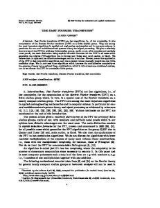
The structure of typical stages r k pipeline SDF architecture is depicted in Figure 1. It can be observed in the first row of Figure 1 that the output of one stage is connected to the input of the next stage. Within each stage, there is a sequence of hardware processing elements which can perform the computations defined by the operators presented in Section 2.2 as illustrated in the second and third rows of Figure 1. The hardware required to implement the computations demanded by each operator is discussed in (Cortés et al., 2009). It is important to note that the shuffling operators surrounding the butterfly operators can be merged in the single device with feedback typical of the SDF architecture. To illustrate this, in the fourth row of Figure 1 the implementation of radix 2k algorithms is presented. Each stage H( k,k,i) consists of k butterfly operators B, with their corresponding shuffling and unshuffling S and (S )−1 terms. The hardware that implements the arithmetic of the butterfly operators B is the same in all the stages of the FFT processor. The implementation of the butterfly depends on the value of r. The length of each of the delay lines used for the shuffling and unshuffling corresponding to the first butterfly of the first stage is N/r. The length of each of these delay lines is reduced by a factor of r from one butterfly to the next one as is shown in the fourth row of Figure 1. The number of delay commutator structures used for the shuffling and unshuffling around a butterfly unit is the same as the number of butterfly units. Operators M1, M2 and M3 mainly translate to complex multipliers (C.M.) and Look-Up Tables (LUTs) to store the twiddle factors (T.F.). A stage of the form H( k,k,i) has one twiddle factor multiplier operator M1. The number of twiddle factors stored in the LUT used to implement M1 is N for the first stage and it reduces by a factor of r k from one stage to the next. When N = r knk , no complex multiplier is needed to implement the twiddle factor multiplications given by M1( k( nk −1),k) of the last stage H( k,k,nk −1) , because M1( k( nk −1),k) = I N . The final processing given by terms of the form H( l,k,nk ) when N = r knk +l , with l = 0, does not actually have a operator M1; i.e.: M1( knk ,k) = I N . For k > 1, twiddle factor multiplier operators M2 appear. A stage H( b,k,i) has b/2 operators M2 when b is even and (b − 1)/2 when b is odd. The number of twiddle factors stored in the LUT used to implement M2 is always r2 . For k > 2, twiddle factor multiplier operators M3 appear. A stage H( b,k,i) has b/2 − 1 operators M3 when b is even and (b − 1)/2 when b is odd. The number of twiddle factors stored in the LUT used for the implementation of the first M3 within a stage H( b,k,i) is r b and it reduces by a factor of r2 from one M3 to the next one within the same stage. 2.5 Hardware resources of r k pipeline architectures

In (Cortés et al., 2009), the complexity of the r k algorithms in terms of area was analyzed. In this section, some of their conclusions are summarized. For a given N, the designer can vary the parameters r and k to achieve different implementations. These parameters influence the reordering operators and the arithmetic operators. The overall amount of memory words used for the delay lines due to the reordering operators depends neither on r nor k. In an SDF architecture, the amount of memory is N − 1 words.

Fast Fourier Transform Processors: Implementing FFT and IFFT Cores for Cores OFDM Communication Systems Fast Fourier Transform Processors: Implementing FFT and IFFT for OFDM Communication Systems 1) x nk−1

x2 x1 x0

H

(k,k,0)

H

(k,k,1)

H

Only if b>2

(k,k,i)

G

3)

S

B

G

S

(k,ki,1)

−1

G

M2

N/r ki+1

4)

(k,ki,n)

S

G

V

(k,ki,M)

B

S

−1

M3

N/r ki+2

B

H

(k,k,nk−1)

Only if b is even

2) (k,ki,0)

1199

B

S

S

−1

LUT

rk

S

−1

M1

N/r ki+1

B

LUT

B

M2

N/r ki+1

B

Fig. 1. Structure of typical stages of

S

(k,ki)

B LUT

LUT

pipeline SDF architectures

Therefore, the overall amount of memory words is fixed by the number of points of the FFT. N − 1 is the minimum amount of memory reported in the literature for a pipeline FFT architecture. Modifying the values of r or k does not increase the amount of memory words used for the reordering operators. Increasing the value of r for fixed values of N and k will reduce the number of butterflies and the overall number of complex multipliers. However, the butterflies become more complex. Regarding the number of twiddle factors, the number of twiddle factors due to M1 are reduced, while the number of twiddle factors due to M2 and M3 increase. For small values of k, there is a reduction of the overall number of twiddle factors; while for large values of k, there is an increase in the overall number of twiddle factors. Thus, the benefit of increasing the value of r depends on the value of k. If the values of N and r are fixed, the benefits of increasing k can be studied. The overall number of butterflies is logr N, and thus, increasing k does not increase either the number of butterflies or their area. Increasing the value of k reduces the number of complex multipliers due to M1. Once M2 and M3 appear in an architecture, the number of complex multipliers due to each one remains approximately constant. Thus, an important benefit of increasing the value of k is that it reduces the overall number of complex multipliers. When k increases, the number of twiddle factors due to M1 is reduced. For (logr N )/2 ≤ k < logr N, one single M1 with N twiddle factors appears. Finally, when k = logr N, M1 = I N and no hardware is needed to implement any M1. The number of twiddle factors due to M2 remains constant with k. The number of twiddle factors due to M3 increases with k. Adding the contributions of M1, M2 and M3, the overall number of twiddle factors first reduces with k and then it starts to increase. It can be concluded that an optimum value of k exists for each value of N and r. Usually this optimum value is near k = (logr N )/2. From the general expressions, the designer has to look for those values of r and k that result in an optimum single-path FFT pipeline architecture for a given application. This search can be easily performed thanks to the close link between the proposed matricial representation and implementation. No other notation allows such an exploration within the pipeline architectures.

120


10

3. Case study: WLAN IEEE 802.11a In this section, a case study is analyzed applying the proposed design space exploration in order to achieve the most efficient algorithm/architecture for an OFDM system. This design space exploration does not only analyze the hardware complexity of the algorithms as in (Cortés et al., 2009). Additionally, an implementation level analysis is carried out also taking into account the power consumption which is very important for wireless devices. The main objective of this design space exploration is to select the most efficient radix r k pipeline SDF FFT architecture for the OFDM application. An FFT for the WLAN IEEE 802.11a standard has been selected as the case study. In this case, the length of the FFT/IFFT is 64 points. According to (Cortés et al., 2009), the optimum value of k is near 3. Therefore, the following analysis concentrates on r = 22 , r = 23 and r = 24 algorithms in order to perform the implementation level analysis and to study the silicon area and power consumption results. The proposed design space exploration can be divided into four steps. At first, the OFDM system described by the standard is analyzed to extract the specifications. Once the OFDM specifications are known, the designer focuses on the system and on the FFT/IFFT specifications to determine the parameters needed for the FFT/IFFT design. The next step is the implementation level analysis of different FFT/IFFT algorithms and architectures in order to select the most efficient core for the WLAN system according to a given criterion. This step is composed of two main analysis: the Error Vector Magnitude (EVM) analysis in the transmitter and the Carrier-To-Noise Ratio (CNR) analysis in the receiver. After these analysis, the data bitwidth (dbw) and the twiddle factors bitwidth (tbw) are chosen so as not to degrade the system performance. Finally, the layout of the most efficient FFT/IFFT core for WLAN 802.11a in terms of area and power consumption is shown. 3.1 Study of the IEEE 802.11a standard

Table 2 shows the parameters specified in IEEE 802.11a standard for a WLAN system (IEE, 1999). Nc = 64 sub-carriers are used. Np = 4 sub-carriers are used as pilot tones to make the coherent detection more robust against frequency offsets and phase noise. These pilot tones are always in sub-carriers -21, -7, 7 and 21 and they are modulated in Binary Phase-Shift Keying (BPSK). Nd = 48 tones are employed as data sub-carriers and the rest of sub-carriers are zero. The length of the guard interval must be longer than the delay spread of the channel. R BW tsym EVM N f L p H/No (Mbps) (MHz) (μs) (dB) (dB) 16 54 20 4 -25 20 16 40

Nc Nd N p Ngi 64 48 4

Table 2. OFDM Parameters for a WLAN IEEE 802.11a system Considering an indoor environment, the necessary guard interval in a WLAN system is 0.8 μs. Therefore, the last Ngi = 16 data must be copied at the beginning of the OFDM symbol. The maximum data rate is R = 54 Mbps. Additionally, the bandwidth of the system is BW = 20 MHz. The standard also determines that the OFDM symbol period is tsym = 4μs. In IEEE 802.11a, data can be modulated in BPSK, Quadrature Phase-Shift Keying (QPSK), 16-Quadrature Amplitude Modulation (QAM) or 64-QAM.


The EVM is defined as: EVM =

( I − Io ) 2 + ( Q − Q o ) 2 ,

121 11

(23)

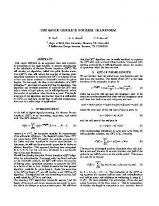
where I + jQ is the measured symbol and Io + jQo is the transmitted symbol. Figure 2 illustrates the computation of the EVM for a 16-QAM constellation. The IEEE 802.11a specifies I+jQ Io+jQo

EVM

Average Power Po=1

Fig. 2. EVM in the 16-QAM constellation a mean value Erms which has to be measured after transmitting N f = 20 frames of L p = 16 OFDM symbols with an average power Po , 16 (48+4) ∑ EVM ( i, j, k ) j =1 ∑ k =1 1 20 , (24) Erms = 20 i∑ (48 + 4)16 · Po =1 where EVM(i, j, k) is the magnitude of the error vector for the kth sub–carrier of the jth OFDM symbol of the i th frame. The EVM is the quality constraint that must not be degraded in the transmitter. The EVM value in Table 2 is the minimum EVM in a WLAN system when the system transmits data modulated in 64–QAM with the maximum data rate of 54 Mbps. The IEEE 802.11a standard specifies the spectral mask of the output signal in the transmitter. Figure 3 presents the spectral mask of the IEEE 802.11a transmitter output where this height is H/No = 40dB. The quality constraint selected for the receiver is the non–degradation of the CNR when the input signal to the receiver has the spectral mask specified by the standard. This is a first approach that produces an overconstrained core. EVM and H/No specifications are used to determine the allowed quantization error. 3.2 System analysis and FFT/IFFT specifications

The goal of this analysis is to determine the parameters of Table 3. Table 3 presents five important system specifications which influence significantly the design of the FFT/IFFT: the length of the FFT/IFFT N, the system clock frequency f clk, the value of Ktx in the transmitter, the value of K AGC and the CNR in the receiver. As the OFDM system supports 64 sub-carriers, the FFT core must be designed to perform 64-points FFT; i.e.: N = 64. As shown in Table 2, the OFDM symbol period (tsym ) in a WLAN system is equal to 4 μs. Following the analysis of (Velez, 2005), f clk = 60 MHz is selected, higher than the maximum data rate R and multiple of the BW.

122


12

Fig. 3. Spectral mask of a transmitter output N Length of the FFT/IFFT fclk System clock frequency Ktx Maximum gain to improve the DAC performance K AGC Maximum gain to improve the FFT performance CNRmax Maximum carrier–to–Noise Ratio Table 3. System specifications 3.2.1 k tx in the transmitter

In order to select Ktx , an analysis of the IFFT output data must be carried out for each OFDM system. For this analysis, the modulation where the data reach the highest values in the I and Q data must be used. In this analysis, Ktx is estimated by means of simulations. The transmission of the number of frames determined by the standard is simulated for different values of Ktx to calculate the EVM. Then, the largest Ktx that does not degrade the EVM can be selected. This way, the whole dynamic range of the Digital-to-Analog Converter (DAC) is exploited. Figure 4 shows the system model used to analyze the EVM degradation with the increase of the value of Ktx . The system model is composed of a floating–point IFFT in the transmitter and a floating–point FFT in the receiver. The effect of the clipping in the DAC is emulated by a limiter located after the multiplication by Ktx . This limiter is responsible for saturating the amplified IFFT output according to the integer bits of the data representation. Two integer bits are considered for both the input and output data in the IFFT, since the maximum value of the input data is 1.08 when the modulation is 64–QAM. In order to improve the dynamic range of the IFFT output, the data are amplified by a factor Ktx . A factor Ktx , which is a power of two, is preferred to simplify the hardware implementation. In (Velez, 2005), the overflow probability of the different types of modulations in WLAN is analyzed carrying out Monte Carlo simulations with 3 ≤ Ktx ≤ 10 . It is concluded that BPSK modulation is the most sensitive to the clipping at the DAC. (Velez, 2005) also concluded that the most suitable value

Fast Fourier Transform Processors: Implementing FFT and IFFT Cores for Cores OFDM Communication Systems Fast Fourier Transform Processors: Implementing FFT and IFFT for OFDM Communication Systems Floating−point IFFT

Floating−point FFT

K tx

123 13

1/K tx

EVM

Fig. 4. System model to study the effect of Ktx in EVM for Ktx is Ktx = 4 so as not to degrade the system performance. Additionally, Ktx = 4 is implemented as a simple shift in a real implementation. Figure 5 shows the effect of the factor Ktx on the EVM in the transmitter, that is, how the EVM is degraded by the clipping produced in the IFFT. If a factor Ktx = 8 were selected, the −15

EVM of the 64−point FFT, dB

−20 −25 −30 −35 −40 −45 −50 −55 −60 4

5

6

7

8

9

10

11

12

13

Ktx

Fig. 5. Analysis of the effect of the Ktx in EVM EVM value would not meet the standard specification. It can be observed that Ktx = 4 is a conservative decision, since the EVM specified by the standard for a BPSK modulation with a data rate of 9 Mbps is -8 dB, and the EVM obtained with Ktx = 4 is -61.95 dB. 3.2.2 k AGC and CNR max in the receiver

An Automatic Gain Control (AGC) module is a block found in many electronic devices. The AGC is commonly used to dynamically adjust the gain of the receiver amplifier to keep the received signal at the desired power level. In this analysis, the effect of the AGC is modeled as a gain K AGC. For the analysis, the value of K AGC that does not degrade the CNR, is selected. This value is determined by means of simulations. Figure 6 presents the system model to determine this factor K AGC. This model is composed by a floating-point IFFT at the transmitter and a floating-point FFT at the receiver. The channel is modeled as as an Additive White Gaussian Noise (AWGN) channel.

124


14

AWGN

xi

Floating−point IFFT

Xi

Yq

Y K AGC

Floating−point FFT

yq CNR

Yi

yi Floating−point FFT

K AGC

Fig. 6. System model to estimate the CNR for different values of K AGC Before applying the AWGN channel, the power of the output signal of the IFFT, Xi , is normalized to 1 dividing the signal by the factor λ, which is defined as Nd + Np . (25) λ= Nc2 In Figure 6, Y is the signal after applying the AWGN channel. At the receiver, this signal is multiplied by the gain K AGC and a limiter is applied. This limiter is responsible for limiting the amplified signal according to the number of integer bits of the data representation. Once the limiter is applied, Yq is the input of the floating-point FFT and yq is the output of the floating-point FFT. yi is the output of the floating-point FFT without noise and without applying the limiter. For the simulations, it is necessary to determine the variance of the noise to be applied to the transmitted signal so that the signal meets the spectral mask with the height H/No given by the standard. The Signal-To-Noise Ratio (SNR) of the transmitter output can be calculated from the height of the spectral mask H/No given by the standard. The power of the output signal of the transmitter can be written as, Po =

( Nd + Np ) · BW · ( H − No ) , Nc

(26)

where it is assumed that the power of the data sub-carriers is equal to the power of the pilot sub-carriers. The noise power is given by: Pn = No · BW.

(27)

Therefore, SNR =

( Nd + Np ) Po H =( − 1) · . Pn No Nc

(28)

Then, the variance σ2 of the noise in the channel is found to be, σ2 =

1

( NHo

− 1) ·

( Nd + Np ) Nc

.

(29)

In order to select the value of the factor K AGC, the CNR is used as a figure of merit. CNR is defined as, Pˆ (30) CNR = i , Pˆn


125 15

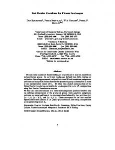
where Pî is the power of yi and Pˆn is the power of the difference between yi and yq . The gain K AGC is selected so that the CNR is not degraded. Factor K AGC fixes the power of the signal Yq ; i.e.: PYq . The figures to analyze the effect of K AGC on CNR plot the CNR versus PYq , which is a more representative value. The CNR is obtained by means of Monte Carlo simulations. This method allows the designer to estimate a measure of the performance of a communication system and the quality of the estimation itself (Sevillano, 2004). The looseness of our estimation in order to achieve a confidence interval equal to 0.95 is defined as, ˆ ) ˆ (CNR 2 · var (31) γ= ˆ CNR Therefore, it can be said that the probability of CNR belonging to the interval [(1 − ˆ (1 + γ )CNR ˆ ] is 0.95. The Monte Carlo simulations are stopped when γ < 10−2 . γ )CNR, It is assumed that the signal arrives with the maximum quality H/No = 40 dB. Therefore, applying (28), the SNR of the transmitted signal is of 39.09 dB. Figure 7 shows the (CNR)dB versus the power of the input signal of the FFT PYq . The signal works without degradation with PYq < −4 dB, which corresponds to K AGC = 6 in the simulations. For this value of K AGC, (CNRmax )dB is 39.1 dB. 40 39.5

CNR of the 64−point FFT, dB

39 38.5 38 37.5 37 36.5 36 35.5 35 −20

−18

−16

−14

−12

−10

−8

−6

−4

−2

0

Power of the FFT input signal, dB

Fig. 7. (CNR)dB vs the power of the input signal in the FFT (PYq ) 3.2.3 Summary of results

In this step, the length of the FFT N, the system clock frequency, f clk, the gain factor in the transmitter, Ktx , and the gain factor in the AGC, K AGC and the CNRmax have been estimated. Table 4 presents the necessary OFDM parameters for the next step.

126


16

Ngi

BW tsym EVM (dB) N f L p fclk N Ktx K AGC CNRmax (MHz) (μs) (MHz) (dB) 16 20 4 -25 20 16 60 64 4 6 39.1

Table 4. Specifications for the architecture selection for WLAN systems 3.3 Selection of algorithm/architectures

A high throughput FFT core is needed to fulfil the required specifications. Pipeline architectures are well suited to achieve small silicon area, high throughput, short processing time and reduced power consumption. Table 5 presents the hardware complexity of the candidate pipeline-SDF architectures. The pipeline-SDF radix 22 DIF architecture is composed Architec.

r Normal Constant ROM RAM adds mults. mults. (regs.) (regs.) /subs pipeline–SDF 22 8 0 80 192 28 pipeline–SDF 23 4 4 64 192 40 pipeline–SDF 24 4 4 64 192 35 Table 5. Hardware complexity of candidate FFT architectures working at 60 MHz for WLAN systems of six butterflies and two complex multipliers. The pipeline-SDF radix 23 DIF architecture is composed also of six butterflies, but one complex multiplier and two constants multipliers by one constant are used. The pipeline-SDF radix 24 DIF architecture is formed by six butterflies, one complex multiplier and one constant multiplier by two constants. Therefore, the three algorithms have the same number of multipliers taking into account normal and constant multipliers. The radix 23 and 24 DIF algorithms reduce ROM with respect to the radix 22 DIF one, but they add control logic. To sum up, at this point it is not clear which is the most efficient architecture for WLAN. Therefore, it is necessary to make an implementation level analysis. The hardware complexity of radix 22 , 23 and 24 DIF algorithms is compared to search the optimum design that meets the system specifications. The EVM constrains the word-length of the IFFT in the transmitter. The word-length in the receiver is constrained by the CNR. If the transmitter and the receiver are implemented in the same chip, the highest word-lengths must be chosen. The figures of merit to select the algorithm and architecture are the area and the power consumption estimated for an Application-Specific Integrated Circuit (ASIC) technology. Thus, this selection process can be stated as the problem of finding the FFT/IFFT processor which minimizes the AP cost function subjected to the constraints given by the specifications. The AP criterion trades off area and power consumption and can be used as a measure of the efficiency of the core. The area and power results presented in the following sections have been calculated for a TSMC 90 nm 6 ML technology with a clock frequency of 60 MHz working at 1.0V and a temperature of 25o C. The area results have been estimated multiplying the cell area by a factor of 2. 3.3.1 EVM analysis

In order to analyze the effect of the IFFT quantization error on the EVM during transmission, an ideal reception is considered. The system model is composed of a fixed-point IFFT at the


127 17

transmitter and a floating-point FFT at the receiver as can be seen in Figure 8(a). The EVM value is employed to select the values of dbw and tbw needed in the transmitter. An EVM margin of -10 dB is used in order to select a conservative word–length. Thus, a margin is left for other sources of error, such as the error produced by the analog processing. In order to FFT

IFFT FIXED−POINT

K tx

FLOATING−POINT

1/K tx

EVM

(a) EVM model AWGN

IFFT FLOATING−POINT

FFT K AGC

FIXED−POINT

CNR FFT K AGC

FLOATING−POINT

(b) CNR model

Fig. 8. System models to study the effect of quantization error on EVM and CNR obtain the EVM results in Figures 9 and 10 the transmission of N f = 20 frames of L p = 16 OFDM symbols modulated in 64-QAM has been simulated. The pipeline-SDF with the radix 22 , 23 and 24 DIF algorithms have been studied to find the most efficient implementation. For radix 23 and 24 algorithms, the bitwidth of the constant multiplier is assumed to be equal to the bitwidth of the normal multiplier. Figure 9 shows the EVM and the area results of the pipeline–SDF DIF 64–point FFT/IFFT core for different algorithms. In order to guarantee an EVM of at least -35 dB, the radix 22 algorithm requires a (dbw,tbw) of (12,8), whereas the radix 24 and 23 algorithms need (12,7). For the given EVM, the radix 24 algorithm achieves the smallest core with (dbw, tbw) = (12, 7). The EVM and the power results of the pipeline–SDF DIF 64–point FFT/IFFT core are presented in Figure 10. It can be observed that the radix 22 algorithm requires less power consumption for the same (dbw, tbw) than the rest of algorithms, whereas the radix 23 algorithms consume more than the others. Table 6 compares the area and the power consumption for the different algorithms to obtain an EVM of at least -35 dB. The power consumption in Table 6 has been normalized. (Kuo et al., Algorithm dbw tbw Area (mm2 ) 2 SDF r2 12 8 0.0993 SDF r23 12 7 0.0998 SDF r24 12 7 0.0960

Pnorm

AP

0.0211 0.00210 0.0233 0.00232 0.0222 0.00214

Table 6. AP comparison for WLAN system with EV M ≤ −35dB

128


18

0.13

(15,10) (15,10)

0.125

(15,10) (14,9)

Area of the FFT, mm2

(14,10) 0.12

(14,10)

(14,9)

(14,10) (14,9)

0.115

0.11

0.105 (12,8)

radix 22 0.1

(12,7)

3

(12,8)

radix 2

4

(12,7)

(12,8)

radix 2

(12,7) −55

−50

−45

−40

−35

−30

−25


Fig. 9. EVM and area of the pipeline–SDF DIF 64–point FFT/IFFT core 125 2

radix 2 3 radix 2 4 radix 2

124

Power of the FFT, mW

123 122

(12,9)

121

(12,7)

(12,9)

120

(12,7)

119 118 (12,9)

117 (12,8)

116 115 −44

−43

−42

−41

−40

−39

−38

−37

−36

−35

−34


Fig. 10. EVM and power of the pipeline–SDF DIF 64–point FFT/IFFT core 2003) proposes a normalization of the power consumption as, Pnorm =

P · 1000, 2 ·N· f VDD clk

(32)


129 19

where P is the power consumption with a voltage of VDD and working at f clk. By slightly modifying the expression given by (Kuo et al., 2003) as follows, Pnorm =

P · 109 . 2 · f VDD clk

(33)

The r22 algorithm needs larger bitwidths to achieve the target EVM. This extra bit in tbw increases the area needed. The r23 and r24 algorithms can achieve the required EVM with smaller tbw. The r24 algorithm with dbw = 12 and tbw = 7 achieves the most area–efficient implementation that fulfills the EVM specification. Nevertheless, the power consumption of the r24 algorithm is higher than the power consumption of r22 algorithm. In fact, the r22 algorithm is the most power–efficient design. In order to achieve a trade–off, the parameter AP = Area · Pnorm is employed since it takes into account the area and the power consumption. The AP parameter trades off the area and power consumption of the core and, thus, it measures the efficiency of the design. For WLAN transmitter, it can be observed in Table 6 that the most efficient cores are the ones using r22 and r24 algorithms. 3.3.2 CNR analysis

After the EVM analysis, the r23 algorithm is discarded. Therefore, the CNR analysis focuses on the r22 and r24 algorithms. At this point, the area and power results of the FFT/IFFT core for different bitwidth configurations are already known. Then, the CNR analysis is used to select the dbw and tbw which fulfills the CNR specification. In order to analyze the effect of the FFT quantization, the simulation model is formed by a floating–point IFFT at the transmitter and a fixed–point FFT at the receiver as is shown in Figure 8(b). First, only data are quantized. In this case, a figure of the CNR versus dbw can be used in order to select the dbw which does not degrade the CNR. Once dbw is selected, the twiddle factors are also quantized and a figure of the CNR versus tbw is shown in order to choose the tbw which does not degrade the CNR. This analysis is done for the candidates in order to determine the necessary dbw, tbw to comply with the CNR specification. As an example, figures of (CNR)dB versus dbw and tbw are given for two algorithms. Figure 11(a) shows the (CNR)dB obtained versus the dbw parameter. In this case, the twiddle factors are not quantized. From the figure, a data bitwidth of dbw = 15 is selected to avoid degrading the (CNR)dB for both radix 22 and radix 24 algorithms. Once the data bitwidth is chosen, the twiddle factors are quantized. Figure 11(b) presents the (CNR)dB versus tbw where dbw = 15. In this case, a twiddle factor bitwidth of tbw = 10 is selected for both radix 22 and radix 24 algorithms. It can be observed that increasing more tbw does not improve the performance of the core. Table 7 summarizes the (dbw, tbw) needed by the FFT to comply with the CNR requirement. Comparing the bitwidths needed by the IFFT in the transmitter to comply with the EVM and the ones needed by the FFT in the receiver to comply with the CNR, it can be said that the CNR is a much more restrictive specification. Therefore, the (dbw, tbw) selected for the FFT are the bitwidths used in the FFT/IFFT core. Table 7 presents the AP results of the FFT algorithms with the necessary bitwidths (dbw, tbw) to comply with the specifications. Taking into account the AP, the most efficient core for a WLAN system is the pipeline–SDF radix 22 DIF architecture.

130


20

40

39



38 36 34 32 30 28

38

37

36

35

34

26 24 10

radix 22 radix 24 11

12

13

14

15

16

dbw (bits)

17

18

19

radix 22 radix 24 33 7

8

9

10

11

tbw (bits)

12

13

14

15

(b) tbw (dbw = 15)

(a) dbw

Fig. 11. Selection of dbw and tbw of the pipeline–SDF DIF 64–point FFT/IFFT core for radix 22 and radix 24 algorithms Algorithm dbw tbw Area Pnorm AP (mm2 ) SDF r22 15 10 0.1284 0.0277 0.00356 SDF r24 15 10 0.1256 0.0287 0.00360 Table 7. AP comparison for WLAN system with (CNR)dB ≥ 38.32 dB To sum up, the parameters of the final implementation of the pipeline–SDF radix 22 DIF architecture are shown in Table 8. As mentioned before, the system clock frequency is 60 MHz. Working at this frequency, the processing time of the chosen core is 0.67 μs. The data format is 2.13, whereas the format of the twiddle factors is 1.9. The EVM is -51.92 dB and the (CNR)dB is 38.57 dB. The estimated silicon area of the pipeline–SDF radix 22 DIF FFT/IFFT core is 0.1284 mm2 and the power consumption estimation Pnorm is 0.0277. It can be observed that the EVM complies with the specification in Table 4, and the CNR is close to the CNRmax . N dbw tbw fclk t proc CNR EVM 64 15 10 60 MHz 0.67 μs 38.57 dB -51.92 dB Table 8. Core Parameters for the pipeline–SDF radix 22 DIF architecture 3.4 Layout of the FFT/IFFT core in an ASIC

Figure 12 shows the layout of the 64 complex–point FFT/IFFT fabricated in a 90 nm TSMC technology, 6–ML CMOS process. The core size is 0.1362 mm2 . In the previous section, the core area was estimated to be 0.1284 mm2 . It can be said that the area estimation is accurate enough. In order to present a comparison with the proposals found in the literature, the area of the cores is normalized as (B.M.Baas, 1999) using the equation: Anorm =

A , ( Ta /Tb )2

(34)


131 21

Fig. 12. Layout of the 64 complex–point FFT/IFFT fabricated in a 90 nm technology, 6–ML CMOS process. The core size is 0.370 × 0.368 mm2 . where Ta is the anchor of the transistor of the technology actually used, A is the occupied area for Ta and Tb is the technology for which the area is normalized. In order to assess the quality of the FFT/IFFT core, Table 9 makes a comparison with other 64 complex–point FFT/IFFT cores found in the literature. In Table 9, the area (Anorm ) and the power (Pnorm ) have been normalized to a 90 nm technology using (34) and (33). The AP parameter indicates that our core is the most efficient one for a WLAN application. In fact, the presented core requires the smallest normalized power (Pnorm). dbw tech. fclk

Anorm t proc Pnorm AP

(μm) (MHz) (mm2 ) (μs)

(Yu et al., 2011) 16 0.18 80 (Tsai et al., 2011) 14.8 0.09 394 Proposal 15 0.09 60

0.2209 – 0.0378 0.00835 0.102 – 0.091 0.00928 0.1362 0.67 0.0277 0.00377

Table 9. Comparison of fixed–point FFT processors for WLAN systems

4. Conclusions Many different FFT/IFFT algorithms and architectures have been proposed in the literature for OFDM systems as has been presented in Section 1. Additionally, the usual FFT notations do not facilitate to perform a general analysis for the FFT/IFFT algorithm and architecture selection. In Section 3, a design space exploration among different algorithms has been carried out. This search is hard to perform if general expressions are not available for the different algorithms in a unified way and if a mapping to the implementation can not be easily established. In this chapter, the matricial notation summarized in Section 2 is used as a tool to help the designer

132

22


in this search. The OFDM parameters obtained from the IEEE 802.11a standard analysis have been employed as constraints for the optimization problem. The AP parameter, which trades off area and power consumption, has been used as a measure of the efficiency of the core. Finally, a pipeline–SDF radix 22 DIF FFT/IFFT processor has been proposed, since it achieves the minimum of the AP cost function. To sum up, it can be concluded that there is no unique FFT/IFFT algorithm, architecture and implementation that is optimal for all OFDM systems. Therefore, it is recommended to perform a search across the algorithm, architecture and implementation dimensions for each OFDM system. The matricial notation is presented in this chapter as a unified and compact representation that can help the designer in this search. This search is feasible, and the FFT/IFFT cores implemented using this approach present a great efficiency.

5. References Bidet, E., Castelain, D., Joanblanq, C. & Senn, P. (1995). A Fast Single-Chip Implementation of 8192 Complex Point FFT, IEEE Journal of Solid State Circuits 30(3): 300–305. B.M.Baas (1999). A Low-Power, High Performance, 1024-point FFT Processor, IEEE Journal of Solid-State Circuits 34(3): 380–387. Bruun, G. (1978). z-Transform DFT Filters and FFTs, IEEE Transactions on Acoustics, Speech and Signal Processing 26(1): 56–63. Chang, Y.-S. & Park, S.-C. (2004). An Enhanced Memory Assignment Scheme for Memory-Based FFT Processor, IEEE Transactions Fundamentals E87-A(11): 3020–3024. Cooley, J. W. & Tukey, J. (1965). An Algorithm For Machine Calculation of Complex Fourier Series, Mathematics of Computation 19: 297–301. Cortés, A., Vélez, I. & Sevillano, J. F. (2009). Radix r k FFTs: Matricial Representation and SDC/SDF Pipeline Implementation, IEEE Transactions on Signal Processing 57(7): 2824–2839. Cortés, A., Vélez, I., Irizar, A. & Sevillano, J. F. (2007). Area efficient IFFT/FFT core for MB-OFDM UWB, Electronic Letters 43(11). ECM (2005). Standard ECMA-368, High rate ultra wideband PHY and MAC standard. Engels, M. (ed.) (2002). Wireless OFDM Systems. How to make them work?, Kluwer Academic. ETS (2004). Digital Video Broadcasting (DVB); Framing structure, channel coding and modulation for digital terrestrial television. Good, I. J. (1958). The Interaction Algorithm and Practical Fourier Analysis, Journal of the Royal Statistical Society 20(2): 361–372. He, S. & Torkelson, M. (1998). Designing Pipeline FFT Processor for OFDM (de)Modulation, URSI International Symposium on Signals, Systems, and Electronics 29: 257–262. IEE (1999). Part11: Wireless LAN Medium Access Control and Physical Layer specifications. High-speed Physical Layer in the 5 GHz Band. IEE (2003). Part 16: Air interface for fixed broadband wireless access systems amendment 2: Medium Access Control modifications and additional physical layer specifications for 2-11 GHz. Jiang, M., Yang, B., Fu, Y., Jiang, A. & an Wang, X. (2004). Design Of FFT processor with Low Power Complex Multiplier for OFDM-based High-speed Wireless Applications, International Symposium on Communications and Information Technologies pp. 639–641. Jung, Y., Yoon, H. & Kim, J. (2005). New Efficient FFT Algorithm and Pipeline Implementation Results for OFDM/DMT Applications, IEEE Transactions on Consumer Electronics 49(1): 14–20.


133 23

Kuo, J.-C., Wen, C.-H., Lin, C.-H. & Wu, A.-Y. (2003). VLSI Design of a Variable-Length FFT/IFFT Processor for OFDM-Based Communication Systems, EURASIP Journal on Applied Signal Processing pp. 1306–1316. Lee, H.-Y. & Park, I.-C. (2007). Balanced Binary-Tree Decomposition for Area-Efficient Pipelined FFT Processing, IEEE Transactions on Circuits and Systems-I 54(4): 889–900. Lee, J., Lee, H., Cho, S.-I. & Choi, S.-S. (2006). A High-speed, Low-complexity Radix-2 FFT Processor for MB-OFDM UWB Systems, IEEE International Symposium on Circuits and Systems pp. 4719–4722. Lenart, T. & Owal, V. (2006). Architectures for Dynamic Data Scaling in 2/4/8k Pipeline FFT Cores, IEEE Transactions on Very Large Scale Integration (VLSI) Systems 14(11): 1286–1290. Lin, H.-L., Lin, H., Chen, Y.-C. & Chang, R. C. (2004). A Novel Pipelined Fast Fourier Transform Architecture for Double Rate OFDM Systems, IEEE Workshop on Signal Processing Systems Design and Implementation pp. 7–11. Lin, Y.-W., Liu, H.-Y. & Lee, C.-Y. (2004). A Dynamic Scaling FFT Processor for DVB-T Applications, IEEE Journal of Solid-State Circuits 39(1): 2005–2013. Lin, Y.-W., Liu, H.-Y. & Lee, C.-Y. (2005). A 1-GS/s FFT/IFFT Processor for UWB Applications, IEEE Journal of Solid-State Circuits 40(8): 1726–1735. Liu, L., Ren, J., Wang, X. & Ye, F. (2007). Design of Low-Power, 1GS/s Throughput FFT Processor for MIMO-OFDM UWB Communication System, IEEE International Symposium on Circuits and Systems pp. 2594–2597. Maharatna, K., Grass, E. & Jagdhold, U. (2004). A 64-Point Fourier Transform Chip for High-Speed Wireless LAN Application Using OFDM, IEEE Journal of Solid-State Circuits 39(3): 484–492. Nee, R. V. & Prasad, R. (2000). OFDM for Wireless Multimedia Communications, Artech House. Pease, M. (1968). An Adaptation of the Fast Fourier Transform for Parallel Processing, Journal of the Association of Computing Machines 15(2): 252–264. Rader, C. M. (1968a). A Linear Filtering Approach to the Computation of the Discrete Fourier Transform, Northeast Electronics Research and Engineering Meeting Record 10: 218–219. Rader, C. M. (1968b). Discrete Fourier transforms when the Number of Data Samples is Prime, ˝ Proceedings of the IEEE 56: 1107U–1108. Rudagi, J. M., Lobo, R., Patil, P. & Biraj, N. (2010). An Efficient 64-point Pipelined FFT Engine, 2010 International Conference on Advances in Recent Technologies in Communication and Computing pp. 204–208. Saberinia, E. (2006). Implementation of a Multi-band Pulsed-OFDM Transceiver, Journal of VLSI Signal Processing 43: 73–88. Serrá, M., Martí, P. & Carrabina, J. (2004). IFFT/FFT core architecture with an Identical Stage Structure for Wireless LAN Communications, IEEE 5th Workshop on Signal Processing Advances in Wireless Communications pp. 606–610. ˜ de un Demodulador QPSK para Sistemas de Radiodifusión Digital por Sevillano, J. F. (2004). Diseno Satélite, PhD thesis, Campus tecnológico de la Universidad de Navarra. Sloate, H. (1974). Matrix Representation for Sorting and the FFT, IEEE Transactions on Circuits and Systems CAS-21(1): 109–116. Thomas, L. H. (1963). Using a Computer to Solve Problems in Physics, Applications of Digital Computers .

134

24


Tsai, P.-Y., Chen, C.-W. & Huang, M.-Y. (2011). Automatic IP Generation of FFT/IFFT Processors with Word-length Optimization for MIMO-OFDM Systems, EURASIP Journal on Advances in Signal Processing 2011(ID-136319). Tsai, T. H., Peng, C. C. & Chen, T.-M. (2006). Design of a FFT/IFFT Soft IP Generator using on OFDM Communication System, WSEAS Transactions on Circuits and Systems 5(8): 1173–1180. Turrillas, M., Cortés, A., Sevillano, J. F., Vélez, I., Oria, C., Irizar, A. & Baena, V. (2010). Comparison of area–efficient FFT algorithms for DVB-T2 receivers, Electronic Letters 46(15). Velez, I. (2005). Metodología de Diseño de Sistemas Digitales para Telecomunicaciones basada en C/C++: Aplicación a WLAN 802.11a, PhD thesis, Campus tecnológico de la Universidad de Navarra. Wang, C. C., Huang, J. M. & Cheng, H. C. (2005). A 2K/8K mode Small-Area FFT Processor for OFDM Demodulation of DVB-T Receivers, IEEE Transactions on Consumer Electronics pp. 28–32. Winograd, S. (1978). On Computing the Discrete Fourier Transform, Mathematics of Computation 32: 175–199. World DAB Forum (n.d.). http://www.worlddab.org/. Yu, C., Yen, M.-H. & Hsiung, P.-A. (2011). A Low-Power 64-point Pipeline FFT/IFFT Processor for OFDM Applications, IEEE Transactions on Consumer Electronics 57(1): 40–45.