C.S. Patlak, R.G. Blasberg, and J.D. Fenstermacher. Graphical evaluation of blood- to-brain transfer constants from multiple-time uptake data. J. Cereb.
Fast GPU Fitting of Kinetic Models for Dynamic PET Benjamin R. Smith, Ghassan Hamarneh and Ahmed Saad Medical Image Analysis Lab, Simon Fraser University, Canada
Abstract. We address the problem of quickly and accurately fitting compartmental models to large numbers of measurements, with application to dynamic positron emission tomograph imaging. An analytic method of calculating the model output function is developed, and compared to the numerical method used by COMKAT [5], the de facto kinetic modeling software. A performance increase of over 130� is demonstrated. Also, we describe a GPU implementation of the Levenberg–Marquardt optimization algorithm, using the developed analytic formulation, and apply it to compartmental model fitting. A fitting rate of 74,906 TAC/s was achieved, allowing a dPET volume to be fit in 13.8 seconds. In comparison, COMKAT would take 21.5 days to perform the same fitting.
1
Introduction
Molecular Imaging: Dynamic Positron Emission Tomography (dPET) is a functional imaging modality that allows minimally-invasive in-vivo observation of tissue metabolism. dPET operates via the tracer principle: a carefully chosen tracer molecule is injected into a subject, at levels which do not disrupt the system of interest. The tracer is radioactively tagged, such that the interaction of the tracer with tissues can be observed via the spatial and temporal concentration of observed decay events. A dPET system produces a 3D+time image: at each spatial location in the field of view, a time series of tracer concentration measurements is reconstructed. Each time series measurement (at a particular pixel) is known as a time activity curve (TAC). Models (e.g. exponential) of the underlying tissue-tracer interactions can be fit to each TAC, and the model parameters can describe important underlying characteristics of the tissue of interest (e.g. binding potential). In oncology, for example, cancerous tissue tends to exhibit a higher glucose metabolic rate (GMR) than normal tissue, which can be computed by fitting a model of glucose metabolism to observed activity. Tracer Models: Typically, tracer-tissue interactions are modeled using compartmental models, which describe the state and time–varying concentration of an injected tracer as a set of discrete compartments. Connections between compartments represent allowed flow and flow rates between compartments. One commonly used tracer molecule is 18 F-fluorodeoxyglucose (FDG). A two tissue compartmental model for FDG is shown in Fig. 1. The tracer enters the
2
Fig. 1. Standard compartmental model of FDG. FDG is introduced into the plasma via injection, and reaches tissues of interest where it is metabolized, transitioning between free and bound compartments.
plasma via an injection, and reaches tissues of interest. The states of the tracer: extra–cellular and metabolized, can be described as the tracer being in a “free” or “bound” compartment, respectively. FDG is a glucose analog, and is metabolized by cells in proportion to their energy demand. After metabolism, FDG is unable to leave the cell until it undergoes radio–active decay. The distribution of FDG throughout tissue is therefore characteristic of that tissue’s energy demand. Kinetic Modeling: The rate of exchange of FDG between plasma, unbound, and bound compartments can be specified as a set of rate constants: K1 , k2 , k3 , k4 . Mathematically, the model is expressed as a set of ordinary differential equations: dCF dt dCB dt
� K1 CP � k2 CF � k3 CF
k4 CB
� λCF ,
� k3 CF � k4 CB � λCF .
(1)
The concentration of tracer as a function of time, for plasma, free, and bound compartments is written as CP ptq, CF ptq, and CB ptq, respectively. The decay constant λ specifies the rate of decay of the radioactive tracer. Although radioactive decay is sometimes omitted from the model in favor of correcting the observed data, Glatting et. al [2] demonstrated that its inclusion in the model is more accurate and reduces variability in parameter estimates. The solution of (1) describes the concentrations of each compartment at any given time. However, TACs measured using a dPET imaging system are actually the sum of concentrations over all compartments. This sum of concentrations is referred to as the output equation, Optq. As shown by Gunn et. al [3], the output function can be expressed as a sum of exponentials convolved by the input function, If , which describes the injected tracer concentration as a function of time. The output function for a general C �compartment model (e.g. the 2– compartmental model of Fig. 1) is: O ptq �
C ¸
�
i 1
�
Ci ptq � If
�
C ¸
�
ϕi e�θi t
��
ptq .
(2)
i 1
The constants θi and ϕi are directly related to the rate constants ki of (1). The convolution operator, , is an important part of this paper, and its evaluation will be discussed further in Section 2. While (2) describes the concentrations as a continuous function of time, in practice, dPET images are reconstructed discretely as 3D volumetric frames over a fixed time interval. The observed concen-
3
tration, T AC ptq, at a given pixel and frame is the average concentration during that frame. The average concentration of a frame starting at ts and ending at te can be described by the normalized integral M pts , te q over rts , te s as: T AC ptq � M pts , te q �
1
te � tb
»te
O ptq dt.
(3)
ts
This equation is a mathematical model for the observed TAC in a dPET scan, and it is of practical interest to fit this model and obtain the unknown parameters. However, fitting observations to the model equation (3) can be time intensive: it is nonlinear due to the presence of exponential terms, and there are typically a large number of TACs measured in an image. A typical dPET volume has dimensions of 128 � 128 � 64, which can potentially mean fitting 1,048,576 models to observed TACs. One alternative is to fit only a representative subset of TAC observations (e.g: averages of TACs derived from regions of interest). Another alternative is to use a simplified model, based on assumptions about the underlying tissue or tracer [7]. These alternatives require assumptions or conceal features of the underlying data. Ideally, a fast and accurate method is needed to fit entire TAC volumes. This is the goal of our work. Overview of CUDA and the GPU: If computation can be efficiently divided into multiple subproblems, it can potentially be computed more quickly in parallel. Of particular interest to this work, is the application of a graphics processing unit (GPU) for fast, massively parallel fitting of kinetic models that are prohibitively expensive to do sequentially. Over the last decade, high performance GPUs have become available to the public for affordable prices. GPUs are powerful processing resources, which have begun to eclipse the abilities of a standard computer processor. The realization that GPUs could be exploited for general purpose computing has led to their use in many non-graphical tasks, such as clustering, data classification, scientific computing and general mathematics [6]. Previously, use of the GPU for general purpose computing has required specific knowledge of graphics rendering, and an ability to translate the problem of interest into an equivalent rendering problem. More recently, the introduction of software application programming interfaces, such as CUDA (nVidia Co., Santa Clara, CA), has abstracted away many of the GPU details, allowing a programmer to develop significantly faster code, and deal with a minimal set of GPU specifics. However, not all computations are suited for the GPU. Typically, GPUs are single-instruction multiple-data (SIMD) devices. That is, they are very efficient at performing the same algorithmic steps, in parallel, on large sets of data. For example, nVidia’s GeForce GTX 285 GPU (used in this work) has 30 multi-processors, each capable of running 1024 concurrent threads. For a SIMD compatible algorithm, 30 � 1024 instances of a problem could potentially be solved in approximately the time it takes to solve a single instance on the CPU!
4
Levenberg–Marquardt for Nonlinear Fitting: The Levenberg–Marquardt algorithm [4] is a popular iterative method for nonlinear optimization, often used for fitting general non–linear models. Of particular interest, it can be used to fit compartmental models to observed dPET data. The algorithm is essentially a hybrid of the Gauss–Newton (GN) method and gradient descent (GD). The GN method is guaranteed to converge quickly if the current parameter estimate is close to a local optima, whereas GD will always converge to a local optima, but may do so slowly. The trade–off between the two algorithms is controlled by a damping parameter, which is changed iteratively according to the local curvature of the fitting function. Given an initial guess of the unknown model parameters, the algorithm makes GD-like steps when it is far from a minima (high curvature), and takes GN steps when close to the minima (low curvature). Contributions: We address the problem of quickly and accurately fitting compartmental models to large numbers of observations, with application to dPET imaging. First, the difference in performance between analytic and numeric methods of calculating the output function and its derivatives is examined. We demonstrate that analytic methods provide superior accuracy and computational performance: offering a speed-up of over 130� that of the equivalent numerical fitting. Second, a GPU implementation of the Levenberg-Marquardt nonlinear optimization algorithm [4] was developed, and applied to fit compartmental models in parallel using the analytic formulation. The increase in performance was examined with increasing parallelism, and the time required to fit a typical TAC volume was estimated. At the maximum level of parallelism permitted by the hardware used, a fitting rate of 74,906 TAC/s, was achieved, allowing a volume of 128 � 128 � 64 TAC to be fit in 13.8 seconds: a performance increase of 131,415�. COMKAT, the de facto software for kinetic fitting, would take 21.5 days to perform an equivalent fitting.
2
Method
Analytic Kinetic Model Fitting: While the COMKAT kinetic modeling software is popular and easy to use, it is slow: taking several seconds to fit a kinetic model to a single TAC. This slow performance has made it difficult to perform large numbers of fittings, or incorporate kinetic information into iterative algorithms. Therefore, only a few such methods are found in the literature [9]. A close examination of COMKAT reveals its reliance on a general numeric solver to compute fittings. This solver permits COMKAT to fit many different models, however it also requires a numeric convolution of a finely sampled input function, resulting from (2). Not only is this computationally expensive, but is a potential source of error. However, Feng et. al [1] have previously shown that the input function can be modeled by a combination of exponential terms, for particular tracers (e.g: FDG). Using an analytic input function for If , the convolution operation in (2) can be evaluated analytically, and the numerical convolution and
5
temporal sampling of the input function can be avoided entirely. Additionally, an analytic input function permits the calculation of an analytic Jacobian for use in fitting TAC. This increases the fitting accuracy (compared to a numerical approximation) and the convergence speed of the fitting process. Derivation of Analytic Output Function and Jacobian: Below, we derive a closed form analytic expression for (2), free of the convolution operator, in order to increase speed and accuracy of model fitting. This is accomplished by using an analytic form of the input function If . The derivation can be generalized for any If which is approximated by a sum of exponential terms of the form ak e� λk t , but we will focus specifically on the input function used by the COMKAT tool, a linear summation of 4 exponential terms (4). Note that the effect of the radioactive decay constant introduced in (1), λ, is implicitly incorporated into each constant λi . If
4 ¸
�
ai e� λi t
�
(4)
i 1
Expanding the convolution operator in the output function (2), substituting the input function (4) and performing a series of algebraic manipulations, the output function can be expressed analytically: O ptq �
»t � ¸ 4
�
τ 0
�
ai e� λi τ
i 1
��
C ¸
�
ϕi e� θi pt�τ q
�
i 1
�
N ¸ 4 ¸
� �
i 1j 1
�
� aj θi e� λj t � e� φi t . φi � λj
(5) Further, the analytic Jacobian is computed by taking derivatives with respect to the model parameters θi and ϕi . To preserve numerical accuracy of floating point operations, terms which have similar magnitude are grouped together. The final analytic expressions of (3) and its derivatives are given by (6), (7) and (8):
M pts , te q �
1
te � tb
N ¸ 4 ¸
�
� �
i 1j 1
aj θi φi � λ j
�
e� φi te
� e�φ t � e�λ t � e�λ t φ λ i s
j e
i
j s
,
j
(6)
BM � 1 ¸4 � aj � e�φ t � e�φ t � e�λ t � e�λ t Bθk te � tb j�1 pφk � λj q φk λj k e
k s
j e
j s
�
� �λ t BM � θk ¸4 aj e � e�λ t � e�φ t � e�φ t Bφk te � tb j�1 pφk � λj q2 λj φk � �φ t
� � φ t � φ t � φ t � ts e e �e . � φ a�j λ te e φk φ2k k j j e
k e
k s
j s
k e
k e
k s
k s
,
(7)
(8)
6
Parallel Levenberg–Marquardt: As discussed above, the speed of model fitting can be further increased by performing the fitting as a parallel calculation. The key is to note that each TAC can be fit independently of the others. Each thread of execution will fit a TAC in a straightforward, serial manner, running an independent instance of the Levenberg–Marquardt algorithm. The chief complication is that this requires the algorithm to execute as a SIMD algorithm: all threads must simultaneously execute the same calculation on different data. Therefore the parallel fitting will take as long as the longest serial fitting. Threads which complete early will perform no work until the remainder complete. This is a current limitation of parallel GPU programming in general.
3
Validation and Results
In order to evaluate the performance of the developed analytic formulation, its accuracy and speed was compared to the numeric method used by COMKAT. Synthetic TAC fitting problems were created that were increasingly difficult to fit, by corrupting observations with noise and initializing the algorithms increasingly further from the correct answer. In addition, the performance of the developed parallel fitting method was measured, and the time required to fit a typical dPET volume using the proposed method was estimated. Numeric vs. Analytic Fitting: Two experiments were performed to compare the speed and accuracy of compartmental model fitting using analytic and numeric formulations. The analytic output function and Jacobian of the FDG model (6), (7) and (8), were implemented in MATLAB 7.0.1 (Mathworks, Natick, MA) and used as input to the “lsqnonlin” fitting function. To ensure comparability, the Levenberg-Marquardt algorithm was specifically selected from available optimizers. Results were compared to the COMKAT 3.2 fitting tool that also makes use of the “lsqnonlin” implementation, but employs numerical methods. Computations were performed using an Intel Core i7 920 64 bit CPU, 2.67 GHz, with 6 gigabytes of RAM. Synthetic TAC data was generated using the analytic output function (3) and kinetic parameters chosen randomly from a valid range of kinetic parameters [8], defined as: K1 P r0.037, 0.134s, k2 P r0.112, 0.3s, k3 P r0.031, 0.188s, k4 P r0.003, 0.017s. Non-uniform frame sizes (12 � 10 s, 10 � 30 s, 10 � 2 min, 10 � 5 min, 4 � 10 min) were selected to more finely sample frames with more dynamic activity. The input function was defined with parameters ai � t650, 146, 105, 21u and λi � t6.7, 0.25, 0.03, 0.0001u. First, the effect of initialization on the optimization process was studied. For each synthetic TAC, an initialization was created by adding a perturbation to the kinetic parameters used to generate that TAC. Perturbations were drawn from a uniform distribution of increasing fractions of the valid parameter ranges tested: p0.1, 0.23, 0.36, 0.5q. At each level, 20 TACs were created and fit. The effect of noise on TAC fitting was also studied. Normally distributed noise was added to each TAC, with increasing standard deviation. Four noise levels, σ � t0.0, 3.33, 6.67, 10.0u pmol/ml, were tested. A typical TAC, corrupted
7
Fig. 2. A typical TAC, used to evaluate the effect of noise on model fitting algorithms. corrupted by increasing levels of noise.
by each noise level, is shown in Fig. 2. Initial parameters were created by drawing perturbations from a uniform distribution of up to 0.25 of the valid parameter ranges. These perturbations were selected as reasonable based on the first experiment. At each noise level, 20 TACs were created, noise added, and fitted. In each experiment, TACs were fit to compartmental models using 4 Levenberg– Marquardt variants: (i) COMKAT, (ii) an analytical output function with numerically estimated Jacobian (ANALYTIC), (iii) an analytic output and Jacobian function (ANALYTIC+JAC), and (iv) the CUDA implementation of Levenberg-Marquardt with analytic output and Jacobian (CUDA), running serially. Execution time was measured, and the speed multiplier compared to COMKAT was computed, and plotted in Fig. 3. Note that for these experiments, the CUDA timings are provided for reference only. The CUDA implementation uses CUDA 3.0 and C++ code, and is not directly comparable to MATLAB implementations. The absolute percentage error for each kinetic parameter was calculated. Error in GMR, a common clinical PET parameter, was also computed and reported. These results are shown in Fig. 4 for perturbed initialization, and Fig. 5 for varying levels of noise.
Fig. 3. Comparison of TAC fitting speed (in TAC/s), as a ratio to COMKAT’s speed, for different fitting methods with varying degrees of perturbed initialization (left) and varying levels of additive noise (right). All tested methods were significantly faster, on average, than COMKAT. Under perturbed initialization ANALYTIC, ANALYTIC+JAC and serial CUDA were approximately 90�, 130�, and 62� faster, respectively. Under increasing noise, ANALYTIC, ANALYTIC+JAC, and serial CUDA were approximately 132�, 172�, and 83� faster, respectively. Note that COMKAT is not directly comparable to CUDA due to implementation details.
8
Fig. 4. Comparison of error fitting kinetic parameters, with varying degrees of perturbed initialization. The proposed methods are more accurate than COMKAT. The CUDA implementation is slightly less accurate than the corresponding MATLAB implementation, but still significantly more accurate than COMKAT.
It was expected that all tested methods would have comparable error, but that analytic methods would be faster than COMKAT. In the perturbed initialization experiment, ANALYTIC, ANALYTIC+JAC, and CUDA are approximately 94�, 132.5�, and 61.6� faster than COMKAT (Fig. 3, and this effect was relatively independent of the degree of perturbation. Similarly, in the noisy TAC fitting experiment, ANALYTIC, ANALYTIC+JAC, and CUDA are approximately 132.6�, 171.7� and 82.8� faster than COMKAT, and the speed-up trended slightly upward with respect to noise level, as COMKAT slowed with noise. This confirmed the expectation that the analytic forms are faster than the numeric implementation. Note that the CUDA implementation is executing serially in these experiments, and the slower performance relative to the other analytic methods is due to differences in implementation. The errors of the fit parameters, as a percentage of their true value, were plotted in Fig. 4 and Fig. 5 for the perturbation and noise experiments respectively. In the perturbed initialization experiment, the analytic methods were consistently more accurate than COMKAT, which demonstrated that not only are the former methods faster, but they are slightly more accurate. It is interesting to note the significantly higher error fitting k4 . The magnitude of this parameter is quite small, and the effect of slight errors is magnified when considering the % error. In the noise experiment, error for all test methods is comparable, and increases with noise. Again, COMKAT demonstrates significantly higher error for k4 , which is more sensitive to small errors. Parallel Analytic Fitting: To determine the performance improvement of increased parallelism on fitting, and to study the expected time required to fit large numbers of TACs, a further experiment was performed using the CUDA
9
Fig. 5. Comparison of error fitting kinetic parameters, with varying levels of added noise. ANALYTIC+JAC and CUDA demonstrated less error than COMKAT during fitting under various noise levels, though ANALYTIC demonstrated higher error.
implementation of Levenberg–Marquardt fitting. As before, synthetic TAC were generated. Initialization was created by randomly perturbing correct parameter values by up to 0.25 of the valid ranges defined. Normally distributed noise with σ � 5.0 pmol/ml was added to each TAC. Five sets of 10,000 TACs were generated with different noise and initialization realizations. The CUDA implementation was then used to fit each generated TAC. The number of TAC to fit in parallel was varied from 1 (serial execution) to 10,000. Execution time was recorded at each level of parallelism. Results are reported in Fig. 6. The predicted behavior was that increasing parallelism would result in significant speed-up. Subject to the limits of the hardware, as parallelism increased by a factor of 10, the speed of TAC fitting should increase by a factor of 10. As shown in Fig. 6, this was precisely what was observed: TAC fitting speed increased by a factor of 10 for each increase in parallelism by factor 10, up until 1,000. At this level, the limit of parallelism due to memory requirements of the GPU was reached. The logarithmic plot of TAC fit over time, in Fig. 6, illustrates this relationship. Given the observed TAC fitting speed, the time required to fit a dPET volume of 128 � 128 � 63 can be estimated as approximately 13.8 seconds. This can be loosely compared to the time required for COMKAT, at 0.57 TAC/s, of nearly 21.5 days. This is a performance increase of approximately 131,415�.
4
Conclusions
We have demonstrated that fitting large numbers of TAC, typical of the number in a patient volume, can be accomplished accurately and quickly using commodity hardware. Through the use of the analytic form of the input function,
10 Parallelism Speed (TAC/s) 1 45 10 450 100 4,505.6 1,000 33,758.4 10,000 74,906.4 Fig. 6. Comparison of time-to-fit TAC for increasing levels of parallelism in CUDA implementation. Smaller slope values indicate improved performance. For each 10� increase in parallelism, time-to-fit decreased by 10�, up until 1, 000 TAC.
it is possible to avoid expensive numerical convolution and calculate accurate Jacobians for faster, more accurate fitting. Further, we have demonstrated that by exploiting the independence of each fitting, it is possible to create a massively parallel implementation of the Levenberg–Marquardt algorithm using the CUDA framework. This enables typical patient volumes to be fit in under 13.8 seconds, compared to many days using conventional software. These techniques have potential application for iterative methods for PET that incorporate kinetic models, such as kinetically regularized dPET reconstruction or image segmentation. While our experiments are performed on synthetic data, the TAC observed in dPET are understood to be well modeled by the compartmental models used to generate them, and we expect our results to generalize well to real data.
References 1. D. Feng, S.C. Huang, and X. Wang. Models for computer simulation of input functions for tracer kinetic modeling with PET. Int. Bio. Comp., 32:95–110, 1993. 2. G. Glatting and S.N. Reske. Treatment of radioactive decay in pharmacokinetic modeling: inflence on parameter estimation in cardiac 13N-PET. Med. Phys., 26(4):616–621, 1999. 3. R.N. Gunn, S.R. Gunn, and V.J. Cunningham. PET compartmental models. J. Cereb. Blood Flow and Metab., 21(6):635–652, 2001. 4. K. Levenberg. A method for the solution of certain non–linear problems in least squares. Q. Appl. Math., 2(2):164–168, Jul. 1944. 5. R. Muzic and S. Cornelius. COMKAT: compartment model kinetic analysis tool. J. Nucl. Med., 42(4):636–645, 2001. 6. J.D. et. al Owens. A survey of general–purpose computation on graphics hardware. Comp. Graphics Forum, 26(1):80–113, 2007. 7. C.S. Patlak, R.G. Blasberg, and J.D. Fenstermacher. Graphical evaluation of bloodto-brain transfer constants from multiple-time uptake data. J. Cereb. Blood Flow and Metab., 3:1–7, 1983. 8. M. et. al Piert. Diminished glucose transport and phosphorylation in Alzheimer’s disease determined by dynamic FDG-PET. J. Nucl. Med., 27:201–208, 1996. 9. A. Saad, B. Smith, G. Hamarneh, and T. M¨ oller. Simultaneous segmentation, kinetic parameter estimation, and uncertainty visualization of dynamic PET images. In MICCAI (2), pages 726–733, 2007.