mand increases to query graphs over a large data graph. In this paper, we study a graph pattern matching problem that is to retrieve all patterns in a large graph, ...
Fast Graph Pattern Matching Jiefeng Cheng1 1
Jeffrey Xu Yu1
Bolin Ding1
Philip S. Yu2
Haixun Wang2
The Chinese University of Hong Kong, Hong Kong, China, {jfcheng,yu,blding}@se.cuhk.edu.hk 2 T. J. Watson Research Center, IBM, USA, {psyu,haixun}@us.ibm.com
Abstract
lationships in social networks [3], finding research collaboration patterns, and finding research paper citation connection in archived bibliography datasets. The graph pattern matching problem can be considered as an extension of finding twig-patterns (tree patterns) over XML tree. However, the existing techniques for processing twig-patterns over XML tree [8, 14] cannot be effectively applied to handle graph pattern matching over a large directed graph. It is because a graph does not have the nice property such that every two nodes are connected along a unique path. In a large data graph, a node, vi , can reach another node vj , while the same vi is possibly reachable from vj .
Due to rapid growth of the Internet technology and new scientific/technological advances, the number of applications that model data as graphs increases, because graphs have high expressive power to model complicated structures. The dominance of graphs in real-world applications asks for new graph data management so that users can access graph data effectively and efficiently. In this paper, we study a graph pattern matching problem over a large data graph. The problem is to find all patterns in a large data graph that match a user-given graph pattern. We propose a new two-step R-join (reachability join) algorithm with filter step and fetch step based on a cluster-based join-index with graph codes. We consider the filter step as an R-semijoin, and propose a new optimization approach by interleaving R-joins with R-semijoins. We conducted extensive performance studies, and confirm the efficiency of our proposed new approaches.
Contributions of this paper: We propose processing graph pattern matching as a sequence of R-join (reachability join) upon a graph database which stores a data graph in tables. We propose a new two-step R-join algorithm with a filter step and fetch step, based on a new cluster-based join-index with graph codes for reachability checking. Furthermore, we consider the first filter step as an R-semijoin, and propose a new optimization approach to optimize a sequence of R-joins/R-semijoins. We conducted extensive performance studies, and confirm the efficiency of our proposed new approaches.
1 Introduction A graph provides great expressive power to describe and understand the complex relationships among data objects. With the rapid growth of World-Wide-Web, new data archiving and analyzing techniques, there exists a huge volume of data available in public, which is graph structured in nature including hypertext data, semi-structured data [1]. RDF also allows users to explicitly describe semantic resource in graphs [7]. In [27], Shasha et al. highlighted algorithms and applications for tree and graph searching including graph/subgraph matching in data graphs. The demand increases to query graphs over a large data graph. In this paper, we study a graph pattern matching problem that is to retrieve all patterns in a large graph, GD , that match a user-given graph pattern, Gq , based on reachability. As an example, based on business relationships, a graph pattern can be specified as to find Supplier, Retailer, Wholeseller, and Bank such that Supplier directly or indirectly supplies products to Retailer and Whole-seller, and all of them receive services from the same Bank directly or indirectly over a large data graph which can be obtained from the Web. Similar needs also stem from finding web-services connection patterns in WWW, finding re-
Organization: We give the problem statement in Section 2. In Section 3. we discuss our R-join/R-semijoin approach. We propose a new two-step R-join algorithm (filter/fetch) based on which an R-semijoin is introduced. We propose a new R-join/R-semijoin order selection approach in Section 4. In Section 5, two existing approaches are discussed. We conducted extensive performance studies using large datasets and report our findings in Section 6. Related work is given in Section 7. Section 8 concludes the paper.
2 Problem Statement In this section, we give our problem statement following the discussions on data graph and graph pattern. A data graph is a directed node-labeled graph GD = (V, E, Σ, φ). Here, V is a set of nodes; E is a set of edges (ordered pairs); Σ is a set of node labels, and φ is a mapping function which assigns each node, vi ∈ V , a label lj ∈ Σ. We use label(vi ) to denote the label of node vi . Given a label X ∈ Σ, the extent of X, denoted as ext(X), is the set 1
a0
b0 b2 c1 d2
b3 d3
b4 c2
e1 e2 e3 e4 e5 e6
b1 c0
b5
d1
d0
c3
e0 d5 e7
d4
A
b6
called 2-hop reachability labeling [17]. A 2-hop reachability labeling over graph GD assigns every node v ∈ V a label L(v) = (Lin (v), Lout (v)), where Lin (v), Lout (v) ⊆ V , and u ; v is true if and only if Lout (u) ∩ Lin (v) 6= ∅. A 2-hop reachability labeling for GD is derived from a 2-hop cover of GD . In brief, given GD , the 2-hop cover minimizes a set of S(Uw , w, Vw ), as a set cover problem. Here, w ∈ V (GD ) is called a center, and Uw , Vw ⊆ V (GD ). S(Uw , w, Vw ) implies that, for every node, u ∈ Uw and v ∈ Vw , u ; w and w ; v, and therefore u ; v. Consider Figure 1, an example is S(Lin , w, Lout ) = S({b3 , b4 }, c2 , {e0 }). Here, c2 is the center. It indicates: b3 ; c2 , b4 ; c2 , c2 ; e0 , b3 ; e0 , and b4 ; e0 . There are several implementations to find such 2-hop cover for GD [23, 24, 15]. The 2-hop cover update problem is addressed in [24]. We proposed a fast algorithm to compute 2-hop cover [15]. Let H = {Sw1 , Sw2 , · · · } be the set of 2-hop cover computed, where Swi = S(Uwi , wi , Vwi ) and all wi are centers. The 2-hop reachability labeling for a node v is L(v) = (Lin (v), Lout (v)). Here, Lin (v) is a set of centers wi where v appears in Vwi , and Lout (v) is a set of centers wi where v appears in Uwi . Based on the 2-hop reachability labeling, we store graph GD into a database, GDB , by taking a node-oriented representation. There are |Σ| tables for GD . A table TX , for a label X ∈ Σ, has three columns named X, Xin and Xout . For each node xi ∈ ext(X) (⊆ V (GD )), there is a tuple in table TX . The X column keeps the node identifier xi . The Xin and Xout columns keep its Lin (xi ) and Lout (xi ), respectively. We assume that the X column is the primary key of the table, because a node in GD is uniquely identified with a node identifier. We call TX a base table if it is the table for a label X ∈ Σ.
B C
D
(a)
E (b)
Figure 1. Data Graph (a) & Graph Pattern (b) of all nodes in GD whose labels are the same X. A simple data graph, GD , is shown in Figure 1 (a). There are 5 labels, Σ = {A, B, C, D, E}. In Figure 1 (a), a node in an extent ext(X) is represented as xi where x is a small letter of X with a unique number i to distinguish it from others in ext(X). For example, ext(C) = {c0 , c1 , c2 , c3 }. In the following, we use V (G) and E(G) to denote the set of nodes and the set of edges in graph G. A graph pattern is a connected directed node-labeled graph Gq = (Vq , Eq ), where Vq is a subset of labels (Σ), and Eq is a set of edges (ordered pairs) between two nodes in Vq . An edge (X, Y ) ∈ E(Gq ) represents a reachability condition, denoted X֒→Y , for X, Y ∈ Vq . A reachability condition, X֒→Y , requests two nodes vi and vj in GD , for label(vi ) = X and label(vj ) = Y , vj is reachable from vi , denoted vi ; vj . A match in GD matches graph pattern Gq if it satisfies all the reachability conditions conjunctively specified in Gq . Note: X֒→Y and Y ֒→Z implies X֒→Z. A result that matches a n-node graph pattern Gq is a nary tuple, hv1 , v2 , · · · , vn i. A graph pattern, Gq , is shown in Figure 1 (b). There are five labeled nodes: A, B, C, D, and E, and there are four edges (reachability conditions), A֒→C, B֒→C, C֒→D and D֒→E, which conjunctively specify a graph pattern to be found. Consider the data graph GD in Figure 1 (a). There is a match in GD that matches the graph pattern, Gq , shown in Figure 1 (b), ha0 , b0 , c1 , d2 , e1 i. In detail, a0 ; c1 satisfies A֒→C, b0 ; c1 satisfies B֒→C, c1 ; d2 satisfies C֒→D, and d2 ; e1 satisfies D֒→E. Note: c1 is reachable from both a0 and b0 and can reach d2 , and a0 ; c1 and c1 ; d2 imply a0 ; d2 . Graph Matching Problem: A graph matching problem is to find all matches in an arbitrary large directed data graph GD that match all the reachability conditions conjunctively specified in a graph pattern, Gq .
Example 3.1: A graph database GDB for GD (Figure 1) is shown in Figure 2 (a). There are five tables: TA (A, Ain , Aout ), TB (B, Bin , Bout ), TC (C, Cin , Cout ), TD (D, Din , Dout ), and TE (E, Ein , Eout ). For a tuple xi in table TX , we make 2-hop reachability labeling compact by removing xi from its Xin and Xout columns. Hence, Lin (xi ) = Xin ∪{xi } and Lout (xi ) = Xout ∪{xi }. Below, we call Lin (xi ) and Lout (xi ) graph codes for xi , denoted in(xi ) and out(xi ). The reachability, xi ; yi , returns true, if out(xi ) ∩ in(yj ) 6= ∅. 2
3 A New Join-Based Approach
3.1 R-Join
In this paper, given a graph pattern Gq , we propose graph matching as a sequence of joins, where each reachability condition, X֒→Y ∈ E(Gq ), is a join, called R-join (for reachability join). Such an R-join is possible based on a graph labeling
Given two base tables in GDB , a reachability condition, X֒→Y , in a graph pattern Gq , can be processed as an R-join between two tables, TX and TY . TR ← TX 1 TY X֒→Y
2
(1)
Here, an R-join implies that, for every xi ∈ ext(X) and yj ∈ ext(Y ), xi ; yj holds, if the reachability condition, X֒→Y , is evaluated to be true using the graph codes. A pair, hxi , yj i, appears in the temporal table TR , if xi ; yj is true (out(xi ) ∩ in(yj ) 6= ∅). Consider TB 1 TE , hb0 , e7 i appears in the result, be-
A a0 B b0 b1 b2 b3 b4 b5 b6 C c0 c1 c2 c3
B֒→E
cause out(b0 ) = {b0 , c1 }, in(e7 ) = {c1 , e7 }, and out(b0 ) ∩ in(e7 ) 6= ∅. In general, an R-join over any two tables, TR and TS , with a reachability condition, X֒→Y , can be specified. Note: X (Y ) is the column in the base table TX (TY ), that may appear in a temporal table because of a previous R-join. Here, TR and TS can be either a base or temporal table. X֒→Y
(3)
TX 1 TR
(4)
X֒→Y
a0 F
b6 c0 c2 d0 d1 e0
Dout ∅ ∅ {c1 } {c1 } ∅ ∅ Eout ∅ ∅ . . . ∅
(D,E) (C,E) (D,C) (D,D)
{c1 } {c1 , c2 } {c1 } {c1 }
F
b6 b1
B+ Tree
c0 T
b6
F
c0
c1 T
c0 d0 d1
F
a0 b0 b2 c1 d2 d3
c2 T
c1 d2 d3 e1
F
b3 b4 c2
c3 T
c2 e0
F
c3 b6 b5 e0
T
c3 d4 d5
e7
(c) A Cluster-Based R-Join-Index
Figure 2. A Graph Database for GD (Figure 1) Swi = S(Uwi , wi , Vwi ) and all wi are centers. It is a B+ tree in which its non-leaf blocks are used for finding a given center wi . In the leaf nodes, for each center wi , its Uwi and Vwi , denoted F-cluster and T-cluster, are maintained. We further divide wi ’s F-cluster and T-cluster into labeled F-subclusters/T-subclusters where every node, xi , in an Xlabeled F-subcluster can reach every node yj in a Y -labeled T-subcluster, via wi . It is important to note that, in our cluster-based R-join index, we keep node identifiers (tuple identifiers) instead of pointers to tuples in base tables. With this arrangement, we can answer some R-join without accessing base tables. If there is a need to access a base table, we use the primary index built on the base table. Together with the cluster-based R-join index, we design a W -table in which, an entry W (X, Y ) is a set of centers. A center wi will be included in W (X, Y ), if wi has a nonempty X-labeled F-subcluster and a non-empty Y -labeled T-subcluster. It helps to find the centers, wi , in the clusterbased R-join index, that have an X-labeled F-subcluster and a Y -labeled T-subcluster.
X֒→Y
X֒→Y
(TR 1 TS ) 1 TT ≡ TR 1 (TS W ֒→Z
b6 T
a0 b2
...
a0
where TR can be a base/temporal table. The following holds for R-joins. TR 1 TS ≡ TS 1 TR (Commutative), X֒→Y
{a0 , c1 , c3 } {c1 , c2 , c3 } {c0 , c1 , c3 } {a0 , c1 , c3 } {c0 , c1 , c2 , c3 }
(A,C) (B,C) (C,D) (A,D) (C,C)
root
As a special case, a self-R-join is a join that can be processed as a selection, TR 1 TR (5)
X֒→Y
Din {a0 , c0 } {a0 , c0 } {c1 } {c1 } {c3 } {c3 } Ein {a0 , c2 } {c1 } . . . {c1 }
(b) W-table
Therefore, a graph pattern, Gq , can be specified as a sequence of R-joins followed by a projection to project the columns for every label X ∈ V (Gq ). In this paper, we concentrate ourselves on query processing and optimization over multi R-joins, and focus on discussions of finding an optimal query plan that is represented as a left-deep tree [29] in which an R-join is either between two base tables or between a temporal table and a base table. As shown in Eq. (3) and Eq. (4) below, TX and TY represent base tables, and TR represents either a base or a temporal table. X֒→Y
D d0 d1 d2 d3 d4 d5 E e0 e1 . . . e7
(a) Five Base Tables {a0 } {a0 , c1 } {c1 , c2 } {c1 , c3 } {b0 , b6 }
(A,B) (A,E) (B,E) (B,D) (B,B)
(2)
TR 1 TY
Aout {c1 , c3 } Bout {c1 } {c3 , b6 } {c1 } {c2 } {c2 } {c3 } {c3 } Cout ∅ ∅ ∅ ∅
...
TRS ← TR 1 TS
Ain ∅ Bin ∅ ∅ {a0 , b0 } {a0 } {a0 } {a0 } {a0 } Cin {a0 } ∅ {a0 } ∅
1 TT ) (AssoW ֒→Z suppose TR keeps tuples
X֒→Y
ciative). Given a table TR and that satisfy two reachability conditions, A֒→B and B֒→D. Then the tuples in TR satisfy A֒→D (Transitive).
3.2 A Cluster-Based R-Join Index Like a θ-join, an R-join needs to check the reachability condition X֒→Y at run time, which incurs high cost. We propose a join-index approach, which is to index all tuples xi and yj that can join between two tables, TX and TY . With such a join-index, an R-join can be efficiently implemented as to fetch the results. We build a cluster-based R-join index for a data graph GD based on the 2-hop cover computed, H = {Sw1 , Sw2 , · · · }, using our fast algorithm in [15], where
Example 3.2: The GDB for GD (Figure 1) is shown in Figure 2. Figure 2 (a) shows the five base tables, Figure 2 (c) shows the clustered-based R-join index, and Figure 2 (b) 3
them into the answer set R (line 6). The output of an Rjoin between two base tables is a set of pairs hxi , yj i for xi ; yj . It is important to note that there is no need to access base tables because all the nodes are maintained in the cluster-based R-join index to answer the R-join. In order to process multi R-joins, we need a way to process an R-join between a temporal table and a base table. In general, a temporal table TR has columns which are all the labels that are involved in the previous R-joins. Its tuples satisfy all the previous R-joins. We propose a new two-step R-join algorithm in Algorithm 2, called HPSJ+. It processes TR 1 TY , where TR is a temporal table that has an X col-
Algorithm 1 HPSJ (TX , TY , X֒→Y ) 1: 2: 3: 4: 5: 6: 7: 8:
C ← W(X, Y ) using the W -table; R ← ∅; for each wk ∈ C do Xk ← getF(wk , X) using the cluster-based R-join index; Yk ← getT(wk , Y ) using the cluster-based R-join index; R ← R ∪ (Xk × Yk ); end for return R;
Algorithm 2 HPSJ+ (TR , TY , X֒→Y ) 1: TW ← Filter(TR , X֒→Y ); 2: TRS ← Fetch(TW , X֒→Y ); 3: return TRS ; 4: Procedure Filter(TR , X֒→Y ) 5: TW ← ∅; 6: for each tuple, ri , in TR do 7: Xi ← getCenters(xi , X, Y ) where xi is in X column in ri ; 8: insert (ri , Xi ) into TW if Xi 6= ∅; 9: end for 10: return TW ; 11: 12: 13: 14: 15: 16: 17: 18:
X֒→Y
umn, and TY is a base table that has a Y column. Below, we discuss the HPSJ+ algorithm in detail. A join algorithm can be implemented in a similar manner like Algorithm 2 to process (TR 1 TX ), where TR is a temporal table that has X֒→Y
a Y column, and TX is a base table that has an X column. The HPSJ+ algorithm takes three inputs, a temporal table TR , a base table TY , and an R-join condition X֒→Y . In HPSJ+, first, it calls a procedure Filter(TR , X֒→Y ) to filter TR tuples that cannot be possibly joined with TY using W -table, and stores them into TW (line 1). Second, it calls a procedure Fetch(TW , X֒→Y ) to fetch the R-join results using the cluster-based R-join index. We do not need to access the base table TY , because the needed nodes are stored in the cluster-based R-join index. The details of the two procedures are given below. In Filter(TR , X֒→Y ), first, it initializes TW to be empty (line 5). Second, in a for-loop, it processes every tuple ri in TR iteratively (line 6-9). In every iteration, it obtains a set of centers, Xi , for xi in the X column in ri , where every center wk in Xi must have some yj ∈ TY in its T-cluster (line 7). It is done using getCenters(xi , Y ) below.
Procedure Fetch(TW , X֒→Y ) TRS ← ∅; for each (ri , Xi ) ∈ TW do for each wk ∈ Xi do Yi ← getT(wk , Y ) using the cluster-based R-join index; TRS ← TRS ∪ ({ri } × Yi ); end for end for
shows its W -table. The cluster-based R-join index (Figure 2 (c)) has six centers, a0 , b6 , c0 , c1 , c2 , and c3 . The W -table (Figure 2 (b)) tells where R-join can find its centers in the cluster-based R-join index. Consider TA 1 TB . The entry W (A, B) keeps {a0 }, A֒→B
which suggests that the answers can only be found in the clusters at the center a0 . As shown in Figure 2 (c), the center a0 has an A-labeled F-subcluster {a0 }, and a B-labeled Tsubcluster {b2 , b3 , b4 , b5 , b6 }. The answer is the Cartesian product between these two labeled subclusters. 2
getCenters(xi , X, Y ) = out(xi ) ∩ W(X, Y )
(6)
As shown in Eq. (6), out(xi ) is a set of centers wk that xi can reach. It needs to access the base table TX using the primary index. We use a working cache to cache those pairs of (xi , out(xi )), in our implementation to reduce the access cost for later reuse. W(X, Y ) is the set of all centers, wk , such that some X-labeled nodes can reach wk and some Y labeled nodes can be reached by wk . The intersection of the two sets is the set of all centers such that xi must be able to reach some yj ∈ ext(Y ). If Xi 6= ∅, it implies that xi must be able to reach some yj (line 6), and therefore the pair of (ri , Xi ) is inserted into TW (line 8). Otherwise, it can be pruned. In Fetch(TW , X֒→Y ), it initializes TRS as empty (line 12). For each pair of (ri , Xi ) ∈ TW , it obtains its Y -labeled T-subcluster, using getT(wk , Y ), stores them in Yi (line 15), conducts Cartesian product between {ri } and Yi , and puts them into TRS (line 16). As an example, consider (TB 1 TC ) 1 TD
3.3 R-Join Algorithms We first outline an R-join algorithm (Algorithm 1) between two tables discussed in [16], and then discuss a new two-step R-join algorithm (Algorithm 2) between a temporal table and a base table proposed in this paper. The HPSJ algorithm (Algorithm 1) processes an R-join between two base tables, TX 1 TY . First, it gets all cenX֒→Y
ters, wk , that have a non-empty X-labeled F-subcluster and a non-empty Y -labeled T-subcluster, using the W -table, and maintains it in C (line 1). Second, for each center wk ∈ C, it conducts three things. (1) It obtains its Xlabeled F-subcluster, using getF(wk , X), and stores them in Xk (line 4). (2) It obtains its Y -labeled T-subcluster, using getT(wk , Y ), and stores them in Yk (line 5). Both (1) and (2) are done using the cluster-based R-join index. (3) it conducts Cartesian product between Xk and Yk , and saves
B֒→C
4
C֒→D
Consider ((TB 1 TC ) 1 TD ) 1 TE . Suppose we
to access GDB (Figure 2). First, Algorithm 1, processes TB 1 TC and results in a tem-
B֒→C
becomes (TBC 1 TD ) 1 TE . Then,
C֒→D C֒→E e TD ) 1 TE (TBC 1 TD ) 1 TE = ((TBC ⋉ TD ) ⊲⊳ C֒→D
C֒→E
C֒→D
C֒→E
C֒→D
C֒→E
C֒→E
C֒→D
C֒→E
C֒→D
C֒→E
The conditions used in the two R-semijoins are C֒→D and C֒→E. Both access C in table TBC . If we process the two R-semijoins one followed by another, we need to ′ scan the table TBC , get another temporal table TBC , and ′ then process the second R-semijoin against TBC . Instead, we can process the two R-semijoins together, which only requests to scan TBC once. The Filter cost can also be shared. It can be done by simply modifying Filter. Due to space limit, we omit the details.
3.4 R-Semijoins Reconsider HPSJ+ (TR , TY , X֒→Y ) for an R-join between a temporal table TR and a base table TY . It can be simply rewritten as Fetch(Filter(TR , X֒→Y ), X֒→Y ) as given in Algorithm 2. Recall: the Filter prunes those TR tuples that cannot join any TY using the W -table. The cost of pruning TR tuples is small for the following reasons. First, W -table can be stored on disk with a B+ -tree, and accessed by a pair of labels, (X, Y ), as a key. Second, the frequently used labels are small in size and the centers maintained in W (X, Y ) can be maintained in memory. Third, the number of centers in a W (X, Y ) on average is small. Fourth, the cost of getCenters (Eq. (6)) is small with caching and sharing (Remark 3.1). We consider Filter () as an R-semijoin Eq. (7). (7) TR ⋉ TY = πTR (TR 1 TY )
Remark 3.1: (R-Semijoins Processing) In general, a sequence of R-semijoins, (((TR ⋉ TX1 ) · · · ) ⋉ TXk ) can be Ck
C1
processed together by one-scan of the temporal table TR under the following conditions. First, it is a sequence of R-semijoins, and there is no any R-join in the sequence. Second, let Ci be a reachability condition, Xi ֒→Yi . Either all Xi or all Yi are the same for a label appearing in TR . 2
4 Order Selection In this section, we focus ourselves on R-join/R-semijoin order selection. We maintain the join sizes and the processing costs for all R-joins between two base tables in a graph database. In order to find an optimized left-deep tree query plan, we estimate the cost for a self-R-join (Eq. (5)), which can be done as a selection, and a join between a temporal table and a base table. We adopt the similar techniques to estimate joins/semijoins used in relational database systems. Note: our approaches is not independent on a cost model. The cost parameters are listed in Table 1.
X֒→Y
Here, label X appears in the temporal table TR and label Y appears in the base table TY . X֒→Y
C֒→D
e TD ) ⊲⊳ e TE = (((TBC ⋉ TD ) ⋉ TE ) ⊲⊳
C֒→D
X֒→Y
C֒→D
e TD ) ⋉ TE ) ⊲⊳ e TE = (((TBC ⋉ TD ) ⊲⊳
tuples (b3 , c2 ) and (b4 , c2 ), in TBC are pruned because out(c2 ) = {c2 } and W(C, D) = {c0 , c1 , c3 }, and the intersection is empty (Eq. (6)). Fetch returns the final results, which are {(b0 , c1 , d2 ), (b0 , c1 , d3 ), (b2 , c1 , d2 ), (b2 , c1 , d3 ), (b5 , c3 , d4 ), (b5 , c3 , d5 ), (b6 , c3 , d4 ), (b6 , c3 , d5 )}.
TR ⋉ TX = πTR (TR 1 TX )
C֒→E
B֒→C
poral table, TBC = {(b0 , c1 ), (b2 , c1 ), (b3 , c2 ), (b4 , c2 ), (b5 , c3 ), (b6 , c3 )}. Note: only the clusters maintained in the three centers W (B, C) = {c1 , c2 , c3 } need to be used (Refer to Figure 2 (b)). Next, Algorithm 2 processes TBC 1 TD . In the Filter, the two
X֒→Y
C֒→D
process TB 1 TC first, and maintain the result in TBC . It
B֒→C
(8)
Eq. (8) shows a similar case where label Y appears in the temporal table TR and label X appears in the base table TX . The R-semijoin discussed in this work is different from the semijoin discussed in distributed database systems which is used to reduce the dominate data transmission cost over the network at the expense of the disk I/O access cost. In our problem, there is no such network cost involved. A unique feature of our R-semijoin is that it is the first of the two steps in an R-join algorithm. In other words, it must process R-semijoin to complete R-join. Below, we use e denote Fetch(). ⋉ denote Filter() as an R-semijoin and ⊲⊳ Then, we have
|TX 1 TY | |TRS |
=
|TR | ·
|TRS |
=
|TR | ·
|TRS |
=
|TR | ·
X֒→Y
|TX | · |TY | |TX 1 TY | X֒→Y
|TX | |TX 1 TY | X֒→Y
|TY |
(10) (11) (12)
(9)
Eq. (10) estimates the size of a self-R-join (Eq. (5)), with condition X֒→Y , using the join selectivity for the R-join TX 1 TY between two base tables TX and TY (the sec-
It is worth noting that the cost for both sides of Eq. (9) are almost the same.
ond term on the right side). Eq. (11) and Eq. (12) estimate the join size for R-joins (Eq. (3) and Eq. (4)), respectively.
TR 1 TS X֒→Y
e TS ≡ (TR ⋉ TS ) ⊲⊳ X֒→Y
X֒→Y
X֒→Y
5
Symbol
Meanings
IOH IOF T IOXY
Search cost over the B+ -tree (BH ). Disk access cost for one page scan in the FH file. Average cost of using R-join index to find an X-labeled node x, such that x ∈ πX (TX ⋉ TY ) .
F IOXY
Average cost of using the R-join index to find a Y -labeled node y, such that y ∈ πY (TY ⋉ TX ).
is the estimated cost for evaluating the subquery GS being considered under the current status S. Its search space is bounded by O(2m ), where m is the number of edges in Gq .
X֒→Y
4.2 Interleave R-Joins with R-Semijoins
X֒→Y
Recall: 1 is equivalent to ⋉ (Filter()) followed by e (Fetch()). In this section, we propose a new dy⊲⊳ namic programming solution by interleaving R-joins with e R-semijoins, or in precise, by interleaving ⋉ and ⊲⊳. Here, we define a status, S, as a four element tuple, (E, L, B in , B out ). A minimum-cost plan P is associated e being deterwith a status which is a sequence of ⋉ and ⊲⊳ mined. We explain the four elements below. First, E is the set of edges (R-joins) in E(Gq ), that are already included in P associated with S. Note: an edge X֒→Y is said to be ine are both included cluded in E, if its corresponding ⋉ and ⊲⊳ in P. Second, L is the set of labels that appear in the lefthand side of an R-semijoin or any side of an R-join. Third, B in (B out ) is a set of labels, where each label X ∈ B in (∈ B out ) indicates that the graph code in (out) in the base e TX is cached and can be used to process any remaining ⊲⊳, that has not been considered in the plan P yet. It is ime portant to note that E is only related to 1 (both ⋉ and ⊲⊳), and the other two elements, B in and B out , are only related e There are three possible moves: a move by an addito ⊲⊳. e (Fetch), and tional ⋉ (Filter), a move by an additional ⊲⊳ a move by an additional R-join (1), We call them, Filtermove, Fetch-move, and R-join-move, respectively. Note: the R-join-move is designed to use HPSJ (Algorithm 1) to R-join the initial two base tables, and the other two moves are design to HPSJ+ (Algorithm 2).
Table 1. I/O Cost Parameters The second terms on the right in Eq. (11) and Eq. (12) estimate a ratio if it joins with an additional base table. The cost for self-R-join (Eq. (10)) is 2 · (IOH + IOF ) · |TR |, because it needs to access the graph codes for checking xi ; yj . The cost for R-join between a temporal table and a base table (Eq. (11) and Eq. (12)) is (IOH + IOF ) · T |TR | + IOXY · |TRS |. Here, the two terms are for Filter() and Fetch(), the first term is the cost to retrieve graph codes using getCenters (Algorithm 2 line 7), and the second term is multiplication of the number of total nodes retrieved on R-join index by the average cost for finding out each node on R-join index. The size estimation of R-semijoins can be done in a similar way. We omit it due to space limit. In the following, we concentrate ourselves on R-join/R-semijoin order selection.
4.1 R-Join Order Selection Join processing has been widely studied [20, 22, 18, 19, 9, 21, 29]. We use dynamic programming, as one of the main techniques, for join order selection. In this section, we discuss R-join order selection, and do not consider Rsemijoins. We will discuss R-join/R-semijoin order selection in next subsection. The two basic components considered in dynamic programming are statuses and moves.
Filter-move: It corresponds to the addition of a new label, X, into B in (or B out ) due to the inclusion of ⋉
• A status, Si , specifies a subquery, Gsi (⊆ Gq ), as an intermediate stage in generating a query plan. The intermediate result by evaluating the query graph Gs is represented as R(Gsi ). • A move from one status (subquery Gsi ) to another status (subquery Gsj ) considers an additional edge (Rjoin) in Gsj that does not appear in Gsi . The next status is determined based on a cost function which results in the minimal cost, in comparison with all possible moves. The process of moving from one status to another results in a left-deep tree.
X֒→Y
(or (or
⋉ ), where X must be in L, if L = 6 ∅, and
Y ֒→X
e ⊲⊳
X֒→Y
e ) has not been included yet. When moving to ⊲⊳
Y ֒→X in
(E, B ∪ {X}, B out) (or to (E, B in , B out ∪ {X})), it does not only append TR ⋉ TS (or TR ⋉ TS ), but also all X֒→Y
Y ֒→X
other ⋉ on X to maximize the cost sharing (Remark 3.1). All possible R-semijoins can be considered. Fetch-move: Consider the status S = (E, L, B in , B out ), all e be a unfinunfinished Fetch are in E(Gq ) − E. Let ⊲⊳ X֒→Y
ished Fetch, a move from S to S ′ = (E ∪ {(X֒→Y )}, B in , e , if its ⋉ has been included. B out ) appends P ⊲⊳
The goal is to find the sequence of moves from the initial status S0 toward the final status Sf with the minimum cost, cost(Sf ), among all the possible sequences of moves. The determination of moves is based on a cost function. Such a cost function is associated with a status S, denoted cost(S), which is the minimal accumulated estimated cost needed to move from the initial status S0 to the current status S. Such accumulated cost of a sequence of moves from S0 to S
X֒→Y
Note:
⋉
X֒→Y
X֒→Y
is included if either X is in B out , or Y is in
B in . As a special case, if both X ∈ B out and Y ∈ B in , 1 is a self R-join, which can be processed in this status X֒→Y
together.
R-join-move: Consider the status S = (E, L, B in , B out ), 6
B in Bout (iii)
S0 S1
(i) (ii)
......
5
C E C E (i) (ii) in (iii) Bout B C
E
S2 10
A
(i)
A
E
E
B
A
C D E
C
C
C
D
D
E
E
C
C
B
C
C D E
A
(iii) B in C Bout C
(i)
~
A
C
E
C
D
D
E
(ii)
B C D E
A D
D
29.56
(iii) B in Bout
(i)
C
C
(ii)
......
B
A
C
E
E
D
C
C
C
D
D
E
(ii)
C
(i)
......
C
C
(iii) B in Bout C
27.22
S7 B
~ A
D E
B
B in C Bout
A
A
C
C
C
D
D
E
B
A
D
C
A
S9
S8
C
S6 A
...... 23.24 ......(ii) 23.24
~
C
C
B
D
E
18.89
C
A CA C (i) (ii) in (iii) Bout B 18
C
B
(iii) B in C (ii) Bout 15.33 S5
S4 A C D D 15.33 EC E (i) (ii) in (i) (iii) Bout B C
C D E
C
(L, B in , B out ), which determine the number of statuses. Note that B in ∪ B out ⊆ L. Thus regarding a node vq ∈ V (Gq ), there are 5 possible cases: 1) vq 6∈ L; 2) vq ∈ L, vq 6∈ B in , vq 6∈ B out ; 3) vq ∈ L, vq ∈ B in , vq 6∈ B out ; 4) vq ∈ L, vq 6∈ B in , vq ∈ B out ; 5) vq ∈ L, vq ∈ B in , vq ∈ B out . There are in total 5n combinations. Therefore, the total number of statuses is n · 5n . The space complexity is O(n · 5n ). There are m possible moves from each status, hence the total time complexity is O(mn · 5n ). The time complexity becomes O(mn · 3n ), if B in and B out is replaced by a single set as B in ∪ B out , where our previous discussions of moves fit as well with the implication that the Xin and Xout columns of a base table TX are accessed with the other each time. As a closely related issue of this problem, Wu et al. in [29] studied a tree-structured query graph for accessing XML data which is tree structured. The time complexity of their algorithm is O(n2 · 2n ). In this paper, we study graph pattern matching over a large data graph. The time complexity of our solution is reasonable comparing the time complexity of O(n2 · 2n ) for accessing a large XML tree.
S3 A
C
10
C
B
A
C E (i)
C
......
B
6
E
D
D
E
(ii)
C
C
C
A
B
A
(iii) B in C Bout C
......
Figure 3. Order Selection all unfinished Fetch are in E(Gq )− E. Let 1 be a unfinX֒→Y
ished R-join, a move from S to S ′ = (E ∪ {(X֒→Y )}, B in , B out ) appends 1 into P. Note: this R-join-move is only
5 Two Existing Approaches
X֒→Y
allowed to move from the initial status S0 to another status. Consider the query graph, Gq , in Figure 1. Figure 3 illustrates several moves for finding the minimum-cost Rjoin/R-semijoin plan from S0 . A status is shown in a block in Figure 3 with the following attributes: (i) subgraph of Gq being considered, (ii) a plan in the form of left-deep tree for (i), and (iii) B in and B out . Those subgraphs in a dotcircled in (i) shows L. The edges appear in a dot-circled is E. Initially, the start status S0 = (∅, ∅, ∅, ∅). From S0 , there are 4 possible R-join-moves, because there are n = 4 edges in Figure 1, plus possible Filter-moves. In Figure 3, it shows two moves from S0 : S1 (Filter-move) and S3 (Rjoin-move). In S1 , E = ∅, and L = {C}, its plan P is shown in the part (ii), TC ⋉ TE , and its B in and B out are shown
In this section, we discuss two existing approaches for graph pattern matching. One is a holistic based approach for a graph pattern against a subclass of directed graphs, directed acyclic graphs (DAG) [11]. The other is sort-merge based multi-join approach to process a graph pattern against a directed graph [28].
5.1 A Holistic Based Approach Chen et al. in [11] studied graph pattern matching over a directed acyclic graph (DAG) instead of a directed graph that we are studying in this paper. Both graph patterns and data graphs are DAGs in [11]. As an approach along the line of Twig-Join [8], Chen et al. used the interval-based encoding scheme, which is widely used for processing queries over an XML tree, where a node v is encoded with a pair [s, e] where s and e together specifies an interval. Given two nodes, vi and vj in an XML tree, vi is an ancestor of vj , vi ; vj , if vi .s < vj .s and vi .e > vj .e or simply vj ’s interval contains vi ’s. The test of a reachability condition between two data nodes used in [11] is broken into two phases. In the first phase, like the existing interval-based techniques for processing graph pattern matching over an XML tree, they first check if the reachability condition can be identified over a spanning tree generated by depth-first traversal of DAG. In the second phase, in order to find the reachability conditions that can not be referred in the spanning tree, they keep all non-tree edges (named remaining edges) in [11] and all
C֒→E
in the part (iii). In S3 , E = {A֒→C}, and L = {A, C}, its plan P, TA ⋉ TC , is shown in the part (ii), and its B in A֒→C
and B out are shown in the part (iii). From S1 , there are two possible Filter-moves to either S2 or S4 . Consider the Filter-move from S1 to S2 . Because C ∈ L in S2 , it adds C into B in (getting C’s graph code in) in S2 . Let the resulting temporal table of S1 be TR . In S3 , it adds two new ⋉ into the plan, (TR ⋉ TA ) ⋉ TB to be processed together to A֒→C
B֒→C
share the processing cost (make use of C’s graph code in). Time/Space Complexity: Consider the number of statuses, (E, L, B in , B out ). Because L contains all labels appeared in the previous statuses, provided the initial n R-join-moves, where n = |V (Gq )|, L fully determines E. Furthermore, consider the number of combinations for 7
sorted based on the postnumbers, because D-labeled nodes are the nodes to be reached. Let the temporal table TR keep the result of (TA 1 TD ). Then, for processing (TR 1
nodes being incident with any such non-tree edges in a data structure called SSPI (Surrogate and Surplus Predecessor Index). Thus, all predecessor/successor relationships that can not be identified by the intervals alone can be found with the help of SSPI. The algorithm proposed in [11] is a stack-based algorithm, called TwigStackD. For the first phase, it uses Twig-Join algorithm in [8] to find all DAG graph patterns found in the spanning tree. For the second phase, for each node popped out from stacks used in Twig-Join algorithm, TwigStackD buffers all nodes which at least match a reachability condition in a bottom-up fashion, and maintains all the corresponding links among those nodes. When a top-most node that matches a reachability condition, TwigStackD enumerates the buffer pool and outputs all fully matched patterns. TwigStackD performs well for very sparse DAGs. But, its performance degrades noticeably when the DAG becomes dense, due to the high overhead of accessing edge transitive closures.
A֒→D
6 Performance Evaluation We conducted extensive experimental studies to study the performance of our two R-join/R-semijoin approaches, namely DP and DPS. Both use the HPSJ and HPSJ+ algorithms to process R-joins. Here, DP performs R-join order selection only (Section 4.1). DPS performs the optimal order selection by interleaving R-joins with R-semijoins (Section 4.2). We compare DP and DPS with the holistic-based approach discussed in Section 5.1, denoted as TSD, and the multi R-joins approach discussed in Section 5.2 using a multi-interval code, denoted as INT-DP. The TSD is based on the TwigStackD algorithm [11], and can be only used to find graph matching over a special class of directed graphs, namely, directed acyclic graph (DAG). The INT-DP is based on the IGMJ algorithm [28] to process R-joins. We use dynamic programming for R-join order selection with INTDP, as discussed in Section 4.1. We have implemented all the algorithms using C++ on top of the minibase database system developed at Univ. of Wisconsin-Madison.
5.2 Sort-Merge Based Multi Join Wang et al. studied processing TX
1
X֒→Y
D֒→E
TE ), it needs to sort all D-labeled nodes in TR , based on their intervals, [s, e], because D-labeled nodes now become the nodes to reach others. The main extra cost is the sorting cost.
TY over a
directed graph [28] and proposed a join algorithm, called IGMJ. First, it constructs a DAG G′ by condensing a maximal strongly connected component in GD as a node in G′ . Second, it generates a multi-interval code for a node in G′ based on the approach given in [2]. As its name implies, the multi-interval-based code for encoding DAG [2] is to assign a set of intervals and a postorder number to each node in DAG G′ . Let Iv = {[s1 , e1 ], [s2 , e2 ], · · · , [sn , en ]} be a set of intervals assigned to a node v, there is a path from vi to vj , vi ; vj , if the postorder number of vj is contained in an interval, [sk , ek ] in Ivi . Note: nodes in a strongly connected component in G share the same code assigned to the corresponding representative node condensed in DAG G′ . In the IGMJ algorithm, given TX 1 TY , two lists
We generated five large graphs based on XMark benchmark [25]. First, we generate five XML datasets using five factors, 0.2, 0.4, 0.6, 0.8, and 1.0, and name them as 20M, 40M, 60M, 80M, and 100M, respectively. Here, nM means the dataset is n megabyte in size. Second, for each dataset, we generate a large graph by treating both document-internal links (parent-child) and cross-document links (ID/IDREF) as edges in the same manner. The details of the five databases are given in Table 2. In Table 2, the first column is the dataset name, the second and third columns are the numbers of nodes and edges, in the corresponding graphs, respectively. The forth column is the 2-hop cover size, while the last column shows the average size of graph codes using 2-hop cover.
X֒→Y
Xlist and Y list are formed respectively. Here, in Xlist, every node xi has n entries, if it has n intervals in Ixi . In Y list, every node yj is encoded by the postorder number poyj . Note: Xlist is sorted on the intervals [s, e] by the ascending order of s and then the descending order of e, and Y list is sorted by the postorder number in ascending order. Then, IGMJ evaluates TX 1 TY against DAG G′ by a X֒→Y
single scan on the Xlist and Y list. If xi ; yj is satisfied, then every node that is contracted to vi can reach every node that is contracted to vj in the data graph GD . It needs extra cost to use the IGMJ algorithm to process multi R-joins, because it requests that both TX (ext(X)) and TY (ext(Y )) must be sorted. Otherwise, it needs to scan two input tables multiple times to process an R-join. Consider an example. For processing TA 1 TD , Dlist needs to be
We tested a large number of graph patterns as illustrated in Figure 4. We conducted our testing on a PC with a 3.4GHz Pentium processor, and 120GB hard disk running Windows XP. Note: the buffer size we used in our testing is 1MB for I/O access where the PC has 2GB memory. In the following, the reported elapse time includes both query optimization time and query processing time.
A֒→D
8
|H| 1,165,683 2,324,539 3,501,044 4,672,991 5,836,824
|H|/|V | 3.467 3.483 3.489 3.494 3.503
103 102 10 1 10-1 10-2
103 102 10 1 10-1 10-2
T1 T2 T3 T4 T5 T6 T7 T8 T9
P1 P2 P3 P4 P5 P6 P7 P8 P9
Table 2. Datasets Statistics
TSD
INT-DP
TSD
DP
(a) 9 Path Patterns
(h)
(c)
(i)
(d)
(j)
(e)
(k)
DP
Figure 5. TSD vs INT-DP vs DP
(f)
(l)
10
3
10
2
2.5
Elapsed Time (sec)
(g)
(b)
Elapsed Time (sec)
(a)
INT-DP
(b) 9 Tree Patterns
DP DPS
1 -1
10
Figure 4. Graph-Patterns
1.5 1 0.5 0
Q1 Q2 Q3 Q4 Q5
DP DPS
2
Q1 Q2 Q3 Q4 Q5
(a) |Vq | = 4
Elapsed Time (sec)
6.1 R-Join vs Holistic over DAG We first compare the two basic R-join order selection approaches, INT-DP and DP, with the holistic-based approach TSD. We used nine path-patterns and nine tree-patterns. A path-pattern has a linear structure (Figure 4(a), 4(c), and 4(h)). For the nine path-patterns, the 3-node path-patterns are P1, P2, and P3; the 4-node path-patterns are P4, P5, P6; and the 5-node path-patterns are P7, P8, P9. For treepatterns, Figure 4(d) shows the shape of T1 to T3. Figure 4(j) shows the shape of T4 to T6. Figure 4(k) shows the shape of T7 to T8. Figure 4(l) shows the shape of T9. We tested these graph patterns using a small XMark dataset with a factor 0.01 (16K nodes), because TSD has difficult to answer graph patterns over a large graph [11]. For comparing with TSD, we process the directed acyclic graphs (DAGs) obtained from the XMark dataset, because TwigStackD can only support DAG. Its XMark data has 15, 733 nodes, 18, 102 edges. The 2-hop cover size is 55, 158. As shown in Figure 5, both R-join based approaches, INT-DP and DP, significantly outperform TSD, in terms of elapsed time. For example, TSD spends 1, 668 and 9, 709 times of elapsed time as the amount that INT-DP and DP used to process P2, respectively. It is because that TwigStackD needs to buffer every node that can possibly be in one final solution. DP outperforms INT-DP for all patterns because DP needs less I/O cost. INT-DP needs to sort for R-joins, and therefore needs extra I/O cost. In the following, we focus on our R-join approaches, DP and DPS, over directed graphs.
(b) |Vq | = 4
DP DPS
Elapsed Time (sec)
18 16 14 12 10 8 6 4 2 0
Q1 Q2 Q3 Q4 Q5
45 40 35 30 25 20 15 10 5 0
DP DPS
Q1 Q2 Q3 Q4 Q5
(c) |Vq | = 5
(d) |Vq | = 5
Figure 6. DP vs DPS
0.6 DP 0.5 DPS 0.4 0.3 0.2 0.1 0 20 40 60 80 100
(a)
Elapsed Time (sec)
Elapsed Time (sec)
We report several results below. We compare DP and DPS using the 100M data set. Figure 6(a) and Figure 6(b) show the elapsed time with 4-node graph patterns (Figure 4(e) and Figure 4(d)), respectively. Figure 6(c) and Figure 6(d) show the elapsed time for 4node graph patterns (Figure 4(h) and Figure 4(i)), respectively. DPS significantly outperforms DP. We also tested the scalability for DP and DPS using the five large graphs: 20M, 40M, 60M, 80M, and 100M (Table 2). Figure 7(a), Figure 7(b), and Figure 7(c), show the elapsed time for graph patterns given in Figure 4(a), Figure 4(d), and Figure 4(i), respectively. DPS significantly outperforms DP by at least one order of magnitude. One of the main reasons is that when the scale of the data sets increases the I/O cost of DP increases much faster than DPS does. 2.5
DP 2 DPS
1.5 1 0.5 0
Elapsed Time (sec)
|E| 397,713 789,538 1,187,349 1,581,682 1,970,909
Elapsed Time (sec)
|V | 336,244 667,242 1,003,441 1,337,383 1,666,315
Elapsed Time (sec)
Dataset 20M 40M 60M 80M 100M
20 40 60 80 100
(b)
40 35 DP 30 DPS 25 20 15 10 5 0 20 40 60 80 100
(c)
Figure 7. Scalability Test
6.2 R-Join/Semijoin over Directed Graphs
7 Related Work
We tested DP and DPS using query structures listed through Figure 4(a) to Figure 4(h) by enumerating all possible patterns with different labels. For most queries, DP spends over five times of I/O cost than what DPS spends.
Query optimization has been studied for decades, dynamic programming is still used as the major technique 9
[26, 20, 22, 19, 10]. The optimization of a single selectproject-join query in a centralized relational DBMS is outlined in [19]. Optimization for join processing are surveyed in [22]. [29] studied optimizing multiple structural join for XML tree-structured data. Semijoins has also been studied in distributed database systems [6], which reduces the dominate data transmission cost over the network at the expense of the disk I/O access cost. Semijoin full reduction is discussed in [5]. A twostep approach to optimize queries using join and semijoin is discussed [12], by adding semijoins to a join sequence. An approach that considers both semijoins and joins in query optimization is reported in [13], however, the overall complexity can be as high as O(3|E|)|V |−1 ) in [13]. In this paper, we propose dynamic programming strategies to deal with both R-joins/R-semijoins together with the overhead manageable. Surveys on recursive query processing strategies can be found in [4]. In this paper, we show how to use graph coding and a join-index to process graph matching that avoids recursive query processing.
[6] P. A. Bernstein, N. Goodman, E. Wong, et al. Query processing in a system for distributed databases (SDD-1). ACM Trans. Database Syst., 6(4), 1981. [7] D. Brickley and R. V. Guha. Resource Description Framework (RDF) Schema Specification 1.0. W3C Candidate Recommendation, 2000. [8] N. Bruno, N. Koudas, and D. Srivastava. Holistic twig joins: optimal XML pattern matching. In Proc. of SIGMOD’02, 2002. [9] S. Chaudhuri. An overview of query optimization in relational systems. In Proc. of PODS’98, 1998. [10] S. Chaudhuri. An overview of query optimization in relational systems. In Proc. of PODS’98, 1998. [11] L. Chen, A. Gupta, and M. E. Kurul. Stack-based algorithms for pattern matching on dags. In Proc. of VLDB’05, 2005. [12] M. S. Chen and P. S. Yu. Interleaving a join sequence with semijoins in distributed query processing. IEEE Trans. Parallel Distrib. Syst., 3(5), 1992. [13] M. S. Chen and P. S. Yu. Combining joint and semi-join operations for distributed query processing. TKDE, 5(3), 1993. [14] S. Chen, H.-G. Li, J. Tatemura, W.-P. Hsiung, D. Agrawal, and K. S. Candan. Twig2stack: Bottom-up processing of generalized-tree-pattern queries over XML documents. In Proc. of VLDB’06, 2006. [15] J. Cheng, J. X. Yu, X. Lin, H. Wang, and P. S. Yu. Fast computation of reachability labeling for large graphs. In Proc. of EDBT’06, 2006. [16] J. Cheng, J. X. Yu, and N. Tang. Fast reachability query processing. In Proc. of DASFAA’06, 2006. [17] E. Cohen, E. Halperin, H. Kaplan, and U. Zwick. Reachability and distance queries via 2-hop labels. In Proc. of SODA’02, 2002. [18] G. Graefe. Query evaluation techniques for large databases. ACM Computing Surveys, 25(2), 1993. [19] Y. E. Ioannidis. Query optimization. ACM Computing Surveys, 28(1), 1996. [20] M. Jarke and J. Koch. Query optimization in database systems. ACM Computing Surveys, 16(2), 1984. [21] D. Kossmann. The state of the art in distributed query processing. ACM Computing Surveys, 32(4), 2000. [22] P. Mishra and M. H. Eich. Join processing in relational databases. ACM Computing Surveys, 24(1), 1992. [23] R. Schenkel and A. T. et. al. Hopi: An efficient connection index for complex XML document collections. In Proc. of EDBT’04, 2004. [24] R. Schenkel, A. Theobald, and G. Weikum. Efficient creation and incremental maintenance of the HOPI index for complex XML document collections. In Proc. of ICDE’05, 2005. [25] A. Schmidt, F. Waas, M. Kersten, M. J. Carey, I. Manolescu, and R. Busse. Xmark: A benchmark for xml data management. In Proc. of VLDB’02, 2002. [26] P. G. Selinger, M. M. Astrahan, D. D. Chamberlin, R. A. Lorie, and T. G. Price. Access path selection in a relational database management system. In Proc. of SIGMOD’79, pages 23–34, 1979. [27] D. Shasha, J. T. L. Wang, and R. Giugno. Algorithmics and applications of tree and graph searching. In Proc. of PODS’02, 2002. [28] H. Wang, W. Wang, X. Lin, and J. Li. Labeling scheme and structural joins for graph-structured XML data. In Proc. of APWeb’05, 2005. [29] Y. Wu, J. M. Patel, and H. Jagadish. Structural join order selection for XML query optimization. In Proc. of ICDE’03, 2003.
8 Conclusion We proposed new R-join/R-semijoin processing and optimization techniques for the graph pattern matching problem. Given a graph pattern, Gq , where an edge represents a reachability condition that can be processed by an R-join, we proposed a new filter/fetch R-join algorithm, based on a new cluster-based join-index. By taking the first step as an R-semijoin, we optimize such a query by optimizing the R-joins/R-semijoins sequence. A unique feature of our Rsemijoin/R-join approach is that R-semijoin is the first step of R-join so that there is a minimal overhead to process Rsemijoins. We proposed a new optimization approach by interleaving R-joins with R-semijoins. We conducted extensive performance studies using large data graphs, and confirmed the effectiveness and efficiency of our approach.
References [1] S. Abiteboul, P. Buneman, and D. Suciu. Data on the Web: from relations to semistructured data and XML. Morgan Kaufmann Publishers Inc., 2000. [2] R. Agrawal, A. Borgida, and H. V. Jagadish. Efficient management of transitive relationships in large data and knowledge bases. In Proc. of SIGMOD’89, 1989. [3] K. Anyanwu and A. Sheth. ρ-queries: enabling querying for semantic associations on the semantic web. In Proc. of WWW’03, 2003. [4] F. Bancilhon and R. Ramakrishnan. An amateur’s introduction to recursive query processing strategies. In Proc. of SIGMOD’86, 1986. [5] P. A. Bernstein and D.-M. W. Chiu. Using semi-joins to solve relational queries. J. ACM, 28(1), 1981.
10


![Graph Pattern Matching Revised for Social Network ... [PDF]](https://m.moam.info/img/260x300/graph-pattern-matching-revised-for-social-network-_648635a3098a9ebb128b457c.jpg)