Fast Image Segmentation and Texture Feature Extraction for Image Retrieval. Tse-Wei .... HSV color space are not the same (Hue: [0, 360â¦], satu- ration: [0, 1] ...
Fast Image Segmentation and Texture Feature Extraction for Image Retrieval Tse-Wei Chen, Yi-Ling Chen, and Shao-Yi Chien Media IC and System Lab Graduate Institute of Electronics Engineering and Department of Electrical Engineering National Taiwan University BL-421, No. 1, Sec. 4, Roosevelt Road, Taipei 106, Taiwan {variant, yipaul, sychien}@media.ee.ntu.edu.tw
Abstract A fast and ef�cient approach to color image segmentation and texture feature extraction is developed. In the proposed image segmentation algorithm, a new quantization technique for HSV color space is implemented to generate a color histogram and a gray histogram for K-Means clustering, which operates across different dimensions in HSV color space. Then a texture feature extraction method for content-based image retrieval, Label Wavelet Transform (LWT), is established based on the segmentation result. Accordingly, a query image is �rst segmented by color feature, and texture feature can be ef�ciently extracted from the labeled image of segmentation. Experiments show that the proposed segmentation algorithm achieves high computational speed, and salient regions of images can be effectively extracted. Moreover, compared with the feature extraction method using Discrete Wavelet Transform (DWT), LWT is 15.51 times faster than DWT while keeping the distortion in the retrieval results within a reasonable range.
1. Introduction Image segmentation is widely employed in many applications of multimedia analysis, such as Content-based Image Retrieval (CBIR) [14], and there are many researches focusing on CBIR based on image segmentation [13]. The growth of the Internet offers more and more chances for people to distribute and exchange multimedia data, and the advance of semiconductor technology enables electronic devices to store more and more digital images. Since the size of digital image collections have been growing dramatically, it becomes impractical for human to manually manage contents of millions of images. Therefore, automatic content analysis and indexing of images become urgent tasks, and the technique for images being indexed by their own visual contents becomes crucial. Under the circumstances,
CBIR has become a hot research topic in recent years, and many kinds of systems, such as Blobworld [2], Netra [9], and SIMPLIcity [20] are developed. Also, related issues to CBIR, such as indexing schemes and concept learning [4], have received more and more attention. The key step in CBIR systems is to extract features from every image and use these features to compare the similarity across images. In addition to color, texture is also a key component to human perception. Among different texture descriptors such as gray-level co-occurrence matrices [5] and Gabor �lters [11], Discrete Wavelet Transform (DWT) [7, 22], which decomposes an image into orthogonal components, is widely used for its better localization and computationally inexpensive properties [8]. To improve the retrieval results, image segmentation using the local features extracted from the image pixels has been an important pre-processing step in many CBIR systems, and the features extracted from appropriate segmentation results are useful for image representation. However, texture feature extraction for individual pixels is computationally intensive for embedded systems. In addition to the quality of retrieval, the operating speed is also critical especially in real-time applications as the response time needs to be short enough for good interactivity. Therefore, it is necessary to provide an ef�cient texture feature extraction method for CBIR systems with reasonable performances. The contribution of the proposed work includes a fast color image segmentation technique and an ef�cient texture feature extraction method for CBIR. It also serves as the pre-processing step of the proposed texture feature extraction method, Label Wavelet Transform (LWT), which achieves a 15.51 times faster speed on average than that of Discrete Wavelet Transform (DWT) method. LWT has a concept similar to the decomposition steps in Haar wavelet transform, but neither multiplications nor divisions are needed in the proposed method. Based on these advantages, the proposed work is not only useful for processing large amount of image data but also suitable for embedded 854
2009 IEEE 12th International Conference on Computer Vision Workshops, ICCV Workshops 978-1-4244-4441-0/09/$25.00 ©2009 IEEE
Input Color Image (RGB)
Table 1. The correspondence between histogram bins and HSV indices.
K-Means Clustering in HSV Color Space
Color Space Transform
Maximin Initialization
Histogram bin
Range of parameter
Correspondence of index
v� = 0
v = v�
G(v) Histogram Generation
Parameter Estimation
Post-Processing of Spatial Regions
Iteration of K-Means Clustering
Output Segmentation Result
Pixel Labeling
or v� ∈ [1, 7] and s� = 0 B(h, s, v)
h� ∈ [0, 29] s� ∈ [1, 7]
h = h� s = s�
v� ∈ [1, 7]
v = v�
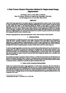
Figure 1. Overview of the proposed image segmentation algorithm. H Color Histogram (1470 Bins)
Histogram Generation (Quantization)
S
Gray Histogram (8 Bins)
(a)
(b)
(c)
Figure 2. Comparison between segmentation results in two color space: (a) Original image, (b) segmentation in RGB color space, (c) segmentation in HSV color space. The segmentation algorithm is based on K-Means clustering.
systems which have few computational resources.
2. Proposed Image Segmentation Method
V
Figure 3. Histogram generation process in HSV color space.
gray and color histogram bins for clustering in HSV color space is developed, and the transform from RGB to HSV in [3] is adopted. Since the ranges of three dimensions in HSV color space are not the same (Hue: [0, 360◦], saturation: [0, 1], and value: [0, 1]), a quantization process is performed to normalize the values in each dimension:
An overview of the proposed algorithm can be illustrated in Fig. 1, and the steps in which will be explained in the following subsections.
2.1. Color Space Transform and Histogram Generation Choices of color space may have signi�cant in�uences on the result of image segmentation. There are many kinds of color space, including RGB, YCbCr, YUV, HSV, CIE L*a*b*, and CIE L*u*v*. Although RGB, YCbCr, and YUV color spaces are commonly used in raw data and coding standards, they are not close to human perceptions. Besides, CIE color spaces are perceptually uniform but inconvenient since they require complicated computations. HSV (Hue, Saturation, Value) [16], which is shown to have better results for image segmentation than RGB color space [6, 19], is capable of emphasizing human visual perception in hues and has an easily invertible transform from RGB [3]. A comparison between segmentation results in RGB and HSV color space is shown in Fig. 2. Nevertheless, to our best knowledge, clustering in HSV color space is still an open question since there is no appropriate criteria for separation or distance measurement of gray and color pixels. Based on these observations, a new method that combines
h� = �Hue/hQ � ,
(1)
s = �Saturation/sQ � , v � = �Value/vQ � ,
(2) (3)
�
where (h� , s� , v � ) denotes the quantization index, and the quantization parameters hQ = 12◦ , sQ = 0.125, vQ = 0.125 are set empirically to accentuate the importance of hue and to save computational costs. Therefore, the HSV color space are divided into 30 × 8 × 8 = 1920 partitions. However, the hue of pixels with low saturation is often meaningless since their color is close to gray, and it is suggested that color histogram bins and gray histogram bins should be separated for better color representation [17, 19]. G(v) represents the number of pixel in the gray histogram bin with parameter v, whereas B(h, s, v) represents the number of pixel in the color histogram bin with parameters (h, s, v). The correspondence of these parameters and the quantization indices (h� , s� , v � ) are summarized in Table 1. Totally NG gray histogram bins and NB color histogram bins are generated, where NG = 8 and NB = 30 × 7 × 7 = 1470. The process of histogram generation and quantization is illustrated in Fig. 3. 855
2.2. Maximin Initialization and Parameter Estimation
Next, classify each color histogram bin to its nearest cluster centroid by the distance measurement. Thus the membership function of histogram bin Bi is de�ned by � (t) 1, if j = arg min D2 (Bi , Ck ) (t) k φ(j|Bi ) = . (6) 0, otherwise.
In traditional K-Means algorithm, cluster number K is often speci�ed by users, and the initial centroid positions are chosen randomly. In the proposed method, the parameters, including cluster number and the initial positions of cluster centroids, are all estimated through the Maximin algorithm [12] in a systematic approach. Three steps of the proposed Maximin algorithm, which are used in the preliminary stage for K-Means, are brie�y stated as follows: Step A: From the color histogram bins and gray histogram bins, �nd the bin which has the maximum number of pixels to be the �rst centroid. Step B: For each remaining histogram bin, calculate the min distance, which is the distance between it and its nearest centroid. Then the bin which has the maximum value of min distance is chosen as the next centroid. Step C: Repeat the process until the number of centroid equals to KMax or the maximum value of the distance in Step B is smaller than a pre-de�ned threshold, T hM . The threshold KMax = 10 is set based on the assumption that there should be no more than 10 dominant color in one image for high-level image segmentation, and T hM = 25 is set empirically according to the human perceptions of different color in HSV color space. The distance measurements of histogram bins and centroid vectors will be explained in Sec. 2.3.
On the other hand, for gray histogram bins, there is no hue information inside. Thus the distance measurement between a gray histogram bin Gi = (vi ) and a cluster centroid (t) (t) (t) (t) vector Cj = (hj , sj , vj ) is different from (4): (t)
The proposed K-Means clustering in HSV color space includes �ve steps, which are listed as follows: Step 1: Estimate the parameters of K-Means, including suitable value of K and the position of K initial cluster centroids from the Maximin algorithm in Sec. 2.2. Step 2: Two kinds of histogram bins will be clustered together in this step. For color histogram bins, since the hue dimension is circular (e.g. 0◦ = 360◦), the numerical boundary should be considered in the distance measurement and the process of centroid calculations. The distance measurement between a histogram bin vector Bi = (hi , si , vi ) (t) (t) (t) (t) and a cluster centroid vector Cj = (hj , sj , vj ) in the current iteration t is de�ned in the form of the Euclidean distance (2-Norm): D
(t) (Bi , Cj )
=
(t) Dh2 (hi , hj )
+ (si −
(t) sj )2
+ (vi −
N B � (t+1) hj
N B � (t+1)
sj
(t) vj )2 ,
=
N B � i=1 N B �
=
(t)
◦
(t)
2 ( 360 hQ − |hi − hj |) , if |hi − hj | > (t)
(hi − hj )2 ,
=
˜ (t) φ(t) B(Bi ) h i,j (j|Bi )
i=1 N B �
i=1
where �
(7)
and the values in each dimension of all centroid vectors for (t+1) the next iteration Cj are updated according to the following equations:
(4)
(t) Dh2 (hi , hj )
(t)
which means that the saturation values of gray histogram bins are all considered as zero, and the hue values can be arbitrary. Actually, gray level histogram bins can be regarded as “two-dimensional points” in a three-dimensional HSV space, and it is one of the main difference that the proposed K-Means algorithm, which operates across different dimensions, is different from others. Besides, the membership function of the gray histogram bin Gi is of the same form as (6), where Bi is replaced by Gi . Step 3: Recalculate and update K cluster centroids. Again, since the hue dimension is circular, the indices in the hue dimension should be considered not absolutely but relatively. An ef�cient method is introduced to calculate the relative hue index of the original hue index hi to the cen(t) (t) (t) (t) troid Cj = (hj , sj , vj ): ⎧ (t) (t) 360◦ 180◦ 180◦ ⎪ ⎨ hi − hQ , if |hi − hj | > hQ and hj < hQ ◦ (t) (t) ˜ (t) = 180◦ 180◦ , h hi + 360 i,j hQ , if |hi − hj | > hQ and hj > hQ ⎪ ⎩ hi , otherwise. (8)
2.3. K-Means Clustering in HSV Color Space
2
(t)
D2 (Gi , Cj ) = (sj )2 + (vi − vj )2 ,
180◦ hQ
otherwise.
(t+1)
vj ,
=
i=1
(t)
+
N �G i=1
(t)
vi φ(j|Bi ) B(Bi ) +
i=1
(9)
(t)
si φ(j|Bi ) B(Bi )
(t) φ(j|Bi ) B(Bi )
i=1 N B �
,
φ(j|Bi ) B(Bi )
(t) φ(j|Bi ) B(Bi )
+
,
(t)
(10)
φ(j|Gi ) G(Gi )
N �G i=1 N �G i=1
(t)
vi φ(j|Gi ) G(Gi ) (t) φ(j|Gi ) G(Gi )
,
(11)
(5) 856
where B(Bi ) denotes the number of pixels in the color histogram bin with histogram bin vector Bi , and G(Gi ) denotes the number of pixels in the color histogram bin with histogram bin vector Gi . Note that the range of hue value of the new centroid should be normalized in the range of [0, 360◦/hQ ). Step 4: Check if the clustering process is converged according to the total distortion measurement, which is the summation of distances between each histogram bin and its nearest cluster centroid: Δ(t) = +
N K B � � i=1 j=1 N K G � � i=1 j=1
(t)
Feature Extraction Query Image (RGB) Color Image Segmentation (Labeled Image) Texture Feature Database
Texture Feature Extraction
(Vector)
(Vector) Retrieval Similarity Measurement
(t)
φ(j|Bi ) D2 (Bi , Cj )B(Bi ) (t) (t) φ(j|Gi ) D2 (Gi , Cj )G(Gi )
.
Ranking
(12)
Results
When the difference of total distortion measurement |Δ(t+1) − Δ(t) | is smaller than a pre-de�ned threshold or when the maximum iteration number is reached, the iteration is terminated. Otherwise, return to Step 2 and t is incremented. Step 5: Image pixels are labeled with the index of the nearest centroid of their corresponding histogram bins. A labeled image l(x, y) is obtained in this step, and K-Means clustering is �nished.
2.4. Post-Processing of Spatial Regions For applications to extract spatial region information from image segmentation, elimination of noise and unnecessary details in labeled images is necessary. An ef�cient statistical �lter is introduced, and local histogram for a pixel on the position (x, y) in the labeled image is de�ned as � H(z|x, y) = 1, (13)
Figure 4. Overview of the CBIR system based on texture feature.
which is illustrated in Fig. 4. The post-processing step of image segmentation is ignored in this technique since the details of images should be preserved for texture feature. The proposed algorithm is based on the concept of Haar wavelet transform, and texture feature extraction using Discrete Wavelet Transform (DWT) [12] and the proposed algorithm, Label Wavelet Transform (LWT), will be introduced respectively in the following subsections.
3.1. Texture Feature based on Discrete Wavelet Transform The two-dimensional Discrete Wavelet Transform (DWT) is computed by applying a separable �lter bank to the gray level image [10, 22]:
l(x� ,y � )∈W(x,y) l(x� ,y � )=z
where W(x, y) is an N × N window centered in the spatial coordinate (x, y). Then the processed labeled image ˆl(x, y) is obtained by using the following equation: ˆ l(x, y) = arg max H(z|x, y). z
(14)
The purpose of this �lter is to replace the pixel in the labeled image with the label with maximum number in a window. Afterwards, the spatial regions (8-connected) whose area is smaller than a pre-de�ned threshold, T hA , are merged to the neighboring region with the maximum area to avoid over-segmentation.
3. Proposed Texture Feature Extraction Technique The proposed texture feature extraction method is constructed on a CBIR system based on image segmentation,
Dn,0 = [Hx ∗ [Hy ∗ Dn−1,0 ]↓2,1 ]↓1,2 ,
(15)
Dn,1 = [Hx ∗ [Gy ∗ Dn−1,0 ]↓2,1 ]↓1,2 ,
(16)
Dn,2 = [Gx ∗ [Hy ∗ Dn−1,0 ]↓2,1 ]↓1,2 ,
(17)
Dn,3 = [Gx ∗ [Gy ∗ Dn−1,0 ]↓2,1 ]↓1,2 ,
(18)
where H and G are the low-pass and high-pass �lter respectively, and the symbol ∗ denotes the convolution operator, ↓2 ,1(↓1,2) denotes sub-sampling along the rows (columns) by a factor of two. Dn,0 is obtained by low-pass �ltering the original image n times, and it is also referred to as the low resolution image at scale n. The detail images Dn,1 , Dn,2 , and Dn,3 are obtained by band-pass �ltering in a speci�c direction, and they can be categorized into three frequency bands: HL, LH, HH band, respectively. Each band contains different directional information at scale n. For example, 857
(a)
−1 [ √12 , √ ] are applied to each 2 × 2 pixel block partitioned 2 from the gray level image. Floating point multiplications or integer multiplications with divisions are needed in DWT, and these operations are inef�cient for the real-time processing demand. Therefore, the proposed algorithm, Label Wavelet Transform (LWT), concentrates on providing a fast texture feature extraction method on the labeled image from image segmentation. An illustration of a three-level LWT is shown in Fig. 5. For a labeled image from segmentation, it is meaningless to directly apply DWT since these labels represent the cluster label of the pixels, which only reveals whether neighboring pixels belong to the same cluster or not. In order to extract texture feature in the horizontal, vertical and diagonal directions of the labeled image, low-pass and high-pass �lters used in the Haar wavelet transform are implemented by down-sampling and calculating the number of neighboring label changes in the three directions (horizontal, vertical and diagonal) in the labeled image. The measurement of the texture feature is de�ned as follows:
(b)
LL3 HL3 HL2 LH3 HH3
LH2
HL1 HH2
LH1
HH1
(c)
(d)
W
Figure 5. Illustration of the proposed texture extraction method, Label Wavelet Transform (LWT): (a) the original image, (b) the labeled image after segmentation, and (c)(d) three level decomposition of LWT. Each pixel in the segmentation image is represented by the color of its cluster centroid, and down-sampled binary images of four frequency bands (LL, LH, HL, HH) can be obtained in each layer.
the HL band shows variations in the horizontal direction. Thus an image with vertical lines results in high energy in the HL band and low energy in the LH band. The �lter bank employed is based on the Haar wavelet for its ef�ciency and localization [21]. The texture feature is extracted from the 2 variance σn,i of the coef�cients cn,i of the detail images Dn,1 , Dn,2 , and Dn,3 at different scale n: � 1 2 = c2n,i (k, l) − μ2n,i . (19) σn,i #Dn,i (k,l)∈Dn,i
where μn,i denotes the mean value of cn,i . To represent the texture feature of an image q, the texture feature vector of DWT is de�ned as [12]: 2 2 2 2 TDW T (q) = [σ1,1 , σ1,2 , σ1,3 , ..., σN ], max ,3
(20)
where Nmax denotes the largest scale. In this work, Nmax = 3 [18] is chosen according to the size of testing images, and a 9-component texture feature vector is used to represent each image.
3.2. Proposed Technique based on Label Wavelet Transform In the Haar transform, which is the fastest Discrete Wavelet Transform (DWT) [21], the low-pass �lter with coef�cients [ √12 , √12 ] and the high-pass �lter with coef�cients
Hn,1
H
1 � 2 −1 � 2 −1 � = (Ln−1 (2k, 2l + j)⊕ j=0 k=0
l=0
Ln−1 (2k + 1, 2l + j)), W
Hn,2
H
1 � 2 −1 � 2 −1 � = (Ln−1 (2k + j, 2l)⊕ j=0 k=0
l=0
Ln−1 (2k + j, 2l + 1)), W
Hn,3
(21)
(22)
H
−1 2 −1 1 � 2 � � = (Ln−1 (2k + j, 2l)⊕ j=0 k=0
l=0
Ln−1 (2k − j + 1, 2l + 1)),
(23)
where Ln−1 is the (n − 1)-th level labeled image obtained by down-sampling the original labeled image L0 n − 1 times, W and H represent the width and height of Ln−1 respectively, the symbol ⊕ represents the exclusive-or operation, and Hn,1/2/3 is the n-th level measure of the horizontal/vertical/diagonal label dissimilarity in the labeled image. It is observed that only the logic operations (exclusive-or) and additions are needed for the computation in LWT, and neither multiplications nor divisions are required. The histograms of the label changes in three different directions (horizontal, vertical, and diagonal) are calculated and are then treated as the texture feature since texture is a property of the homogeneity and variations in a region. For the purpose of comparing the retrieval results with that of DWT feature, the representation form of LWT feature vector of an image q is similar to (20): TLW T (q) = [H1,1 , H1,2 , H1,3 , ..., HNmax ,3 ], 858
(24)
10000 Number of Region
200 4
Distortion (x10 )
Random Autonomous
100
0
kodim01 kodim03 kodim07 kodim22
1000
100
10 1
6
11
16 Iteration
21
26
0
2
4 6 Filter Window Size
(a)
8
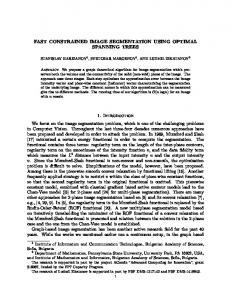
10
Figure 6. (a) Total distortion v.s. iteration of K-Means with image kodim03. (b) Region number v.s. �lter window size with four images.
where Nmax denotes the largest scale. In this work, Nmax = 3 is chosen according to the size of testing images, and a 9-component texture feature vector is used to represent each image.
3.3. Retrieving Process To focus on the comparison between the performance and processing speed of the Haar wavelet-based method and the proposed approach, only texture feature is used for image retrieval. In the retrieving process, the dissimilarity between the query image q and each image in database Ij is measured by the Euclidean distance (2-Norm): 2
D (q, Ij ) =
(a)
(b)
(c)
(b)
N� 3 max �
(T (q)n,i − T (Ij )n,i )2 ,
(25)
n=1 i=1
where T (.)n,i denotes the element with subscript (n, i) in the texture feature vector TDW T (.) or TLW T (.): namely, 2 σn,i in the Haar wavelet-based method (DWT) and Hn,i in the the proposed approach (LWT). The CBIR system obtains the retrieval results by using the nearest neighbor algorithm based on the distance measurement in (25), and the database images are then retrieved according to their rankings of distance, with the one having the highest ranking being retrieved �rst.
4. Experimental Results The experiments are performed in Pentium-D 2.66GHz computer with 2GB memory, and they are conducted based on two contributions of this work: the fast image segmentation and the ef�cient texture extraction method.
4.1. Fast Color Image Segmentation The experiments of image segmentation contain three parts. The �rst part is algorithm comparison. Totally 525 images are tested, and for 25 images of size 768 × 512, the average execution time of the proposed method is 0.29 second, whereas the method in [19] requires 1.20 second. Also, the clustering result of these two methods are shown in Fig. 7, where the method in [19] separates color and gray
Figure 7. Image kodim06: (a) the original image, (b) the clustering result of the proposed method , and (c) the clustering result in [19], where color and gray pixels are separated deterministically and marked. Table 2. Mean Average Precision (MAP) and Feature Extraction Time (FET) Comparison between DWT and LWT
Category
Beach Building
Bus
Flower Food Average
MAP (DWT/LWT)
1.15
1.02
1.10
0.98
1.16
1.075
FET (DWT/LWT)
15.37
14.27
11.58
14.55
21.78
15.51
Total FET (DWT/LWT)
3.17
3.19
2.75
2.93
4.02
3.21
pixels in HSV color space deterministically, and the proposed method clusters color and gray pixels together. It can be seen that the proposed method obtains better results than the method in [19] in terms of speed and robustness. The second part is the functionality testing of the proposed K-Means clustering. To ensure K-Means operates properly in HSV color space with gray histogram bins and color histogram bins, the total distortion measurement in (12) is plotted with respect to iteration times. It is found that for all testing images, the distortion declines as the iteration time increases. Also, the Maximin initialization can obtain distortions similar to the random initialization: A plot of image kodim03 is shown in Fig. 6(a), where the distortions of random initialization are average values in ten times. The third part is the performance analysis for postprocessing. To test if the proposed �lter can effectively reduce the region number of the labeled image, the relation of region (8-connected) number and �lter window size with four testing images are plotted in Fig. 6(b). It can be seen that the region number declines dramatically as the window size N increases.
4.2. Ef�cient Texture Feature Extraction In the experiment of texture feature extraction, the COREL database [20] is used instead of the Brodatz texture gallery [1] for the reason that this work focuses on color images which are more likely to appear in the real-world applications. The COREL database includes ten categories with each category having 100 images, and �ve categories among them are selected. The other �ve categories are not selected since it is observed that the common texture feature in these categories are not obvious. Example images 859
of the selected categories and their segmentation results are shown in Fig. 8, where the category “Beach” has smooth textures in the sky and the sea region, the category “Building” has lots of vertical and horizontal edges, the category “Bus” has diagonal edges at the boundaries of vehicles, the category “Flower” has large scale textures in petal regions, and the category “Food” consists of irregular texture patterns. To evaluate the performance of the retrieval system, two measurements: recall and precision [15] are used for the construction of precision-recall curve (PR curve). The experiment contains two parts, one is the analysis of PR curve for each category, and the other is the comparison of the average performance and processing speed between DWT [12, 18] and the proposed LWT. Every image in the selected �ve categories is treated as an individual query, and images in the same category of the query are its relevant database. precision and recall are calculated for every query, and they are averaged to obtain the PR curve for each category. The results are shown in Fig. 9, and it is observed that the distortion between DWT and LWT in these �ve categories is small. Besides, the comparison of the precision and the processing speed between the Haar wavelet-based feature (DWT) and the labeled imagebased feature (LWT) is listed Table 2, where three measurements: “MAP,” “FET,” and “Total FET” are used. “MAP” is the abbreviation of “Mean Average Precision,” which is the average precision of �ve categories, and “FET” stands for “Feature Extraction Time” to extract the texture feature. Moreover, “Total FET” considers total feature extraction time for both algorithms: for DWT, the time of gray level transform is included; for LWT, the time of color image segmentation is included. From Table 2, it is observed that the average texture feature extraction speed (FET) of LWT is 15.51 times faster than that of DWT. Moreover, by comparing “Total FET,” the speed of LWT is still 3.31 times faster than DWT. For the quality of the retrieval results using LWT, there is only 6.9% loss of average precision over the �ve categories compared with DWT. Since labeled images of segmentation contain less information than gray scale images, it is reasonable that the performance of LWT is lower than DWT. In summary, the experiments demonstrate that the proposed method, LWT, can greatly increase the texture feature extraction speed while keeping the distortion within a reasonable range, and it effectively provides the trade-off between the performance and the texture feature extraction time.
5. Conclusion There are mainly two contributions in this paper: one is the fast image segmentation method, and the other is the ef�cient texture extraction method. The characteristics of the proposed image segmentation method include a new quan-
(a)
(b)
(c)
(d)
(e)
(f)
(g)
(h)
(i)
(j)
Figure 8. Example images from �ve selected categories in the COREL gallery: (a) Beach, (c) Building, (e) Bus, (g) Flower, and (i) Food. The corresponding labeled image obtained from segmentation (without post-processing): (b) Beach, (d) Building, (f) Bus, (h) Flower, and (j) Food.
tization method to generate gray and color histograms in HSV color space for K-Means clustering, where the cluster number is automatically estimated based on Maximin initialization. The segmentation method is both fast and ef�cient to extract regions with different colors in images, and the results are close to human perceptions. In addition, the proposed texture extraction method, Label Wavelet Transform (LWT), can be regarded as an application of image segmentation. Different from existing methods, it utilizes the information from segmentation and applies only exclusive-or and addition operations to extract texture feature from the labeled image. This algorithm provides a fast and ef�cient way towards texture feature extraction. It is especially useful in the on-line retrieval system with real-time demands in embedded systems. 860
1
1 Haar Proposed
0.8
0.7
0.7
0.6
0.6
0.5 0.4 0.3
0.1 0.02
0.03
0.04
0.05
0.06
0.07
0.08
0.09
0 0.01
0.1
0.02
0.03
0.04
(a)
(b)
1
0.07
0.08
0.09
0.1
[9]
1 Haar Proposed
0.9
0.7
0.7
0.6
0.6
Precision
0.8
0.5 0.4 0.3
[10]
Haar Proposed
0.5 0.4 0.3
0.2
0.2
0.1
[11]
0.1 0.02
0.03
0.04
0.05
0.06
0.07
0.08
0.09
0 0.01
0.1
0.02
0.03
0.04
Recall
0.05
0.06
0.07
0.08
0.09
0.1
Recall
(c)
(d)
1
1 Haar Proposed
0.9
Haar Proposed
0.9
0.8
0.8
0.7
0.7
0.6
0.6
Precision
Precision
0.06
Recall
0.8
0.5 0.4 0.3
[12]
0.5 0.4 0.3
0.2
[13]
0.2
0.1 0 0.01
0.05
Recall
0.9
Precision
0.4
0.2
0.1
0 0.01
[8]
0.5
0.3
0.2
0 0.01
Haar Proposed
0.9
0.8
Precision
Precision
0.9
0.1 0.02
0.03
0.04
0.05
0.06
Recall
(e)
0.07
0.08
0.09
0.1
0 0.01
0.02
0.03
0.04
0.05
0.06
0.07
0.08
0.09
0.1
Recall
(f)
Figure 9. PR curve of �ve categories: (a) Beach, (b) Building, (c) Bus, (d) Flower, and (e) Food. (f) Average PR curve of these �ve categories.
[14]
[15]
References [1] P. Brodatz. Textures: A Photographic Album for Artists and Designers. Dover Publications, Inc., New York, 1966. 6 [2] C. Carson, M. Thomas, S. Belongie, J. M. Hellerstein, and J. Malik. Blobworld: A system for region-based image indexing and retrieval. In Proceedings of Third International Conference on Visual Information Systems, pages 509–516, 1999. 1
[16]
[17]
[18]
[3] W. Chen, Y. Q. Shi, and G. Xuan. Identifying computer grahics using HSV color model and statistical moments of characteristic functions. In Proceedings of IEEE International Conference on Multimedia and Expo, pages 1123– 1126, July 2007. 2
[19]
[4] A. Dong and B. Bhanu. Active concept learning in image databases. IEEE Transactions on Systems, Man, and Cybernetics, Part B, 35(3):450–466, June 2005. 1
[20]
[5] R. M. Haralick. Statistical and structural approaches to texture. Proceedings of the IEEE, 67(5):786–804, May 1979. 1 [6] Z.-K. Huang and D.-H. Liu. Segmentation of color image using EM algorithm in HSV color space. In Proceedings of IEEE International Conference on Information Acquisition, pages 316–319, July 2007. 2
[21]
[22]
[7] M. Kokare, P. K. Biswas, and B. N. Chatterji. Texture image retrieval using new rotated complex wavelet �lters. IEEE
861
Transactions on Systems, Man, and Cybernetics, Part B, 35(6):1168–1178, Dec. 2005. 1 S. Livens, P. Scheunders, G. V. D. Wouwer, and D. V. Dyck. Wavelets for texture analysis, an overview. Proceedings of Sixth International Conference on Image Processing and Its Applications, 2:581–585, July 1997. 1 W.-Y. Ma and B. S. Manjunath. NeTra: A toolbox for navigating large image databases. Multimedia Systems, 7(3):184–198, 1999. 1 S. G. Mallat. A theory for multiresolution signal decomposition: The wavelet representation. IEEE Transactions on Pattern Analysis and Machine Intelligence, 11(7):674–693, 1989. 4 B. S. Manjunath and W. Y. Ma. Texture features for browsing and retrieval of image data. IEEE Transactions on Pattern Analysis and Machine Intelligence, 18(8):837–842, Aug. 1996. 1 V. Mezaris, I. Kompatsiaris, and M. G. Strintzis. Still image segmentation tools for content-based multimedia applications. International Journal of pattern recognition and arti�cial intelligence, 18(4):701–725, June 2004. 3, 4, 5, 7 M. Ozden and E. Polat. A color image segmentation approach for content-based image retrieval. Pattern Recognition, 40(4):1318–1325, 2007. 1 Y. Rui, T. S. Huang, and S.-F. Chang. Image retrieval: Current techniques, promising directions, and open issues. Journal of Visual Communication and Image Representation, 10(1):39–62, Mar. 1999. 1 A. W. M. Smeulders, M. Worring, S. Santini, A. Gupta, and R. Jain. Content-based image retrieval at the end of the early years. IEEE Transactions on Pattern Analysis and Machine Intelligence, 22(12):1349–1380, Dec. 2000. 7 J. R. Smith. Color for image retrieval. In Image Databases, chapter 11, pages 285–311. John Wiley & Sons, Inc., 2002. 2 J. R. Smith and S.-F. Chang. Single color extraction and image query. In Proceedings of IEEE International Conference on Image Processing, pages 528–531, Oct. 1995. 2 N. Suematsu, Y. Ishida, A. Hayashi, and T. Kanbara. Regionbased image retrieval using wavelet transform. In Proceedings of 10th International Workshop on Database and Expert Systems Applications, pages 167–173, 1999. 5, 7 S. Sural, G. Qian, and S. Pramanik. Segmentation and histogram generation using the HSV color space for image retrieval. In Proceedings of IEEE International Conference on Image Processing, pages 589–592, Sept. 2002. 2, 6 J. Z. Wang, J. Li, and G. Wiederhold. SIMPLIcity: Semantics-sensitive integrated matching for picture libraries. IEEE Transactions on Pattern Analysis and Machine Intelligence, 23(9):947–963, 2001. 1, 6 X. Wen, T. D. Huffmire, H. H. Hu, and A. Finkelstein. Wavelet-based video indexing and querying. Multimedia System, 7(5):350–358, 1999. 5 G. V. D. Wouwer, P. Scheunders, and D. V. Dyck. Statistical texture characterization from discrete wavelet representations. IEEE Transactions on Image Processing, 8:592–598, 1999. 1, 4