IEEE Transactions on Automation Science and Engineering
1
Fast Intersection-free Offset Surface Generation from Freeform Models with Triangular Meshes Shengjun Liu and Charlie C.L. Wang, Member, IEEE Abstract—A fast offset surface generation approach is presented in this paper to construct intersection-free offset surfaces, which preserve sharp features, from freeform triangular mesh surfaces. The basic spirit of our algorithm is to sample a narrowband signed distance-field from the input model on a uniform grid and then employ a contouring algorithm to build the resultant offset mesh surface from the signed distance-field. Four filters are conducted to generate the narrow-band signed distance-field around the offset surface in a very efficient way by alleviating computation redundancies in the regions far from the offset surfaces. The resultant mesh surfaces are generated by a modified dual contouring algorithm which relies on accurate intersections between the grid edges and the isosurfaces. A hybrid method is developed to prevent the expensive bisection search in the configurations that the analytical solutions exist. Our modified intersection-free dual contouring algorithm is based on convexconcave analysis, which is more robust and efficient. The quality and performance of our approach are demonstrated with a number of experimental tests on various examples. Note to Practitioners—This research is motivated by the problem about how to generate intersection-free offset surfaces from a general freeform model bounded by triangular mesh surfaces. Current commercial 3D/2D Computer-Aided Design and Manufacturing (CAD/CAM) systems cannot support the offsetting operation on a general freeform 3D model. This paper presents a new approach which considers the problem in a different manner. Firstly, the offset surfaces are sampled into an implicit representation – a narrow-band signed distance-field. Secondly, the distance-field is contoured into an intersection-free mesh surface that gives the approximated offset surface. The approach can be integrated into commercial CAD/CAM systems to enrich their offsetting functions which are widely used in various CAD/CAM applications, such as filleting, rounding and hollowing of 3D models, tolerance and clearance analysis for assembly, coordinate measuring machines (CMM), tool path generation for 3D numerically controlled (NC) machining, and robot path planning. Index Terms—Offset surface generation; freeform surface; signed distance field; filtering; intersection-free
Shengjun Liu is now with School of Mathematical Science and Computing Technology, Central South University, China. This work was completed when he was with the Department of Mechanical and Automation Engineering, The Chinese University of Hong Kong, Shatin, NT, Hong Kong. Charlie C.L. Wang (Corresponding Author) is with the Department of Mechanical and Automation Engineering, The Chinese University of Hong Kong, Shatin, NT, Hong Kong (Tel: (852) 2609 8052; Fax: (852) 2603 6002; E-mail:
[email protected])
I. INTRODUCTION
O
FFSET surface generation is an important operation in many CAD/CAM applications. An offset surface of a solid H is the set of points having the same offset distance r from the boundary ∂H of H. When considering the sign of distances, we can have a grown offset H r with the points on
H r being outside of H and a shrunk offset surface H r that has all its points inside the solid H. Problem Definition: Given a solid model H with its boundary surface ∂H represented by a triangular mesh, the boundary mesh surface of H r (or H r ) is to be computed. Although the offsetting operation is mathematically well defined [1], offsetting a solid model exactly has proven to be difficult. In general, for a polygonal mesh, the Minkowski sum of it with a sphere is decomposed into a set of spheres, cylinders, and prisms corresponding to vertices, edges, and faces of the mesh. A constructive solid geometry approach to offset surface computation is based on computing the union of all these elements. However, the computation for the union operations of these solids has been proven difficult because of its computational complexity and numerical instability [1-3]. In recent years, volumetric approaches (e.g., [4, 5]) and pointbased algorithm [6] have been proposed to overcome these difficulties. These algorithms first generate volumetric grids and sampling points to approximate the offset model and then employ a distance-field or collision detection technique to calculate the resultant implicit surface or sample points. However, they usually suffer the problems of missing sharp features (e.g., [4, 6]) or long computing time (e.g., [4], [5]). Our method for offset surface generation can also be classified as a volumetric approach. According to the offset surface‟s intrinsic property that every point on the offset surface with an offset value r has a minimal distance | r | to the original mesh, we use a distance function to define the offset surface directly on triangles. Specifically, an offset surface of H with distance r can be implicitly defined by the following equation f ( p) dis( p, H ) r 0 , (1) where p is a point on the offset surface of the given model H in R3, and dis(…) is a function returning the signed distance with „+‟ representing a point outside H and „–‟ for a point inside.
IEEE Transactions on Automation Science and Engineering The offset value r can be either positive or negative. The signed distance-field is sampled on uniform grids in a narrowband manner – i.e., accurate distances are only computed on the grid nodes near the offset surface. Efficient algorithm for constructing such a signed distance-field is developed by introducing four filters that can greatly alleviate the computational redundancy. As the mesh surface generated by the dual contouring (DC) algorithm [7] can automatically preserve sharp features, our distance-field is also converted into the final offset surface through a dual contouring step that needs to compute accurate intersections between the grid edges and the offset surface. A hybrid method is developed to prevent the expensive bisection search in the configurations that analytical solutions exist. To get a resultant mesh surface that has no self-intersection, we modify the intersection-free DC algorithm [8] by a convex/concave analysis, which is more robust and efficient. In short, the major contributions of our approach include: To identify the grid cells which are intersected by the offset surface and create a narrow-band signed distancefield quickly, four filters are introduced in section IV. The swept sphere volume hierarchy (SSVH) filter is adopted to filter out most of the triangles on the input model from the distance computation. A bounding box filter, a signed distance filter, and an octree filter are employed to filter out most of the grid nodes which are far from the offset surface. These filters can remove around 97% – 99.9% of the unnecessary distance computation on grid nodes. To employ the strategy of DC to generate the resultant meshes for offset surfaces, the intersections between the grid edges and the implicit offset surface must be computed. A straightforward way to compute them is by the bisection search, which however is very slow. We introduce a hybrid method in section V that combines the analytical solution (whenever is applicable) and the bisection search to compute the intersections. To reconstruct sharp features on the resultant offset mesh surfaces, every intersection point must be equipped with a normal vector, which can be determined by the closest point search. Although self-intersections of the offset solid have been automatically eliminated due to the distance-field based representation, they may be re-generated on the resultant mesh surfaces during the contouring procedure – see the discussion and the first approach to address this problem in [8]. We present a modified DC method based on convex/concave analysis (in section VI), which is more robust and efficient. II. RELATED WORK Offset operations can be considered as a special case of the Minkowski sum [1]. There are several approaches in literature for the evaluation of Minkowski sum on solid models. Varadhan et al. proposed a method in [4] to approximate the Minkowski sum of polyhedral models. This method avoids the
2 union step and its computation is simple and effective for convex objects. For general 3D polyhedrons, a divided-andconquer approach is employed where it first applies convex decompositions, then computes the pair-wise Minkowski sums between those convex pieces, and finally extracts the boundary from the union of all the pairwise Minkowski sums [9]. However, such decomposition is not easy for complex objects [10] and makes too many components. In order to avoid the last union step among a number of components, a distancefield based method is employed in [4], which however has difficulty to reconstruct sharp features. Recently, Zhang et al. [11] generate the resultant boundary surface from sweeping volume with a dual-contouring like approach to retain shape features. However, self-intersections may happen (as discussed in [8]). Moreover, the volumetric region of resultant solid is computed by a flooding algorithm in [11]. This will miss the inner voids that are very important for the shrunk offsetting operation. Pavic and Kobbelt [5] extract the boundary surfaces by a Marching Cubes (MC) like algorithm that does not generate self-intersection. However, sharp features cannot be automatically reconstructed and MC algorithm usually generates much more triangles than DC. A post-processing step is used to recover sharp features. This step however can lead to self-intersection on the resultant mesh surfaces. A point-based method is presented to robustly compute an approximate and accurate representation of the Minkowski sums boundary in [6]. Its resultant boundary is a point-based representation and will lose those small but important sharp features. These methods run much more slowly as they are not specially designed for offset surface generation. Offset operations can be applied to curves, surfaces, or entire 3D models. In earlier work [1], the mathematical basis for offsetting of solids was described. The offset techniques for curves and surfaces have been extensively studied by Pham [2] and Maekawa [3]. For 3D solid models, it will be more complicated to generate offsets, which involve not only the geometrical issue of offsetting each individual surface in the model but also the topological issue of reconnecting these offset surfaces into a closed 3D model. Generally, offsets of 3D models are achieved by first offsetting all surfaces of the model and then trimming or extending these offset surfaces to reconstruct a closed 3D model [1, 12, 13, 14]. These earlier approaches first compute a superset of the offset surface by offsetting 1) vertices into spheres, 2) edges into cylinders, and 3) faces into parallel faces. Then, they trim that superset by subdividing its elements at their common intersections and deleting the pieces that are too close to the original solid. This is a very expensive computing process and the trimming at tangential contacted regions is numerically unstable. The computation in our approach is much more stable since we work on a volumetric representation that can handle the tangential contact robustly. Some surface-based approaches for generating offset surfaces simply shift the original vertices in the offsetting direction [15]. This is problematic as selfintersections may occur either locally in areas of high
IEEE Transactions on Automation Science and Engineering
3
Fig. 1. The overview of our algorithm illustrated in 2D: (leftmost) the given model bounded by oriented two-manifold mesh surfaces, (left) the input model is embedded in a space that is sampled into uniform grids, (middle) classifying the grid nodes inside/outside the offset surface in a narrow-band manner – nodes that are not in the narrow-band region of the offset surface do not need to be considered, (right) intersections between the offset surface and the grid edges are computed, and (rightmost) the resultant offset mesh surface is extracted by an intersection-free dual contouring algorithm.
curvature or globally when different parts of the input surface meet during the vertex shifting. On the contrary, selfintersections are eliminated by our method since the volumetric representation and an intersection-free contouring method used in the surface extraction. There are many other methods for offset surface generation with the help of different representations. Volumetric methods were presented based on distance-fields and the fast marching method in [16, 17]. The approximation properties of the fast marching [18] do not allow for high accuracy. Recently, a point-based offsetting approach was introduced in [19], where point samples are first generated on the input surface and are then moved in normal direction. After that, the Minkowski sum volume is rasterized on voxel grids in order to remove self-intersections. In [20], another offsetting approach was presented which aims mainly at visualizing the offset via surface splats. In their cases, the classification on whether a cell intersects the offset surface is based on conservative estimates for both the minimum and maximum distance. While this is sufficient for visualization purposes, it would be nontrivial to extract a proper manifold offset surface from it. On the contrary, our method gives intersection-free mesh surfaces as the results. A hybrid method combining surface and volume was proposed in [5]. The algorithm is also based on computing the union of a set of primitives (spheres, cylinders and planes). Its computations are stable since the method works on a volumetric representation and the self-intersections can be easily removed by computing the min/max operations applied to distance functions. However, there are still some limitations of this method. The first one is that it generates two offset surfaces simultaneously without identifying the outer or inner ones. The second is the sharp feature extraction problem as aforementioned. Nevertheless, our method defines the offset surface in a narrow-band signed distance-field which results in an identical surface, and the sharp features are intrinsically preserved during the surface extraction. Another hybrid method which combines point and implicit surface was presented in [21]. This method reconstructs the zero-level surface and an offset surface simultaneously from an oriented point set. It first generates the offset point set, and then fits the
surfaces with an implicit function combining two point sets. It is stable and robust for different point data, such as noisy points and irregular points. However, using this method, the sharp features cannot be reconstructed, and there are large artifacts on the offset surface where there are no offset points from the sharp features on the original model when the offset distance is large. On the contrary, our method preserves the sharp features and provides highly accurate results even if the offset distance is very large. III. OVERVIEW Given a solid model bounded by oriented two-manifold meshes, our goal is to obtain its intersection-free offset surface with sharp features preserved. The whole algorithm consists of three steps. Firstly, the given model H is embedded into a space Ф bounding the model and its offset surfaces. The space Ф is sampled into a narrow-band signed distance-field on uniform grids, where the narrow-band region is around the offset surface but not the surface of H. Four filters are developed to efficiently evaluate the distance-field (see section IV). Secondly, the intersections between the grid edges and the offset surface are computed. We analyze the possible configurations of the intersections, and derive a more efficient method to compute the intersections analytically whenever possible (see section V). Lastly, a modified intersection-free dual contouring algorithm is introduced to extract the mesh of offset surfaces (see section VI). Our method is based on convex/ concave analysis, which is more robust and efficient. Figure 1 gives a 2D illustration of the overall algorithm. Our approach is simple and easy to implement. Moreover, as the narrow-band distance-field is sampled on uniform grids, the minimal distance evaluation and the intersection computation can be easily parallelized on PC with multi-core CPUs. IV. FILTERS FOR DISTANCE-FIELD CONSTRUCTION To construct a signed distance-field of a given model H sampled on a uniform grid with n × n × n grid nodes, the most
IEEE Transactions on Automation Science and Engineering straightforward method is to compute the minimal distance from these n3 nodes to the surface, ∂H, of H represented by triangular meshes. The minimal distance from a query point q to ∂H can be evaluated by an exhaustive search of all triangles on ∂H. After finding the closest point cq of q on ∂H, the sign of distance between cq and q is decided by the angle weighted pseudonormal on cq [22]. Although the sign of distance can be determined very efficiently, the computation of closest point is time-consuming – especially when such a distance computation is conducted on all n3 nodes with a large value of n (e.g., n = 513 as shown in our examples in this paper). Four filters are introduced in this section to speed up the evaluation. A. Swept Sphere Volume Hierarchy (SSVH) Filter The SSVH filter is applied to the triangles of ∂H to speed up the distance computation between a query point q and the triangles on ∂H. The basic idea is to establish a volume bounding hierarchy (BVH) of the triangles so that the computation on triangles that are far from the query point q can be discarded. The Swept Sphere Volume Hierarchy (SSVH) presented in [23] is adopted here as it can be easily modified to compute the minimal distance between a point and a set of polygons. Instead of computing the minimal distance between polygons, we employ a fast algorithm in [24] to compute the distance between the query point and a triangle, where the triangle is defined as t (u, v) b ue0 ve1 with the parametric domain D {(u, v) : u, v [0,1], u v 1} . The minimal distance is computed by finding the optimal parameters (u , v ) D that lead to the closest point to the query point q. Besides the minimal distance from q to ∂H, we also record the closest point cq, the triangle holding cq, the parameters (u , v ) for cq, and the sign of distance, which will be used in the following computations. B. Bounding Box Filter Although the evaluation of function f(p) using the SSVH filter is fast, the construction of a signed distance field is still time consuming since there are n3 nodes. Running on a PC equipped with Intel Core 2 CPU 6600 2.4GHz with 2GB RAM, the closest point computation using SSVH for a model with 400K triangles (i.e., the vase-lion model shown later in Fig.16) can be completed in 1.047ms on average. When computing the signed distances on 513 × 513 × 513 grid nodes, it takes 513 × 513 × 513 × 1.047ms ≈ 39.26 hr, which is impractical. A wiser solution is to construct a narrow-band distance field around the offset surface of H. Without loss of generality, the offset surface is located in a narrow-band region of the grid cells. Definition 1 For any grid node, if its position p satisfies dis( p, H ) r l
(2)
with l being the width of grid boxes, this grid node is adjacent to the r-offset surface and defined as valid grid nodes. For a grid node not agreeing with Eq.(2), it is called an invalid
4
Fig. 2. Illustration of the bounding box filter in 2D with d = | r |. The bold black line represents the surface of the given mode, and the two bold red lines refer to the grown and the shrunk offset surfaces. The grid nodes in a bounding box, the center of circumsphere that does not fall in the purple regions, are invalid grid nodes – illustrated by empty circular dots. The black circular dots are candidates of valid grid nodes.
grid node. In the middle figure of Fig.1, only the valid nodes are displayed with small cubes. However, directly checking whether a grid node is valid also involves the distance computation between a point and the given triangular meshes. To avoid redundant evaluation, we introduce the bounding box filter below. The grid cells are grouped into cubic bounding boxes with a larger size, where each bounding box consists of m × m × m grid boxes (i.e., including (m+1)3 grid nodes). The uniform grids become (n 1) m (n 1) m (n 1) m bins. Remark 1 For a sphere with radius δ, if the minimal distance from its center sc to the boundary surface of H satisfies dis(sc , H ) r l , (3) all grid nodes in this sphere must be invalid. The radius of the circumsphere for a bounding box is
3ml 2 , therefore we can use the above remark to detect whether the grid nodes in a bounding box are invalid with 3ml 2 . Checking remark 1 directly needs to compute the signed distances on all bounding boxes. To speed up the computation, in the bounding box filter, we compute the unsigned distance, undis(sc, ∂H), between the center of the circumsphere of a bounding box and the surface ∂H. If the circumsphere of a bounding box agrees with undis(sc , H ) d l where d = | r |, its corresponding signed distance must satisfy Eq.(3) – such a bounding box is named as invalid bounding box; otherwise, it is called valid bounding box. Remark 2 All grid nodes in an invalid bounding box must be invalid, but the grid nodes in the valid bounding box could be either valid or invalid. Figure 2 gives an illustration of the bounding box filter. Note that, the grid nodes around both the grown and the shrunk offset surfaces remain after applying this filter. C. Signed Distance Filter To retain only the bounding boxes around the grown offset
IEEE Transactions on Automation Science and Engineering
5
Fig. 3. Two configurations when applying the signed distance filter to grown offsetting – two band regions are (a) separated and (b) overlapped.
surface (or the shrunk surface), we check the signed distance dis(sc, ∂H) of the valid bounding boxes by a signed distance filter using the remarks below. Remark 3a For the distance-field for a grown offset surface (r > 0), the grid nodes in a bounding box satisfying dis(sc , H ) d l , min(d l , d l ) (4) are invalid, where d = | r | and sc is the center of the bounding box‟s circumsphere. Remark 3b For the distance-field for a shrunk offset surface (r < 0), if a bounding box satisfies dis(sc , H ) max(d l ,d l ), d l , (5) all grid nodes in it are invalid. Here, the invalidity of a grid node refers to the inability to satisfy Eq.(2) in Definition 2. The min(…) and max(…) functions in remark 3 are caused by the configuration that the two band regions overlap when the offset distance d is very small. Figure 3 shows two configurations when applying the signed distance filter for the grown offsetting. D. Octree Filter The bounding box filter and the signed distance filter introduced above can fast recognize many invalid grid nodes. However, when choosing a large bounding box size, many invalid grid nodes survive since they are enclosed by a valid bounding box (see Fig.4(a) for an example). To further exclude the invalid grid nodes from the narrow-band signed distance-field, an octree filter is introduced. Starting from a retained bounding box, we recursively subdivide the bounding box into eight sub-boxes. For each sub-box B, the signed distance disB from the center of its circumsphere to ∂H is computed. If the signed distance disB agrees with Eq.(3), the recursive subdivision on this sub-box is stopped, and all grid nodes in this sub-box are classified as invalid. Those grid nodes located on the interface of several sub-boxes are marked as invalid if the signed distance from any center of these subboxes‟ circumspheres agrees with remark 3. Figure 4(b) gives the illustration of octree filtering on a retained bounding box. V. SURFACE INTERSECTIONS ON GRID EDGES After applying the above four filters, we can efficiently construct a narrow-band signed distance-field around the offset
Fig. 4. Using an octree filter to further detect the validity of grid nodes in the retained bounding boxes: (a) the bounding box is valid but the enclosed grid nodes are invalid, and (b) invalid grid nodes are excluded recursively in the octree filter.
surface f(p) = r. The signed distances are only evaluated on the valid grid nodes. By the local signed distances, we can detect the grid cells intersecting with the offset surface. Definition 2 For a grid edge e on the signed distance field with two valid grid nodes p1 and p2, if p1 and p2 satisfy (6) f ( p1 ) f ( p2 ) 0 with f(p) being the function defined in Eq.(1), the grid edge is named as an intersected edge. To extract the mesh surface from the implicitly defined offset surface, we apply a modified dual contouring (DC) algorithm that can automatically reconstruct sharp features and can be parallelized easily. The DC algorithm on uniform grids needs the intersection points between the intersected edge and the implicit surface, as well as the surface normal vectors at these intersection points. The intersection on an intersected edge e is the solution of α for the following equation f ((1 ) p1 p2 ) 0 , (7) which is nonlinear since the signed distance function dis(…) in f(…) is nonlinear (ref. Eq.(1)). A straightforward way to find the root of Eq.(7) is by the bisection search, which however is slow. In this section, we introduce a hybrid method which combines the analytical solution (whenever is applicable) with the bisection search to compute the intersections. A. Feasibility of Analytical Solution Definition 3 For a query point q, cp(q) denotes the closest point to q on the surface ∂H of the given model H. The analytical solution is obtained when cp(q) ( q e )
IEEE Transactions on Automation Science and Engineering
6
belongs to the same triangle T on ∂H. This configuration happens frequently when the grid edges are short enough. Remark 4 For an intersected edge e with two ends p1 and p2, cp(p1) and cp(p2), being in the same triangle T is the necessary condition for cp ((1 ) p1 p2 ) T , [0,1] . For an intersected edge which does not satisfy the necessary condition given in remark 4, the bisection search method is used to find the solution of Eq.(7). Note that, to detect whether cp(p1) and cp(p2) are in the same triangle, the configurations when any of them is on the boundary of a triangle must be further evaluated. This is because cp(p1) and cp(p2) reported by the closest point query may not belong to the same triangle, but could be any of the configurations below. cp(p1) is inside the triangle t1, and cp(p2) is on an edge e of triangle t2 adjacent to t1 and e is also an edge of t1. cp(p1) is inside the triangle t1, and cp(p2) is on a vertex v of triangle t2 and t1 is one of the triangles incident to v. cp(p1) and cp(p2) are on two edges that are adjacent to a common triangle. cp(p1) is on the edge e of a triangle t1 and cp(p2) is on the vertex v of a different triangle t2, but there is a common triangle incident to e and v. cp(p1) and cp(p2) are on the vertices of different triangles, but these two vertices are incident to a common triangle. Symmetric cases of above configurations must also be considered. When the necessary condition is satisfied, we conduct the analytical solution described below to find the solution of Eq.(7) – α0. After that, a verification step is performed by checking whether dis((1 0 ) p1 0 p2 ), H ) r (8) is satisfied, where ε=10-5 is the error tolerance. If the distance difference is not less than ε, the bisection search method is further applied to find the root of Eq.(7). Note that, the terminal criterion of the bisection search is also Eq.(8) and with the same value of ε. Moreover, during the subdivision of bisection search, if the searched line segment satisfies the necessary condition of using an analytical scheme (i.e., Remark 4), we will compute the analytical solution – this can further speed up the computation of intersection points. After finding the intersection point p, the normal vector at p can be easily assigned to (p-cp(p))/||p-cp(p)|| for grown offsetting and (cp(p)-p)/||p-cp(p)|| for shrunk offsetting. B. Analytical Solution For an intersected edge e with two ends p1 and p2, if the closest points from all the points on e to ∂H are located in the same triangle T on ∂H and f(p1)f(p2)0, we simply neglect it. For the sub-segments satisfying f(sp1)f(sp2)