Fast, Large-scale Model Predictive Control by ... - Semantic Scholar

Fast, Large-scale Model Predictive Control by Partial Enumeration Gabriele Pannocchia Department of Chemical Engineering, Industrial Chemistry and Science of Materials – Univ. of Pisa. Via Diotisalvi, 2, Pisa 56126 (Italy)

James B. Rawlings Department of Chemical and Biological Engineering – Univ. of Wisconsin. 1415 Engineering Drive, Madison, WI 53706 (USA)

Stephen J. Wright Computer Science Department – Univ. of Wisconsin. 1210 West Dayton Street, Madison, WI 53706 (USA)

Abstract Partial enumeration (PE) is presented as a method for treating large, linear model predictive control applications that are out of reach with available MPC methods. PE uses both a table storage method and online optimization to achieve this goal. Versions of PE are shown to be closed-loop stable. PE is applied to an industrial example with more than 250 states, 30 inputs, and a 25-sample control horizon. The performance is less than 0.01% suboptimal, with average speedup factors in the range of 80–220, and worst case speedups in the range of 4.9–39.2, compared to an existing MPC method. Small tables with only 25–200 entries were used to obtain this performance, while full enumeration is intractable for this example. Key words: Model predictive control, On-line optimization, Large scale systems

1

Introduction As reviewed by Mayne, Rawlings, Rao & Scokaert (2000), most of the early industrial implementations of MPC traded the offline complexity of solving and storing the entire optimal feedback control law u(x) for the online complexity of solving the open-loop optimal control problem given the particular x initial condition of interest at any given sample time. For linear models, the online problem is a quadratic program (QP), and efficient QP solvers allowed practitioners to tackle processes with small to moderate model dimension and control horizon (Rao, Wright & Rawlings, 1998; Chisci & Zappa, 1999; Cannon, Kouvaritakis & Rossiter, 2001; Bartlett, Biegler, Backstrom & Gopal, 2002; Lie, Diez & Hauge, 2005). Recently, researchers have developed interesting methods for solving and storing the closed-loop feedback law for linear, constrained models that work well for problems of low dimension (Bemporad, Morari, Dua & Pistikopoulos, 2002; Seron, Goodwin & De Don´a, 2003). The information to be stored for looking up the optimal solution grows exponentially in the dimension of the process model and the control horizon, however. Practitioners face the following obstacle to further progress. Small problems are well addressed by both online methods and offline methods. But,

Preprint submitted to Automatica

as the problem size increases, eventually neither online nor offline MPC computational approaches can deliver the control decision in the available sample time. Practitioners already are starting to address problems of this size. This paper addresses the class of large problems that cannot be treated with current methods by proposing the partial enumeration (PE) technique. PE eschews optimal control for something that may be slightly suboptimal, but which remains tractable for real-time implementation on large problems. The approach combines online optimization and storage methods to achieve this end. The following features of the control problem must be present for this approach to be effective: (i) The large magnitude deterministic disturbances and setpoints signals change reasonably slowly with time. (ii) The stochastic disturbances, which change quickly with time, have reasonably small magnitude. As the name “partial enumeration” suggests, the active constraint sets that appear with highest frequency are determined, given a reasonable collection of disturbances and setpoint changes. The optimal solution for these frequently occurring active constraint sets are computed offline and stored in a table. This table is searched online for the best control. During online operation the optimal solution is expected to be missing from the table

26 October 2006

the following “hard” input constraints:

at many sample times because the number of entries in the table is small compared to the number of possible optimal active sets. However, the table is adapted online to incorporate new active sets as the need for them arises. When the optimal solution is not found at a sample time, a simpler, suboptimal strategy is used for the current control, but the optimal solution is also found and inserted in the table. At most sample points, the solution is found in the table (giving an optimal control), but by not enforcing strict optimality at every sample, the control can be computed quickly even for large problems. Under the category of methods that approximate the solution of the MPC QP, Kouvaritakis, Rossiter & Schuurmans (2000) proposed a method for fast computation of a suboptimal input sequence by means of an inner ellipsoidal approximation to the polyhedral constraint set, and developed heuristic methods to search outside the ellipsoid for a less conservative solution (Kouvaritakis, Cannon & Rossiter, 2002). A current limitation of this method is that it does not allow the origin of the system to be shifted without solving a large semidefinite program (SDP). This method is therefore not applicable to the problem considered here, because the system is augmented with an integrating disturbance model to achieve offset-free control (see section 2.1). The estimate of the integrating disturbance shifts the origin of the system at every sample time. Rojas, Goodwin, Ser´on & Feuer (2004) described a technique for approximately solving the MPC QP by performing an offline SVD of the Hessian of the objective function, and using it for an online change of coordinates. Basis vectors of the SVD are added until the next addition violates an input constraint. This approach assumes that the origin (steady state) is strictly inside the feasible region. This method is not well suited for the applications considered here because the steady state is often constrained, so the origin is usually on the boundary of the feasible region (see section 4.2).

Duk ≤ d ,

in which D ∈ Rq×m and d ∈ Rq are specified by the user. Other types of constraints can be readily included but are omitted for simplicity of presentation. Assuming that a linear transformation z = Hz y (usually a subvector) of the measured output vector y have known setpoints z¯, a target calculation module is used at each sampling time to compute the state and input steady state that drives the controlled variables to their setpoints while respecting the constraints (2). First, a solution of the following quadratic program is attempted: 1 min (u¯k − u) ¯ 0 Rs (u¯k − u) ¯ u¯k ,x¯k 2

(3a)

subject to: x¯k = Ax¯k + Bu¯k + Bd dˆk|k z¯ = Hz (Cx¯k +Cd dˆk|k ) Du¯k ≤ d,

(3b) (3c) (3d)

in which Rs is a positive definite matrix, u¯ represents the desired setpoint for the inputs, and z¯ represents the desired output setpoints. If (3) is infeasible, the controlled variables z cannot be moved to the given setpoint vector z¯ without offset for the current integrating state estimate. For this case, a second quadratic program aimed at minimizing the offset (Muske & Rawlings, 1993; Pannocchia et al., 2006) is solved. Having calculated the targets, the following MPC subproblem is solved at each decision timepoint. First define deviation variables w j and v j as follows:

2 Model Predictive Control 2.1 Controller formulation Consider a linear time-invariant system model, augmented with integrating states to remove offset (Pannocchia & Rawlings, 2003): xk+1 = Axk + Buk + Bd dk dk+1 = dk yk = Cxk +Cd dk ,

(2)

w j = xˆk+ j|k − x¯k ,

v j = uk+ j|k − u¯k .

(4)

The MPC optimization problem is then N−1

∑ ,{v}N−1

min

{w}Nj=1

j=0

j=0

1 1 0 w j Qw j + v0j Rv j + w0N PwN 2 2

(5a)

(1) subject to:

in which xk ∈ Rn is the state, uk ∈ Rm is the input, yk ∈ R p is the measured output, dk ∈ R p is the additional integrating state, and the matrices A, B, C, Bd , Cd are fixed matrices with appropriate dimensions. At each sampling time, given the current measured output yk , estimates of the augmented state are assumed available. Denote these estimates by xˆk|k and dˆk|k , respectively, which can be computed e.g. by means of a steady-state Kalman filter (Pannocchia, Rawlings & Wright, 2006). Denote by {xˆk+ j|k } and {dˆk+ j|k } (with j > 0) the corresponding predicted sequences obtained using the model (1) for a given input sequence {uk+ j|k }, and stipulate

w j+1 = Aw j + Bv j , Dv j ≤ d − Ds bs ,

j = 0, . . . , N − 1, j = 0, . . . , N − 1,

(5b) (5c)

h i in which Ds is defined as Ds = D 0 , bs is defined as bs = h i0 u¯0k x¯k0 , R is positive definite, the matrices Q and P are positive semidefinite, and (A, Q1/2 ) is detectable. Remark 1 In the nominal case, i.e. when the initial state is known and the actual plant satisfies (1) with dk = 0 for all k, it follows that dˆk|k = 0 for all k. Hence, the target bs remains

2

constant at each decision timepoint (unless the setpoint z¯ is changed). hOne can use i (5b) to eliminate the state variables w =

and/or removing an element from a at each iteration. If the inequalities (9c) and (9d) are satisfied by the solution v∗ and λa∗ corresponding to the current a, the algorithm terminates with a solution. Otherwise, the violations of these conditions provide guidance as to which indices should be added to or dropped from a. Milman & Davison (2003a; 2003b) describe an active-set approach based on (6) in which changes to a are made in “blocks,” feasibility is not enforced at every iterate, and active set changes are made preferentially in the early part of the time interval. Details of approach (ii) are described in Rao et al. (1998). In this technique, the highly structured nature of problem (5) is exploited by using a stagewise ordering of the primal and dual variables. A banded Gaussian elimination algorithm is applied to the systems of linear equations that are solved to obtain the primal-dual step at each iteration. In approach (iii) (Bemporad et al., 2002), the dependence of the problem on the parameters bs and w0 is used to express the solution explicitly in terms of these parameters, and to partition the space occupied by (bs , w0 ) into polyhedral regions within which these expressions are valid. Since the partial enumeration scheme is related to this approach, it is summarized here. Equations (9) and (7) give

0

w01 · · · w0N from the formulation. Doing so produces the following strictly convex quadratic program: 1 min v0 Hv + g0 v v 2

(6a)

Av ≥ b,

(6b)

subject to

h i0 in which v = v00 · · · v0N−1 ; H (positive definite) and A are constant matrices (Pannocchia et al., 2006). The vectors g and b depend on the parameters bs and w0 as follows: g = Gw w0 b = b¯ + Bs bs

(7a) (7b)

in which b¯ is a constant vector while Gw and Bs are constant matrices (Pannocchia et al., 2006). Given the optimal solution v∗ , (4) is used to recover the first input uk , that is, uk = u¯k + v∗0 ,

"

(8)

Aa

and uk is injected into the plant. 2.2 Solving the MPC Subproblem Each MPC subproblem differs from the ones that precede and follow it only in the parameters bs and w0 . The unique solution to (6) must satisfy the following optimality (KKT) conditions: ∗

Hv

+ g − A0a λa∗ Aa v∗ Ai v∗ λa∗

=0 = ba ≥ bi ≥ 0,

H −A0a 0

#"

v∗ λa∗

#

" # " # " # 0 0 −Gw = + bs + w0 , (10) b¯ a Bas 0

in which b¯ a and Bas represent the row subvector/submatrix corresponding to the active set a. Assuming for the present that Aa has full row rank, it is clear that the solution of (10) depends linearly on w0 and bs : v∗ = Kas bs + Kaw w0 + cv , λa∗ = Las bs + Law w0 + cλ ,

(9a) (9b) (9c) (9d)

(11a) (11b)

in which Kas , Kaw , Las , Law , cv , and cλ are quantities that depend on the active set a and the problem data but not on the parameters bs and w0 . The region of validity of the solutions in (11) is determined by the remaining optimality conditions (9c) and (9d). By substituting from (11), one can obtain explicit tests involving the parameters as follows:

for some choice of active constraint indices a, whose complement i denotes the inactive constraint indices. The options for solving this problem are of three basic types. (i) Solution of the formulation (6) using active-set techniques for quadratic programming such as qpsol. (ii) Solution of the (larger but more structured) problem (5) using an interior point quadratic programming solver. (iii) The multi-parametric quadratic programming (mp-QP) approach. Approach (i) has the advantage of compactness of the formulation; the elimination of the states can reduce the dimensions of the matrices considerably. However, H and A are in general not sparse, and since their dimension is proportional to N, the time to solve (6) is usually O(N 3 ). Activeset methods such as qpsol essentially search for the correct active set a by making a sequence of guesses, adding

Las bs + Law w0 + cλ ≥ 0, Ai Kas bs + Ai Kaw w0 + (Ai cv − bi ) ≥ 0.

(12a) (12b)

These formulae motivate a scheme for solving the parametrized quadratic programs that moves most of the computation “offline.” In the offline part of the computation, the coefficient matrices and vectors in formulae (11) and (12) are calculated and stored for all sets a that are valid active sets for some choice of parameters (bs , w0 ). In the online computation, the active set a for which (12) holds is identified, for a given particular value of (bs , w0 ). Having found the appropriate a, the optimal v∗ and λa∗ are then computed from (11).

3

lowing are some practical options to define the control input. (a) Solve a simplified subproblem (the same problem with a shorter control horizon). (b) Look for the “least suboptimal” a from the table among all feasible ones. (c) Fall back on a control decision computed at an earlier decision point. (iv) Independently of the controller’s calculation, the MPC problem (5) is solved to obtain the data for the (11a) and (12) corresponding to the optimal active set a and add it to the table. If the table thereby exceeds its maximum size, the entry that was correct least recently is deleted. (v) The table is initialized by simulating the control procedure for a given number of decision stages (a “training period”), adding random disturbances in such a way as to force the system into regions of (bs , w0 ) space that are likely to be encountered during actual operation of the system. The table should be large enough to fit the range of optimal active sets encountered during the current range of operation of the system, that is, to keep the number of “misses” at a reasonable level. When the system transitions to a new operating region, some of the current entries in the table may become irrelevant. There will be a spike in the proportion of misses. Once there has been sufficient turnover in the table, however, one can expect the fraction of misses to stabilize at a lower value. 3.2 Implementation In order to give a proper description of how the partial enumeration MPC solver is implemented, consider the following two alternatives that are used to compute the control input when the optimal active set is not in the current table. The first one is the “restricted” or “reserve” control sequence:

For the offline computation, Bemporad et al. (2002) describe a scheme for traversing the space occupied by (bs , w0 ) to determine all possible active sets a. Tondel, Johansen & Bemporad (2003) describe a more efficient scheme for finding all active sets a for which the set of (bs , w0 ) satisfying (12) is nonempty and has full dimension. They also show how degeneracies and redundancies can be removed from the description (12). Johansen & Grancharova (2003) construct a partition of the space occupied by (bs , w0 ) into hypercubes (with faces orthogonal to the principal axes) and devise a feedback law for each hypercube that is optimal to within a specified tolerance. The nature of the tree allows it to be traversed efficiently during the online computation. Given the large number of possible active sets (potentially exponential in the number of inequality constraints), the online part of the computation may be slow if many evaluations of the form (12) must be performed before the correct a is identified. 3 Partial Enumeration 3.1 Introduction From a purely theoretical viewpoint, the complete enumeration strategy described above is unappealing, as it replaces a polynomial-time method for solving each MPC subproblem (i.e. an interior-point method) by a method that is obviously not polynomial. Practically speaking, the offline computation–identification of all regions in the (bs , w0 ) space–may be tractable for SISO problems with relatively short control horizon N, but it quickly becomes intractable as the dimensions (m, n) and control horizon N grow. The goal of the partial enumeration strategy is to make the online computations rapid, producing an input that is (close to) optimal, within the decision time allowed by the system. The goal is to expand the size and complexity of systems for which MPC may be viable, by restricting the possible active sets a that are evaluated in the online computation to those that have arisen most often at recent decision points. Essentially, the history of the system is used to improve the practical efficiency of the control computation. Observations on numerous large-size practical problems indicate that the parameters (bs , w0 ) encountered at the decision points during a “time window” fall within a relatively small number of regions defined by the inequalities (12) over all possible active sets a. Hence, it would appear that the offline computations performed by complete enumeration, which involve a comprehensive partitioning of the (bs , w0 ) space, are largely wasted. The partial enumeration approach has the following key features: (i) The matrices and vectors in (11a) and (12) are stored for only a small subset of possible active sets a in a table of fixed length. (ii) The count of how frequently each active set a in the table was optimal during the last T decision points is stored. Given the current (bs , w0 ), the entries in the table are searched in order of decreasing frequency of correctness. (iii) Suppose now that none of the active sets a in the table passes the tests (12) for the given (bs , w0 ). The fol-

res res res ∗ ∗ ∗ ∗ vres = (vres 0 , v1 , . . . , vN−2 , vN−1 ) = (v1 , v2 , . . . , vN−1 , KwN ), (13) in which, in this definition, {v∗j } and w∗N are the optimal inputs and terminal state computed at the previous decision timepoint. The second alternative is the “short control horizon” optimal control sequence defined as the optimal solution of (5) for a short horizon N¯ < N, chosen so that the time required to solve this problem is much shorter than that required to solve the problem with control horizon N. Denote this control sequence as: sh vsh = (vsh ). ¯ 0 , . . . , vN−1

(14)

A formal definition of the proposed partial enumeration MPC algorithm can now be given. Algorithm 1 (Partial enumeration MPC) Data at time k: a table with Lk ≤ Lmax entries (each entry contains the matrices/vectors in the systems (11a)-(12), a time stamp of the last time the entry was optimal, a counter of how many times the entry was optimal), “restricted” sequence vres (computed at time k − 1), previous h i prev

target bs

4

0

0 = u¯0k−1 x¯k−1 , current target bs and deviation

3.3 Properties The main theoretical properties of the proposed partial enumeration MPC algorithm are now presented. In particular, Theorem 4 states that the proposed partial enumeration MPC algorithm retains the nominal constrained closed-loop stability of the corresponding “optimal” MPC algorithm. To save space, the proofs are omitted here, but can be found in (Pannocchia et al., 2006). The penalty P in (5) is chosen as the optimal cost-togo matrix of the following “unconstrained” linear quadratic infinite horizon problem:

state w0 . Repeat the following steps: 1. Search the table entries in the decreasing order of optimality rate. If an entry satisfies (12), compute the optimal control sequence from (11a), define the current control input as in (8), and go to Step 5. Otherwise, 2. If the following condition holds: prev

δ=

kbs − bs k2 ≤ δmax , 1 + kbs k2

(15)

for a user-specified (small) positive scalar δmax , define the current control input as: uk = vres 0 + u¯k−1 ,

∞

w,v

(16)

(18a)

subject to:

and go to Step 4. Otherwise, 3. Solve the “short control horizon” MPC problem and define the current control input as: uk = vsh 0 + u¯k .

1 0 w j Qw j + v0j Rv j j=0 2

min ∑

w j+1 = Aw j + Bv j , j = 0, 1, 2, . . . .

(18b)

With such a choice of P and given the corresponding stabilizing gain matrix

(17)

4. Solve (5) (or (6)) and compute the matrices/vectors in (11a)-(12) for the optimal active set. Add the new entry (possibly deleting the oldest entry if the Lk = Lmax ). 5. Update time stamp and frequency for the optimal entry. Define vres for the next decision timepoint as in (13). 6. Increase k ← k + 1 and go to Step 1. Remark 2 In Step 4, for systems with a large number of states the solution of (6) is to be preferred, while for systems with moderate state dimension and large control horizon the solution of (5) is expected to be more convenient (Rao et al., 1998). Remark 3 Notice that (16) and (13) imply that the current (fall-back) control input is defined as the corresponding optimal one computed at the previous decision timepoint, i.e. uk = uk|k−1 . If, for the current (bs , w0 ), the optimal active set is not found in the table, then Step 4 is executed: the optimal input sequence is calculated for this (bs , w0 ) and the corresponding information is added to the table, in time (if possible) for the next stage k + 1. When these computations are not completed prior to the next sampling time, as may happen in practice, several modifications to the algorithm are needed. Since the reserve sequence vres in Step 5 must be adjusted without knowing the results of Step 4, this sequence is left unchanged, except to shift it forward one interval, as in (13). When, at some future time point, the computations for the given pair (bs , w0 ) are completed, the corresponding information is added to the table. The variable vres also is updated with the newly available optimal sequence (with the obsolete entries for the earlier stages removed) provided that the reserve sequence was not updated in the interim as a result of finding an optimal sequence in the table. Moreover, it prev is important to notice that, in (15), bs denotes the target around which the reserve sequence was computed, and u¯k−1 in (16) is the corresponding input target. Section 4 provides some experiments in which there are delays in performing the computations in Step 4.

K = −(R + B0 PB)−1 B0 PA,

(19)

the unconstrained “deviation” input and state evolves as: v j = Kw j , w j+1 = Aw j +Bv j = AK w j , j = 0, 1, 2, . . . , (20) in which AK = A + BK is a strictly Hurwitz matrix, and the optimal objective value is 21 wT0 Pw0 . Define O∞ to be the set of target/initial state pairs such that the unconstrained solution (20) satisfies the constraints (5c) at all stages, i.e. O∞ = {(bs , w) | Dv j ≤ d − Ds bs for all v j , w j satisfying (20) with w0 = w}. (21) The set O∞ is said to have a finite representation if this infinite set of inequalities can be reduced to a finite set. Remark 4 The formulae (20) can be used to eliminate the v j and w j from this definition and write O∞ as an infinite system of inequalities involving only w and bs , as follows: O∞ = {(bs , w) | Dw AKj w ≤ d − Ds bs for all j = 1, 2, . . . }, (22) in which Dw = DK. Notice that O∞ is non-empty since (bs , 0) ∈ O∞ for any “feasible” target bs , i.e. such that (3d) holds. Now define the following “parametrized” sets: W (bs ) = {w | (bs , w) ∈ O∞ }, (23) WN (bs ) = {w |w j and v j , optimal solution to (5) with w0 = w, satisfy wN ∈ W (bs )}. (24) Notice that WN (bs ) is the set of initial states such that the optimal state trajectory enters W (bs ) in at most N timesteps. Our first result defines conditions under which W (bs ) has a nonempty interior and a finite representation.

5

Lemma 1 Assume that bs satisfies Ds bs < d, that W˜ (bs ) = {w|Dw w ≤ d − Ds bs } is bounded, and that AK has all eigenvalues inside the open unit circle. Then, W (bs ) is non-empty with the origin in its interior and has a finite representation. Our next result describes a key property of the sets WN (bs ) and the relationship between these sets and W (bs ). Lemma 2 Suppose the assumptions of Lemma 1 hold and that P in (5) is chosen as the solution of the Riccati equation associated with (18). Then W (bs ) ⊆ W1 (bs ) ⊆ W2 (bs ) ⊆ · · · .

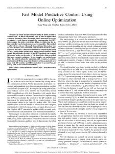
4.1 Example #1 The first example is a stable system with m = 3 inputs, p = 2 outputs and n = 12 states, in which the sampling time is 1 sec and the normalized inputs must satisfy the constraints: −1 ≤ uk ≤ 1. The MPC regulator is designed with the following parameters: N = 100, Q = C0C, R = 0.01Im , and thus the possible different active sets are 3200 = 2.656 × 1095 . Several partial enumeration solvers are compared: PE1, PE25, PE50, PE100 and PE200 use an active-set table with Ne = 1, 25, 50, 100 and 200 entries, respectively. As a comparison another solver is also considered: SH always computes and injects the optimal solution of (6) with a short control horizon of N¯ = 3. The different solvers are compared in a 20,000 decision timepoints simulation featuring 20 random step disturbances acting on the states, 20 random setpoint changes and normally distributed output noise. Table 1 provides the performance indices achieved by each solver. From this table it is evident that the use of a short control horizon can cause severe performance degradation while partial enumeration allows a fast computation of the optimal solution most of the times, with a small overall performance degradation. Figure 1 presents the cumulative frequency versus the number of entries scanned in the table by each partial enumeration solver. Figure 2 describes of the evolution of the active-set table for PE25 during the simulation, quantified by the folD(k,k−Ne ) lowing indices: Rd (k, 0) = D(k,0) , Ne , Rd (k, k − Ne ) = Ne in which D(k, j) is the number of table entries at time k that are not in the table at time j, while Ne is the number of all entries in the table. Figure 2 shows that the active-set table changes over time to adjust to new disturbances and operating conditions. The effect of the delay in solving the MPC problem in Step 4 was investigated first by introducing an integer parameter tlag which inflates the time required for solution of the full MPC problem. Specifically, if it is necessary to perform Step 4 at time k, the solution is assumed to become available for insertion in the table at time kavail defined by kavail = k +tlag . Figure 3 presents the results of this study for Example #1, in the case in which the table contains 25 entries. Note that, even for the small number of table entries, the suboptimality index SI remains close to its optimal value of 0 for tlag up to 50 and within a factor of one at tlag = 200. For tlag = 5000, the performance is as poor as the short-horizon backup strategy. In a second x-axis at the top of Figure 3, we quantify the effect of a computational delay differently. Consider the ratio of the the time it takes to solve the full MPC problem to the sample time. We define a parameter α, with which we inflate this ratio, so a solution computed at time k is available for insertion in the table at time kavail = k + αTQP (k)/TS . As displayed in Figure 3, the control performance loss is not significant until the full MPC calculation runs about 1000 times slower (or the sample time is 1000 times faster). 4.2 Example # 2: Crude Distillation Unit The second example is a crude distillation unit model with m = 32 inputs, p = 90 outputs and n = 252 states. Inputs and outputs are normalized, and the inputs must satisfy bound constraints. Only four outputs, representing the qual-

(25)

Moreover, WN (bs ) is positively invariant for the system w¯ j+1 = Aw¯ j + Bv¯ j with v¯ j defined as the first component of the control sequence solution of (5). We now describe conditions under which the initial deviation state w0 lies in WN (bs ), for all N sufficiently large. Theorem 3 Suppose the assumptions of Lemma 1 hold. Assume that for the current deviation state w0 there are state and input infinite sequences {w j } and {v j } that satisfy (5b) and (5c) (in which these constraints hold for all j) and such that the corresponding objective function in (18) is finite. Then, there exists a finite integer N 0 (which depends on w0 ) such that w0 ∈ WN (bs ) for all N ≥ N 0 . (26) Finally, we describe a nominal stability property for Algorithm 1. Theorem 4 The control input uk computed from Algorithm 1 is feasible with respect to (2) for any current deviation state w0 and target bs . Moreover, under the assumptions of Lemma 2, the outlined procedure is closed-loop nominally stabilizing, that is, (w j , v j ) → 0 for any w0 ∈ WN (bs ). 4

Application examples Two examples are examined to evaluate the proposed partial enumeration algorithm and compare it with a commercial active-set solver, qpsol. All simulations are performed using Octave on a 1.2 GHz PC, and time is measured with the function cputime [more details can be found in (Pannocchia et al., 2006)]. Partial enumeration solvers are implemented, for backup calculation of a suboptimal input, with δmax = 0.0001 and short control horizon of N¯ = 3. The following performance indices are considered. N • Optimality rate: OR := Nopt , in which Nopt is the number tot of decision timepoints in which the optimal solution was found in the table and Ntot is the overall number of decision timepoints. ∗| • Suboptimality index: SI := |Φ−Φ Φ∗ , in which Φ is the achieved closed-loop objective function and Φ∗ is the optimal one. T∗ ∗ and T • Average speed factor: ASF := Taver , in which Taver aver aver are the average times required to compute the optimal and the (sub)optimal input. ∗ ∗ and • Worst-case speed factor: WSF := TTmax , in which Tmax max Tmax are the maximum times required to compute the optimal and the (sub)optimal input.

6

of all disturbance scenarios expected in normal plant operation. In this work two backup strategies are presented for use when the optimal control is not in the current table: a restriction of the previous, optimal trajectory, or a short control horizon solution. One can readily imagine other backup strategies that may prove useful in practice. Of course, a complete solution for large-scale problems remains a challenge. The PE method pushes back the current boundary between what size application is and is not tractable using MPC.

ity of the crude distillation unit side products, have desired setpoints, and the MPC regulator is designed with the following parameters: N = 25, Q = C0C, R = 20Im . The number of possible different active sets is 3800 = 4.977 × 10381 . Response of the “true” plant is simulated by adding, to the nominal model response, unmeasured random step disturbances on the crude composition, on the fuel gas quality and on the steam header pressure, and normally distributed output noise. Five partial enumeration solvers are compared: PE1, PE25, PE50, PE100, PE200 use an active-set table of 1, 25, 50, 100 and 200 entries, respectively. The different solvers are compared on a 5 day (7201 decision timepoints) simulation with 10 random disturbances and 5 setpoint changes. Table 1 provides the performance indices obtained with each solver. Table 1 shows that the partial enumeration solvers provide low suboptimality with remarkable speed factors, especially when small tables are used. This largescale example is particularly challenging since on average qpsol takes about 26 seconds to compute the optimal input with a worst-case of about 53 seconds. In comparison, PE25 requires in the worst-case about 1.3 seconds, and is therefore definitely applicable for real-time implementation with sampling time of 1 minute. Active constraints are the rule in this example. On average, about 9 inputs (out of 32) are saturated at their (lower or upper) bound at each sample. The fully unconstrained solution (LQ regulator) is not feasible at any sample time in the simulation. The crude distillation unit operation under MPC control is always on the boundary of the feasible region, which is expected to be typical of large-scale, multivariable plants.

Acknowledgments The authors would like to acknowledge Dr. Thomas A. Badgwell of Aspen Technology, Inc. for providing us with the crude distillation unit model. References Bartlett, R. A., Biegler, L. T., Backstrom, J. & Gopal, V. (2002). Quadratic programming algorithms for large-scale model predictive control. Journal of Process Control, 12(7), 775–795. Bemporad, A., Morari, M., Dua, V. & Pistikopoulos, E. N. (2002). The explicit linear quadratic regulator for constrained systems. Automatica, 38, 3–20. Cannon, M., Kouvaritakis, B. & Rossiter, J. A. (2001). Efficient active set optimization in triple mode MPC. IEEE Transactions on Automatic Control, 46(8), 1307–1312. Chisci, L. & Zappa, G. (1999). Fast QP algorithms for predictive control. in ‘Proceedings of the 38th IEEE Conference on Decision and Control’. Vol. 5. pp. 4589–4594. Johansen, T. & Grancharova, A. (2003). Approximate explicit constrained linear model predictive control via orthogonal search tree. IEEE Transactions on Automatic Control, 48(5), 810–815. Kouvaritakis, B., Cannon, M. & Rossiter, J. A. (2002). Who needs QP for linear MPC anyway. Automatica, 38, 879–884.

5

Conclusions Partial enumeration (PE) has been presented as a method for addressing large-scale, linear MPC applications that cannot be treated with current MPC methods. Depending on the problem size and sampling time, online QP methods may be too slow, and offline feedback storage methods cannot even store the full feedback control law. The PE method was shown to have reasonable nominal theoretical properties, such as closed-loop stability. But the important feature of the method is its ability to handle large applications. The industrial distillation large example presented demonstrates suboptimality of less than 0.01%, with average speedup factors in the range of 83–220, and worst case speedups in the range of 4.8–39.2. Small tables with only 25–200 entries were used to obtain this performance. These small tables contain the optimal solution at least 75% of the time given an industrially relevant set of disturbances, noise, and setpoint changes. Many extensions of these basic ideas are possible. If one has access to several processors, the storage table can be larger and hashed so that different CPUs search different parts of the table. Several CPUs also enable one to calculate more quickly the optimal controls missing from the current table. One can envision a host of strategies for populating the initial table depending on the user’s background and experience, ranging from an empty table in which all table entries come from online operation, to more exhaustive simulation

Kouvaritakis, B., Rossiter, J. A. & Schuurmans, J. (2000). Efficient robust predictive control. IEEE Transactions on Automatic Control, 45(8), 1545–1549. Lie, B., Diez, M. D. & Hauge, T. A. (2005). A comparison of implementation strategies for MPC. Modeling Identification and Control, 26(1), 39–50. Mayne, D. Q., Rawlings, J. B., Rao, C. V. & Scokaert, P. O. M. (2000). Constrained model predictive control: Stability and optimality. Automatica, 36(6), 789–814. Milman, R. & Davison, E. J. (2003a). Evaluation of a new algorithm for model predictive control based on non-feasible search directions using premature termination. in ‘Proceedings of the 42nd IEEE Conference on Decision and Control’. pp. 2216–2221. Milman, R. & Davison, E. J. (2003b). Fast computation of the quadratic programming subproblem in model predictive control. in ‘Proceedings of the American Control Conference’. pp. 4723–4729. Muske, K. R. & Rawlings, J. B. (1993). Model predictive control with linear models. AIChE Journal, 39, 262–287. Pannocchia, G. & Rawlings, J. B. (2003). Disturbance models for offsetfree model predictive control. AIChE Journal, 49, 426–437. Pannocchia, G., Rawlings, J. B. & Wright, S. J. (2006). ‘The partial enumeration method for model predictive control: Algorithm and examples’. TWMCC-2006-01. Available at http://jbrwww.che.wisc. edu/jbr-group/tech-reports/twmcc-2006-01.pdf. Rao, C. V., Wright, S. J. & Rawlings, J. B. (1998). Application of interiorpoint methods to model predictive control. Journal of Optimization Theory and Applications, 99, 723–757.

7

Rojas, O., Goodwin, G. C., Ser´on, M. M. & Feuer, A. (2004). An SVD based strategy for receding horizon control of input constrained linear systems. International Journal of Robust and Nonlinear Control, 14(13-14), 1207–1226.

0.894

Cumulative frequency

0.893

Seron, M. M., Goodwin, G. C. & De Don´a, J. A. (2003). Characterisation of receding horizon control for constrained linear systems. Asian Journal of Control, 5(2), 271–286. Tondel, P., Johansen, T. A. & Bemporad, A. (2003). An algorithm for multi-parametric quadratic programming and explicit MPC solutions. Automatica, 39, 489–497.

0.892 0.891 0.89 0.889

Table 1 Performance indices for the examples. SI

ASF

WSF

OR

SI

ASF

0

50

WSF

SH

–

6.083

523

240

PE1

0.888

0.0580

302

230

0.654

6.9 · 10−5

610

399

PE25

0.890

0.0537

225

46.0

0.752

6.8 · 10−5

220

39.2

PE50

0.891

0.0537

181

20.9

0.762

6.8 · 10−5

162

20.1

PE100

0.892

0.0537

135

17.8

0.770

6.8 · 10−5

121

10.1

PE200

0.894

0.0537

89.6

14.4

0.786

6.8 · 10−5

83.3

4.79

100

150

200

Number of entries scanned

Fig. 1. Example # 1: cumulative frequency of finding an optimal entry versus number of entries scanned. Most of the benefit is achieved with small tables, and then optimality increases only slowly with table size. 1 0.8 0.6 0.4 0.2 0

Rd (k, 0)

OR

0.887

Example #2

0

5000

10000 Time (min)

15000

20000

0

5000

10000 Time (min)

15000

20000

1 0.8 0.6 0.4 0.2 0

Rd (k, k − Ne )

Example #1

PE50 PE100 PE200

0.888

Fig. 2. Example #1: table relative differences for PE25. The top figure shows that the original table is completely replaced as plant operation evolves. The bottom figure shows that the table turns over quickly during some periods and remains fairly constant during other periods. α 102

103

104

105

7 6

short horizon

5 4 SI

PE 3 2 1 optimal

0 1

101

102 tlag

103

104

Fig. 3. Example #1: suboptimality versus computational delay. For a wide range of the computational delay, partial enumeration provides almost optimal performance.

8