FAST LCD MOTION DEBLURRING BY DECIMATION AND OPTIMIZATION. Stanley H. Chan and Truong Q. Nguyen. ECE Dept, UCSD, La Jolla, CA 92093-0407.
FAST LCD MOTION DEBLURRING BY DECIMATION AND OPTIMIZATION Stanley H. Chan and Truong Q. Nguyen ECE Dept, UCSD, La Jolla, CA 92093-0407 http://videoprocessing.ucsd.edu ABSTRACT The LCD deblurring problem is considered as a simple bounded quadratic programming problem and is solved using conjugate gradient with early stopping criteria to avoid excessive search. A decimation and interlace interpolation method is introduced to reduce the computing time. Solutions are competitive to those the generated by conventional Lucy Richardson algorithm, but using much shorter amount of time. The method can be extended to higher decimation factors. Visual subjective tests are conducted to justify our proposed method. Index Terms— LCD, motion blur, inverse problem, optimization, decimation.
1. INTRODUCTION Liquid Crystal Display (LCD) differs from traditional cathode ray tube (CRT) display by its sample and hold behavior versus the CRT’s impulse driven behavior. Such sample and hold behaviors cause motion blur in video. In [1], Har-Nor et al demonstrated a novel signal processing strategy to preprocess the video signal such that the video sequence is oversharpened. When it is subjected to the motion blur, the output would be close to the target video. The main algorithm that Har-Nor et al applied is standard Lucy Richardson (LR) algorithm [2] (using MATLAB routine deconvlucy). Though the results are satisfactory, the computing time is long. In this paper, we propose a new approach that reduces the computational time significantly while retaining visual performance. We consider the problem as an optimization problem. First, as in most classical deblurring algorithms we are going to assume linear shift invariant image system. Thus for an m × n image x, and a point spread function (PSF) h, the output would be given by y = h⋆ x, where ⋆ denotes a convolution operator. In linear algebra words, if we stack columns of x as an mn × 1 vector, and let A be the convolution matrix, then given the target b ∈ Rmn×1 we would like to solve the This project is supported by AMD and UC Discovery.
following optimization problem: minimize kAx − bk22 mn
(1)
0 ≤ x ≤ 1.
(2)
x∈R
subject to
The simple bound constraint 0 ≤ x ≤ 1 is posed to limit the magnitude of the pixels to not exceeding 1 and 0. This quadratic programming problem is difficult because it has a huge number of variables (medium sized image with 1000 × 1000 pixels will have 1 million variables). Therefore a good algorithm for this problem 1. should be fast; 2. does not need to store matrices A, and AT ; 3. can give visually satisfactory results (not only PSNR). Based on these criteria, we propose to down sample the images and then apply conjugate gradient algorithm for the constrained optimization. The solution will be reconstructed using an interlace interpolation method. The image quality by the proposed method is as good as the one generated by LR, but using significantly shorter time. The organization of this paper is as follows. In section 2 we will describe the main blocks of our algorithm. In section 3 we will extend the factor to arbitrary integers. Some experimental results are shown in section 4, and a concluding remark will be given in Section 5. 2. INTERLACE INTERPOLATION 2.1. Overall system Human eyes pay much more attention to horizontal motions than vertical motions. Therefore, in this paper we assume that the PSF is horizontal (if not, we can approximate the PSF with a separable PSF and take its x-component). Then, since the rows are independently convolved, we can treat one row at a time. Also, since adjacent frames of a video are highly correlated, it is possible to consider only a few rows of the current frame, and reconstruct the remaining from its adjacent frames. Fig. 1 shows the block diagram to compute one frame. For the k th (k is even) frame Ik , the image is first down sampled and only the even rows are taken. Denote it by (Ik )even . Then (Ik )even is passed into conjugate gradient algorithm to
(Ibk )even (Ik+1 )odd Ik+1
↓2
CG
(Ibk+1 )odd
(Ibk−1 )odd
Reconstruction
(Ibk )f ull
Fig. 1. Block diagram of our proposed fast inverse computation. We inverse compute the desired image for (Ik+1 )odd , and use previous information (Ik−1 )odd and (Ik )even to reconstruct the current frame (Ik )f ull . When proceeding to the next frame, we swap the odd and even indices. obtain the inverse solution (Ibk )even . The subscript even is used to emphasize that (Ibk )even has only half number of rows as Ibk (to be determined). If k is odd, the roles of even and odd in the above will be swaped. Suppose the current solution to be reconstructed is Ik . From previous iterations the full size solution (Ibk−1 )f ull can be obtained. Since previously when (Ibk−1 )f ull was reconstructed the k th inverse solution (Ibk )even had already been computed, in the k th frame reconstruction there is not need to re-compute it again. However, the k + 1th inverse solution to reconstruct (Ibk )f ull is needed. Therefore, we apply conjugate gradient to the decimated image (Ik+1 )odd and obtain the inverse solution (Ibk+1 )odd . Then the three decimated inverse solutions {(Ibk−1 )odd , (Ibk )even , (Ibk+1 )odd } are passed to the reconstruction scheme and the k th reconstructed image can be obtained. 2.2. Interlace Interpolation The interlace interpolation method is shown in Fig. 2. Having the inverse solution (Ibk−1 )odd , (Ibk )even , and (Ibk+1 )odd , we would like to fill in the unknown rows of (Ibk )even . First assume that the frames are motion compensated (using linear motion compensation) and aligned on the same pixel. Consider the corresponding pixels of the k − 1th frame and the k + 1th frame, the upper and lower pixel of the k th frame. The solution can be estimated as (Ibk )f ull (m, n) = 0.4(Ibk−1 )odd (m, n) + 0.4(Ibk+1 )odd (m, n)
+ 0.1(Ibk )even (m, n + 1) + 0.1(Ibk )even (m, n − 1).
Note that this is a weighted sum of the four corresponding pixels, where the weights are empirically justified. 2.3. Conjugate Gradient The main algorithm in this paper is conjugate gradient. It can be summarized as [3]:
(Ibk−1 )odd
(Ibk )even
(Ibk+1 )odd
Fig. 2. Proposed linear interpolation method. To distinguish the known pixels from the unknown pixels we shaded the known ones. We take weighted mean of the corresponding pixels from previous frame (Ibk−1 )odd (m, n), next frame (Ibk+1 )odd (m, n), upper pixel Ibk even (m, n + 1) and lower pixel Ibk even (m, n − 1). Here we assume that the previous and the next frames are motion compensated. Initial Condition Given x0 , set r0 ← Ax0 − b, p0 ← −r0 , k ← 0 While rk 6= 0 xk+1
← ←
x
=
rk+1
←
βk+1 pk+1 k
← ← ←
αk
T rk rk pT k Apk
x (k + αk pk 1 x>1 0 x= 10, or, obj_val