Fast Linear Transformations in Python

Fast Linear Transformations in Python Christoph Wagner, Sebastian Semper October 27, 2017

arXiv:1710.09578v1 [cs.MS] 26 Oct 2017

Abstract

students. In fact, the vast majority of literature on signal processing methods relies on linear models, often found by approximating the underlying physical phenomenon by this more tractable model.

This paper introduces a new free library for the Python programming language, which provides a collection of structured linear transforms, that are not represented In engineering besides the pure mathematical investias explicit two dimensional arrays but in a more effi- gations also numerical simulations play an increasingly cient way by exploiting the structural knowledge. crucial role during research. Their purposes are manifold, in this case they range from demonstration to veriThis allows fast and memory savy forward and back- fication, numerical assessment to estimate performance ward transformations while also provding a clean but or complexity over to parameter tuning involved in varstill flexible interface to these effcient algorithms, thus ious algorithms. Very often these simulations deal with making code more readable, scable and adaptable. linear systems of the form as in (1), where for instance either x or y are unknown and have to be computed We first outline the goals of this library, then how they for fixed AL . were achieved and lastly we demonstrate the performance compared to current state of the art packages Additionally, a lot of problems in engineering and sigavailable for Python. nal processing are infinite dimensional by nature. With the growing power of computers the achievable resoThis library is released and distributed under a free lution in simulating these problems increases as well, license. where the size of the problem often is determined by some temporal or spatial resolution of the underlying physical problem. Hence, to get a better finite dimensional approximation when analyzing a problem the 1 Introduction computational complexity has to increase as well. To this end the physical computing power of computer is increasing as well in terms of speed and memory size. 1.1 Motivation However, some problems like three dimensional X-Ray tomography are easily exceeding the processing power of any computer if one only wants to calculate y from x in (1), because the entries of y obey the formula of the matrix-vector product as in (1), which explicitly reads as m X yi = ai,k · xk for i = 1, . . . , n, (2)

Linearity is a mathematical concept that reaches into almost all branches of science, where on the one hand many models identify the objects they are dealing with with elements a vector space, i.e. a linear space, where on the other hand the transforms that preserve this linear structure are called linear transforms. When dealing with such a linear mapping L between two finite dimensional vector spaces V to U over a complex or real valued field one often describes this mapping in coordinates as a map from Rm to Rn or from Cm to Cn respectively using a matrix AL ∈ Cn×m via x 7→ AL · x = y,

k=1

where the ai,j are the entries of the matrix AL . This reveals that calculating all entries of y has time complexity O(n · m) and storing AL also has space complexity O(n · m). In case of n = m they both scale quadratically with the dimension of x. At first sight this might seem efficient enough, but problems where AL does not fit into system memory often occur for example in image processing. For instance, consider a filtering operation applied to an image, where a typical image size of current consumer grade cameras is 20 MP. These are represented by vectors that contain 20 · 220 pixel values in the case of an 20 MP image. Since some filtering operations are linear and as such they can be

(1)

where m and n are the dimensions of U and V respectively and x and y are vectors in Cm and Cn . All properties of the linear mapping L transfer to properties of AL . Because of their importance in science and engineering they have been studied intensively during the past decades and are well understood and an elementary concept in the curriculum of undergraduate 1

1.2

Structured Linear Mappings

1 INTRODUCTION

conveniently expressed as A · x = y. However, the corresponding matrix would contain 400·240 entries, which is impossible to store on most systems, since it would need ≈ 1.8 Petabytes of storage if the entries where represented with 32 Bit variables. Still, we are able to calculate these linear filters within a very short amount of time. Even small chips integrated in digital cameras can apply simple filters to the images they capture. But in this case they do not use the general formulas in (1) and (2). Instead, they use algorithms specifically tailored to the structural information available. This tailoring process mostly drops the association of the linear mapping with a matrix and only exposes a routine to calculate the matrix vector product. The mathematical notation in scientific publications on the other hand still maintains this matrix and vector formalism, which preserves all the possible algebraic interactions among matrices and vectors. Hence it would be advantageous if one had this freedom in formalism at hand when writing code to make the transition between theoretical derivations and efficient implementations easier.

1.2

for Fourier Transforms, convolutions, Wavelets, Shearlets [11], Curvelets [15] and many more, which aim to provide good performance while hiding all implementational complexity from the user beneath an abstraction layer. Since it has become clear in the recent years that by exploiting structure in linear transforms one can alleviate the bottleneck of the standard matrix-vector product [6]. There has been a surge of interest in developing numerical algorithms that only make use of these forward and backward transforms when calculating other properties of a linear mapping, like eigenvectors, eigenvalues, or solutions to linear systems. Together with the above-mentioned specific libraries one can apply these algorithms to specific problems and make them feasible by exploiting their inherent structure.

1.3

The Problem of Abstraction

As already mentioned, these specific algorithms for efficiently applying a matrix to a vector need an abstraction layer that makes them usable for a broad scientific audience. Unfortunately these abstractions obey a different design for different libraries used. This introduces different kinds of problems during the usage of these libraries. First, the interoperability between those libraries is often hard to realize, when one encounters a specific problem that needs to make use of several libraries at once. Second these libraries are often used in a counterintuitive way, because the actual programming code diverges a lot from the mathematical expressions that describe the problem at hand in the corresponding publication. This makes the code hard to read and debug, because the identification between code and mathematical notation gets obfuscated by technical necessities. Moreover, it creates an obstacle for third party scientists in understanding the method presented in some publication. Last, when manually stitching various libraries together into one huge conglomerate, it makes this development mainly unusable for any future project because of its adaption to a specific task at hand. This sparks the need for a uniform abstraction layer, which enables the interoperability between various efficient libraries together, thus creating a uniform interface to work with.

Structured Linear Mappings

Most of the linear mappings that one encounters in applications obey a certain structure and it can yield a significant gain in computation speed and memory efficiency if one does so. In case of a linear image filter this could be the convolution y = c ∗ x, where AL then would be a circulant matrix. This structure allows to derive more efficient means of storing AL and also calculating AL · x. However, these algorithms do not use shortcuts to lower (2) explicitly but take mathematical
the complexity from O n2 to O(n log n). The maybe most famous example for an algorithm of this type is the Fast Fourier Transform (FFT), which efficiently applies the discrete Fourier Transform to a vector, where AL = F is the Fourier matrix. In this case there are efficient methods to calculate F · x and F H · x, where the first one is the so called forward transform and the latter is called backward transform. In case of the FFT one does not need to store F leading to no storage consumption at all. In other words the FFT is a so called matrix-free algorithm. It should be noted that a low complexity algorithm, which might not be implemented very efficiently will outperform a highly optimized algorithm with a theoretically higher memory or time complexity as soon as the problem size surpasses a certain threshold. So although there are many very efficient BLAS libraries, which try to be as efficient as possible they often are only able to encompass very high level structural information into their calculations, like symmetry of the respective transform or positive definiteness.

1.4

Development Goals

Considering everything from above, i.e. the large problem size, the specific algorithms and the need for abstraction, led the authors to the development of a library that encompasses all of the above desired features while spanning an easy to use interface to the Nowadays there are a lot of specific libraries that are increasingly popular programming language Python. dedicated to specific linear transforms for a wide va- This library is called fastmat and it is the subject of riety of programming languages. There are packages the following chapters. 2

1.5

Relation to other Software

3

The first goal is to provide many efficient implementations for various types of structures to make fastmat relevant for as many applications as possible. Second the transition of already existing code from own implementations to this new library should be as easy and simple as possible. This should be realized by an efficient and lean interface to other standard scientific computing libraries already present in Python. This leads to the third goal, that the usage should be intuitive to users familiar with the programming language, which in the community is referred to as being “pythonic”. Next its performance should be transparent to the user, which means that one should be able to directly measure or estimate the performance of fastmat on a given machine in comparison to other software packages to provide a direct criterion for determining the effect of a possible adaption to any code already or soon to be existing. Moreover a high degree of modularity should allow the future extension by new transforms or general features. Last but not least, the library should be available under a free license in order to minimize any financial or structural hurdles in testing and using fastmat.

USE CASES

subroutines. This sparks the possibility to also incorporate fastmat nodes into this calculation graph, where inputs and outputs of these nodes would be vectors before and after a certain linear transformation. There is a Matlab [17] package, called Spot [2], which introduces abstract linear operators for this proprietary software that is uniformly present in natural sciences and engineering. Unfortunately it seems like it is no longer actively developed. And although the package itself is distributed under a free license, it obviously depends on Matlab, which is not freely available and as such introduces an additional financial hurdle.

2

Architecture

First, it provides a collections of efficiently implemented algorithms for the calculation of M · x and M H · x for some specifically structured matrix M ∈ Cn×m , i.e. the already introduced forward and backward transforms. Here, fastmat in some cases only provides a consistent wrapper around routines already 1.5 Relation to other Software included in numpy and scipy, which are by now well documented and adapted libraries for scientific computing First one should mention the two packages numpy and present in Python. These wrapped routines are for exscipy [16] as crucial building blocks in fastmat, because ample the FFT or the implementation of various sparse it adapts the data structures and data types from these matrices. two widely adopted libraries within the Python community. The reason behind this is that it saves precious development time which can then be focused on Use Cases the transforms’ algorithms instead. Also, the two men- 3 tioned packages are very well designed, tested, maintained and mature, which makes them solid founda3.1 Low System Memory tions to rely on during development. In [6] the authors describe a framework for convex optimization, which allow to describe an optimization problem not with the matrices themselves but only with functions that realize the forward and backward transforms of the involved matrices. Their motivation is a similar one as the one behind fastmat, since they are able to exploit efficient implementations that way during optimization. These routines needed there are exactly those which are also provided by the proposed library. This means both projects can easily be combined and complement each other.

In traditional scientific computing tools, like [17] or [16], the matrices the user works with have to be stored in memory in order to be applied to a vector or to solve a system of linear equations. If the dimension of the involved vectors is large, the memory needed to store the appropriate matrices scales quadratically with the problem size. So the system memory might get depleted very soon. However, when using fastmat the structural information about the matrices makes sure that only the quantities needed to carry out the forward and backward transform are stored.

A recent publication [19] goes one step further and proposes to describe complex calculations in an optimization framework with a so called calculation graph, where single nodes of that graph represent mathematical operations like addition, subtraction or whole linear transforms. This allows a high flexibility in the choice of tools used to carry out a specific task. If for example a certain task is highly parallelizable, this certain node can invoke a calculation on a GPU, whereas other tasks can be performed by standard BLAS or LAPACK

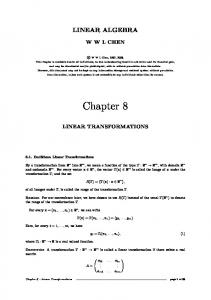
The Kronecker product is a good example to illustrate the effect of explicitly storing matrices. Because for A ∈ Cn×m and B ∈ Ck×ℓ the Kronecker product A ⊗ B is in Cn·k×m·ℓ . So even if A and B fit into the system memory, their Kronecker Product may not. In Figure 3 we measured the memory used by M = F ⊗ D ⊗ A, where F ∈ Ck×k is a Fourier matrix, D ∈ Ck×k is a diagonal matrix and A ∈ Ck×k is a dense unstructured matrix, which yields n = k 3 and 3

3.1

Low System Memory

3

Partial Transpose

Blocks Kronecker Product

Power

Polynomial

Block Diagonal Circulant

Product

Matrix

Parametric

Toeplitz

Hadamard Sparse Identity Diagonal

Fourier

Zero

Figure 1: Class dependencies in

Matrix

fastmat

Hadamard

forward():

forward():

• user entry point • check dimensions • check types • consistency • interfacing

• inherited from Matrix

numN

numN

__forward(): • hidden from user • efficient calculation

• N - dimension

. . .

. . .

Figure 2: Inheritance scheme in

4

fastmat

USE CASES

3.2

Systems of Linear Equations

3

once or several times each iteration. Some well known examples are the method of Conjugate Gradients (cgmethod) [8] to solve a symmetric system of linear equations, its extension the Bi-Conjugate Gradients Stabilized [18] (BiCGStab) to the non-symmetric case, the Power Iteration to calculate eigenvalues and -vectors or its refinement the Arnoldi Iteration [9] or so called thresholding algorithms used for sparse recovery [1]. Two of these algorithms are presented in a concise form and used to compare the speed of fastmat to other libraries.

106 Kronecker Product

106 bytes

numpy dot fastmat

4

10

102

100 101

102

103

USE CASES

104

n

To illustrate the performance of the presented library to a universally important problem on many fields of Figure 3: Memory consumption of fastmat when stor- research, we want to solve a system of linear equations ing a Kronecker product compared to numpy. of the form A·X = Y, (3) 3

3

M ∈ Ck ×k . As we can see the memory consumption of numpy grows according to the dimension of the Kronecker product of the involved factors and scales like O(k 6 ), which rapidly exceeds any available memory for even modest problem sizes. This is due to the fact, that the whole Product has to be precomputed completely beforehand and all entries of the 2D array had to be held in memory. On the other hand, fastmat is designed to only store the factors of M , where the Fourier matrix needs constant storage, the diagonal matrix’ D storage takes up O(k) of memory and the memory footprint of A scales as O(k 2 ) making the whole storage consumption of the order O(k 2 ).

for A ∈ Cm×m , X ∈ Cm×k and Y ∈ Cm×k , where A obeys some structural constraint and being full rank, Y is known and we seek to calculate X. Formally we could write X = A−1 · Y , (4)

which would entail that we first calculate the n × m elements of A−1 and then apply it to Y . It is clear that this is highly inefficient in terms of memory and computation time. Instead we use the method of Conjugate Gradients. In the case where A is already symmetric (or hermitian in the complex case) already, we solve (3) and if not, we modify (3) to
AH A · X = AH · Y , (5) The code snippet in Listing 1 depicts the simplicity of the construction of a huge Kronecker product which although possibly harming the condition number of the needs basically no system memory, because the product system. there also is the possibility to use an algorithm is completely matrix free. that can also treat the non-symmetric case as depicted in [18]. # import the packages import fastmat

As described in [8], the iteration needs to apply the system matrix to a vector at each step, which turns out to be the most costly part of the algorithm. The rest of the operations consist of inner products and scalar multiplications of vectors. Since it is one of the algorithms, where fastmat performs best, this method is already tightly integrated into fastmat and readily available to the users.

# a 1024x1024 sized fourier matrix F = fastmat.Fourier(1024) # a 1024x1024 sized diagonal matrix D = fastmat.Diagonal(d) # a dense random matrix A = fastmat.Matrix() # a 1024^2 x 1024^2 sized kronecker product M = fastmat.Kron(F, D, A)

In Listing 2 one can see an example, where a circulant matrix with 240 elements is initialized and the CG algorithm is invoked. Solving (3) for x with a Circulant A is called deconvolution.

Listing 1: Code example that illuminates the construction of Kronecker products used in Figure 3.

3.2

# import the packages import numpy.random as npr import fastmat as fm import fastmat.algs as fma

Systems of Linear Equations

# create random right hand side y = npr.randn(2 ** 20)

Another case where fastmat performs most efficient are those, where only forward and backward transforms are necessary. Most of these algorithms are iterative ones, which make use of the matrix-vector product

# convolution vector c = npr.choice([-1, 1], 2 ** 20, replace = 1)

5

3.3

Sparse Recovery

3

USE CASES

which under certain assumptions can be solved via a solution to

# create the convolution matrix A = fm.Circulant(c)

(8)

min λkzk1 + kb − A · D · zk2 ,

# solve for x x = fma.CG(A, x)

z∈Cm

time[s]

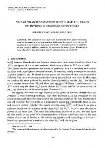
for appropriately chosen λ > 0. As a means of solving Listing 2: Code example that illuminates the usage of the above problem, one can consider so called iterathe CG algorithm. tive thresholding methods, which can be found together with analysis of above problems in [1]. Essentially these The above code illuminates how simple the interface to algorithms carry out the iteration the efficient algorithms is designed and how seamless
it interacts with common Python data structures. To (9) xk+1 = tc xk − αM H (b − M xk ) complete the presentation of the CG method we give a performance chart in Figure 4 which compares the until convergence, where in our case M = A·D, α > 0 proposed library to the solve routine present in numpy. is a step size and tc is the thresholding operator. The important fact here is that this iteration spends most of its computation time in calculating the forward and 10−1 Solving a LES backward projection of the matrix M . Moreover, in fastmat many application scenarios the basis D is highly strucnumpy 10−2 tured and has an efficient transformation. It could be a Fourier, Wavelet or Circulant matrix. Moreover, it has 10−3 been suggested to construct the compression matrix A by randomly selecting rows from again a Fourier or 10−4 Hadamard matrix [10]. This random selection can be handled by fastmat, while still preserving the fast algo10−5 rithm of the matrix the rows got selected from. In case of these constructions one can show, that the iteration 101 102 103 in (9) exactly recovers the original x. To demonstrate n Figure 4: Average performance of fastmat when solving a system of linear equations compared to numpy.

101

100 steps of ISTA fastmat

3.3

time[s]

100

Sparse Recovery

Sparse (Signal) Recovery (SSR) has been a rapidly growing field of interest in many branches of signal and antenna array processing, because together with Compressive Sensing (CS) it allows stable and robust recovery of heavily undersampled, or compressed, hence the name, signals under the condition, that the signal to recover obeys a sparsity condition [3, 4]. A common undersampling strategy is the one, which applies linear measurements to a signal y = D ·x, where D ∈ Cm×m is the so called sparsifying basis or dictionary, y ∈ Cm and x ∈ Cm is a sparse vector, i.e. it has only a few non-zero entries compared to its dimension. Since, the measurements are linear, we can express the whole SSR Model the following way b = A · y = A · D · x,

10−3 101

102

103

104

n

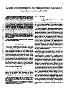
Figure 5: Speed comparison between numpy and when carrying out Sparse Signal Recovery.

fast-

mat

the effect on the reconstruction time when using structured matrices during the process, we carried out 100 of the Iterative Soft Thresholding Algorithm (ISTA) [1] and we compared the runtime of the exact same amount of steps when doing the standard forward and backward projections according to (2) with the functionality provided by numpy to the runtime, when using the algorithms provided by fastmat. Here D is a circulant matrix and A is a matrix with rows randomly selected from a Hadamard matrix. The results are depicted in Figure 5.

(6)

where A ∈ C is the measurement matrix with n ≪ m and b is the so called measurement vector. The goal is now, to recover x and hence y from b under the sparsity prior. First this seems impossible, because the linear system in (6) is highly underdetermined. But as it turns out [5] the optimization problem z∈C

10−1 10−2

n×m

minm kzk1 s.t. b = A · D · z,

numpy

As one can see fastmat outperforms numpy, while deliv(7) ering the exact same results at moderate problem sizes 6

3.4

Synthetic Aperture Focusing Technique

4

roughly by a factor of 100. With growing dimensions this gap would grow even larger until the point that numpy totally depleted the memory by storing A · D.

S_0 = fm.Sparse(...) S_p1 = fm.Sparse(...)

3.4

# define M row wise M = fm.Blocks( [S_n1, Z, Z, Z], [S_0 , S_n1, Z, Z], [S_p1, S_0, S_n1, Z], [Z , S_p1, S_0, S_n1], [Z , Z, S_p1, S_0], [Z , Z, Z, S_p1], )

COMPARISONS

# define a Zero matrix Z = fm.Zero(n, n)

Synthetic Aperture Focusing Technique

Synthetic Aperture Focusing Technique (SAFT) is a postprocessing method in non-destructive ultrasonic testing, which is used to focus measurements after acquisition. Based on a simplified physical forward model the reflectivity inside the tested specimen is visualized Listing 3: Code example which implements the matrix by a delay and sum strategy. In its most common form, M from equation (10) for K = 1. the focusing consists of summing the measured data along hyperbolas, where each of these hyperbolas inIn Listing 3 the construction of M according to (10) tersects only a few samples within data. is given for the case K = 1 and one can see, how the Moreover, the SAFT algorithm can be expressed in a pointers to the specific matrices are reused to build up concise way using a single matrix vector multiplication the matrix, which does not store any unnecessary infor[12], where the involved matrix is highly structured mation, because any building block Sj is defined once and sparse, i.e. is comprised of several sparse matrices, and its position within M is described by the definition which occur several times in the matrix. So the struc- of the fm.Blocks object. tural knowledge can be exploited twofold. First we can save memory by using data structures for sparse matrices and by defining a fastmat block matrix, where only 4 Comparisons object references to the appropriate sparse matrices are stored, to describe the desired structure. The following paragraphs provide some further perforMore explicitly, the SAFT matrix reads as mance charts, which compare the performance of lin  ear transforms represented as a numpy array against the S−K 0 ... 0 representation provided by fastmat. ..   .. ..  .  . S . −K     .. .. S+K . 0  . , M = (10) 4.1 Kronecker Products   ..  0  S . S +K −K    . ..  .. ..  .. . . In section 3.1 we already presented how efficiently fast.  mat is able to handle Kronecker products when it comes 0 ... 0 S+K to memory. But it also is capable of carrying out the where the S−K , . . . , S+k are sparse matrices and are application of a Kronecker product M = A ⊗ B more aligned in block Toeplitz structure. Clearly, to fully efficiently by adapting a method presented in [7]. It describe M one only needs to define the matrices Sj as is worth noting that the algorithm described there alwell as their positioning within M . Current computer ready yields a gain in efficiency if the involved matrialgebra systems only allow to specify the whole matrix ces are unstructured and matrix-vector multiplication M as a sparse data structure without the possibility to is done as in (2). But since we are capable of performexploit the redundancy within M . The algorithm itself ing these operations more efficiently as well the gain can be simply written as the forward transform of M as in performance is twofold. Using the same matrices x 7→ M · x. With increasing resolution desired during as in Figure 3 but now comparing computation time, reconstruction, the number of rows and columns of each we get results depicted in Figure 6. As one can see Sj grows, as well as the mangitude of K. So while even for very small problem sizes, where the size of the it might be possible to store the whole M in system whole product exceeds 100. At problem sizes around memory for modest problem sizes, this approach will 104 the speedup factor of fastmat over numpy is of the ultimately exhaust the whole memory, thus making it order 104 as well. Kronecker products are of genera unfeasible in practice. importance, when dealing with vectorized multidimenˆ on sional data. Because the 2D Fourier transform M import fastmat as fm n×n an image M ∈ R reads as # define the sparse matrices S_n1 = fm.Sparse(...)

ˆ ) = (F n ⊗ F n ) · vec(M ). vec(M 7

4.2 Hadamard Matrices

4

10−1 10−2

10−2

Hadamard Transform

Kronecker Product

fastmat

10−3

fastmat

10−3

time[s]

time[s]

COMPARISONS

10−4

numpy

10−4 10−5

10−5

10−6

10−6 101

102

103

101

104

102 n

103

n

Figure 6: Calculation time with necker product compared to numpy.

fastmat

of a Kro- Figure 7: Comparison of fastmat and multiplying with a Hadamard matrix.

numpy

when

Similar relations hold for other types of transforms, like where the Mi are matrices themselves. wavelets for instance, which makes fastmat capable of efficiently applying linear transforms on multidimen10−2 Block Diagonal Matrix sional data in a flexible manner as long as these transfastmat form factorize with respect to the dimension. −3

4.2

time[s]

10

Hadamard Matrices

numpy

10−4 10−5

Hadamard matrices only have entries in the set {−1, 1} and are orthogonal. They are highly structured and their multiplication with a vector only involves additions and subtractions of the vector’s elements. This is the key idea behind the Fast Hadamard Transform, which was implemented in fastmat. Even for large dimensions this transform is very efficient, where in contrast to that the traditional matrix-vector multiplication quickly exceeds the available memory capacity or computing time.

10−6 101

102

103

104

n

Figure 8: Comparison of fastmat and numpy when multiplying with a block diagonal matrix consisting of a Fourier matrix F ∈ Ck×k and a random diagonal matrix D ∈ Ck×k , which yields n = 2k.

This type of matrices are important in various application fields and recently have been discovered to be suitable measurement matrices in Compressed Sensing, where one randomly selects rows of a Hadamard matrix. These randomly constructed matrices then have suitable properties for this specific application additionally to the fact that they have a fast transform.

The lower calculation time depicted in Figure 8 is not only achieved by considering the large amount of entries equaling zero but also by preserving the fast transforms of the components Mi that are used to make up the block diagonal matrix A.

As one can see in Figure 7, across the whole range of problem sizes fastmat outperforms numpy and in the 4.4 Algorithms higher ranges this happens by a speedup factor of about 104 . Among the already mentioned algorithms, which are ISTA (see Figure 5) for sparse signal recovery and the CG-method (see Figure 4) for solving systems of linear 4.3 Block Diagonal Matrix equations, we provide the Orthogonal Matching Pursuit algorithm [13], which also is a popular choice in Another type of matrix which often occurs in practice sparse signal recovery. This algorithm can be sped up are block diagonal matrices of the form using fastmat, because it uses a correlation step of a   vector with a matrix during each iteration. If this maM1 trix is structured this step, which also is the most time   .. A= , consuming, can be implemented more efficiently, hence . speeding up the whole reconstruction process. Mk 8

REFERENCES

Moreover, fastmat also includes two simple iterative or related ones. Additionally, we aim at providing effischemes to calculate the largest eigen- or singular value cient multiplication with the inverse of matrices, either using the Power Iteration. by exploiting structural knowledge or by sovling the appropriate system of linear equations. At this early stage of development we focused on package design and well implemented transforms, but in the Secondly we aim at exploiting structural knowledge future we aim at providing a richer collection of ready even further. Since the user is able to explicitly conto use methods that are built around fastmat to make struct matrix expressions of the form it more useful right out of the box in applications. M = C 1 · C 2 = F H D1 F F H D2 F ,

5 5.1

Conclusion

where C1,2 are both circulant matrices and the second equality is the fastmat internal treatment of these, we could use this information to refactor M to

Discussion

M = F H DF , where D = D1 ·D2 , thus saving two Fourier transforms and one diagonal matrix multiplication. To this end, the authors aim at implementing a rule based optimization system to detect even more numerical shortcuts in the expressions a user makes use of.

Despite the improvemments in efficiency for some types of problems or algorithms fastmat also entails some drawback. For instance, algorithms which work with structured matrices but also need to access or change specific elements very often during execution might be slower than before after having been ported to fastmat. But since the package allows to mix structured and unstructured linear transforms while still preserving all structural information, it still can be advantageous in certain scenarios to exploit structure in a small part of the processing pipeline.

Moreover, it would be advantageous if we could make complexity estimations of certain calculations on a specific machine. This leads to the possibility to dynamically switch between the fast transforms provided by fastmat and the conventional matrix-vector multiplication provided by numpy. These complexity estimation could also facilitate the term optimizations already Another point worth noting is that the close matchmentioned in the last paragraph. ing between code and the mathematical expressions make fastmat a very suitable choice for demonstration Additionally, we would like to provide means of parpurposes in teaching, because it is easy for students allelization where fastmat is able to act on chunks of to identify specific lines of code with the theoretical given data simultaneously on several CPU cores. So inderivations. Moreover it allows rapid prototyping for stead of parallelizing the algorithms themselves, which homeworks and exercises and does away with a lot of should be considered a large amount of work, fastmat obfuscating programming overhead involved with stan- will focus on distributing the processing of given parts dard tasks in signal processing. of data, this way making it also scalable on large computation clusters with many cores.

5.2

Release

References

The fastmat package is made public under the permissive annd open apache License 2.01 on [14] thus making it easily accessible, shareable and modifable. to the best of our knowledge it currently works on GNU/Linux and other proprietary Operating Systems.

5.3

[1] Amir Beck and Marc Teboulle. “A Fast Iterative Shrinkage-Thresholding Algorithm for Linear Inverse Problems”. In: SIAM Journal on Imaging Sciences 2.1 (Jan. 2009), pp. 183–202. issn: 1936-4954. doi: 10.1137/080716542. url: http://dx.doi.org/10.1137/080716542 (cit. on pp. 5, 6).

Further Development

[2] Ewout van den Berg and Michael P. Friedlander. Spot – A Linear-Operator Toolbox. url: http://www.cs.ubc.ca/labs/scl/spot/index.html (cit. on p. 3).

As development continues the authors aim at including more types of structured matrices to make the package more relevant in other areas of research. Such are for example outer products (tensor products), columnwise Kronecker products, Vandermonde matrices and some transforms localized in space and time, like Wavelets 1 https://www.apache.org/licenses/LICENSE-2.0

9

REFERENCES

REFERENCES

[3] E. J. Candes, J. Romberg, and T. Tao. “Ro- [12] Fredrik Lingvall, Tomas Olofsson, and Tadeusz bust uncertainty principles: exact signal reconStepinski. “Synthetic aperture imaging using struction from highly incomplete frequency insources with finite aperture: Deconvolution of the spatial impulse response”. In: The Journal of formation”. In: IEEE Transactions on Informathe Acoustical Society of America 114.1 (2003), tion Theory 52.2 (2006), pp. 489–509. issn: 0018pp. 225–234. doi: 10.1121/1.1575746. eprint: 9448. doi: 10.1109/TIT.2005.862083 (cit. http://dx.doi.org/10.1121/1.1575746. on p. 6). url: http://dx.doi.org/10.1121/1.1575746 [4] E. J. Candes and T. Tao. “Near-Optimal Signal (cit. on p. 7). Recovery From Random Projections: Universal Encoding Strategies?” In: IEEE Trans. Inf. [13] Orthogonal matching pursuit: recursive function approximation with applications to Theor. 52.12 (2006), pp. 5406–5425. issn: 0018wavelet decomposition. 1993, 40–44 vol.1. 9448. doi: 10.1109/TIT.2006.885507. url: http://dx.doi.org/10.1109/TIT.2006.885507doi: 10.1109/acssc.1993.342465. url: (cit. on p. 6). http://dx.doi.org/10.1109/acssc.1993.342465 (cit. on p. 9). [5] Scott Shaobing Chen, David L. Donoho, and C. Semper S. fastmat. Michael A. Saunders. “Atomic Decomposi- [14] Wagner https://github.com/EMS-TU-Ilmenau/fastmat. tion by Basis Pursuit”. In: SIAM Rev. 43.1 2017 (cit. on p. 9). (Jan. 2001), pp. 129–159. issn: 0036-1445. doi: 10.1137/S003614450037906X. url: [15] Jean-Luc Starck, E. J. Candes, and D. L. Donoho. http://dx.doi.org/10.1137/S003614450037906X “The curvelet transform for image denoising”. (cit. on p. 6). In: IEEE Transactions on Image Processing 11.6 (2002), pp. 670–684. issn: 1057-7149. doi: [6] Steven Diamond and Stephen Boyd. Matrix10.1109/TIP.2002.1014998 (cit. on p. 2). Free Convex Optimization Modeling. 2015. arXiv: 1506.00760 (cit. on pp. 2, 3). [16] S. Chris Colbert Stéfan van der Walt and Gaël [7] Paulo Fernandes, Brigitte Plateau, and William Varoquaux. “The NumPy Array: A Structure for J. Stewart. “Efficient Descriptor-Vector MultiEfficient Numerical Computation”. In: Computplications in Stochastic Automata Networks.” ing in Science and Engineering 13 (2011) (cit. on In: J. ACM 45.3 (1998), pp. 381–414. url: p. 3). http://dblp.uni-trier.de/db/journals/jacm/jacm45.html#FernandesPS98 [17] Inc. The MathWorks. MATLAB and Statistics (cit. on p. 7). Toolbox Release 2012b. Natick, Massachusetts, [8] Magnus R. Hestenes and Eduard Stiefel. “MethUnited States (cit. on p. 3). ods of Conjugate Gradients for Solving Linear [18] H. A. van der Vorst. “Bi-CGSTAB: A Fast Systems”. In: Journal of Research of the National and Smoothly Converging Variant of Bi-CG Bureau of Standards 49.6 (Dec. 1952), pp. 409– for the Solution of Nonsymmetric Linear 436 (cit. on p. 5). Systems”. In: SIAM Journal on Scientific and Statistical Computing 13.2 (1992), [9] Zhongxiao Jia. “The refined harmonic Arnoldi pp. 631–644. doi: 10.1137/0913035. url: method and an implicitly restarted refined algohttp://link.aip.org/link/?SCE/13/631/1 rithm for computing interior eigenpairs of large (cit. on p. 5). matrices”. In: Applied Numerical Mathematics 42.4 (2002), pp. 489–512. issn: 0168-9274. doi: [19] Matt Wytock et al. A New Architecture for Ophttp://dx.doi.org/10.1016/S0168-9274(01)00132-5. timization Modeling Frameworks. 2016. arXiv: url: http://www.sciencedirect.com/science/article/pii/S0168927401001325 1609.03488 (cit. on p. 3). (cit. on p. 5). [10] Felix Krahmer and Rachel Ward. New and improved Johnson-Lindenstrauss embeddings via the Restricted Isometry Property. 2010. arXiv: 1009.0744 (cit. on p. 6). [11] H. Lakshman et al. “Image interpolation using shearlet based sparsity priors”. In: 2013 IEEE International Conference on Image Processing. 2013, pp. 655–659. doi: 10.1109/ICIP.2013.6738135 (cit. on p. 2).

10