of the discretized domain boundary and check its collision against all other segments. Then, we look at the DF defined on this segment and choose any DF piece ...
Fast Medial Axis Transform for Planar Domains With General Boundaries Francisco de Moura Pinto Carla Maria Dal Sasso Freitas Universidade Federal do Rio Grande do Sul — Instituto de Inform´atica { fmpinto | carla } @inf.ufrgs.br
Figure 1. Medial axes of planar shapes. The left shape has analytically drawn boundaries; the middle shape has boundaries drawn with Catmull-Rom splines and straight segments; and the right shape is a simple polygon.
Abstract—The medial axis, also known as symmetry axis, is a special type of skeleton that has a number of interesting properties. It is a powerful tool in applications involving pattern recognition, image analysis, path planning and mesh generation, to name a few. Since the proposal and definition of the medial axis, in 1967, much effort has been done to develop fast and accurate methods for calculating the medial axis transform. Fast and exact solutions were found for planar domains enclosed by simple polygons, however, domains with curved boundaries are still a terrain for further research. This paper presents a new algorithm for approximating the medial axis of general planar domains that is much faster than previous approaches. The algorithm is based on a new but very simple form of representing the medial axis. Keywords-medial axis; shape description; curved boundaries;
I. I NTRODUCTION The medial axis (MA) was introduced by Blum [1], in 1967, for describing shapes and has attracted the attention of researches from many areas along the years. Two equivalent definitions of the MA of planar shapes (planar domains) are probably the most popular: the grass-fire model and the maximal disk model [2], [3]. One can imagine the planar domain, restricted by its boundaries, as a carefully shaped garden covered by grass. If we set fire to all the boundaries of the garden at the same time, and the fire fronts propagate with homogeneous velocity across the garden, all points where a fire front folds or collides with itself, or other fire front, belong to the medial axis. Alternatively, a more precise definition is based on the maximal disk model: the MA is the locus of the centers of all maximal disks in the domain. A maximal disk touches the boundary of the planar shape in at least two points (footprints) without crossing it. Based on the maximal disk model, one can define the medial axis transform (MAT) as the MA together with its associated radius function (also known as quench function),
which gives the radius of the maximal disks associated to points of the MA. Figure 1 shows examples of planar shapes with their respective medial axes. Applications of the MAT are well known in several fields [4]. Many solutions exist for MAT of binary images (discrete MAT), being pattern recognition and image analysis among its first and main applications. Other approaches handle continuous description of domain boundaries (continuous MAT), and find use in path planning and mesh generation [5]. In fact, the medial axis transform is a powerful tool for reasoning about geometry or shape due to its interesting properties (See [4] for a summarized description). The MAT of an object is unique and allows its perfect reconstruction with no additional information. The MA is also topologically equivalent to the original object and invariant to rotation [2]. The medial axis transform has been investigated for many years and several algorithms were proposed for its construction. However, very few of them impose no restriction about the nature of the object’s boundary. The scope of this paper is restricted to the class of continuous MAT approaches. Regarding this class of methods, most algorithms were developed for calculating the medial axis of simple polygons, and there exist a linear time solution for this particular case [6], as well as other efficient solutions that are easier to implement [7]. Notwithstanding, there are few proposals of MAT algorithms for handling objects with general boundaries [2] and, to the best of our knowledge, none can be considered efficient for complex domains, having at least quadratic execution time. We introduce a new method for calculating the MAT of general planar objects. Our contributions can be summarized as follows. • A new representation of MA. We introduce an implicit representation of the medial axis through a distance function defined along the object’s boundary.
New MAT algorithms. We outline three algorithms to calculate medial axis transform of general domains, which construct the proposed medial axis representation: a brute force algorithm; an efficient, easy-toimplement divide-and-conquer algorithm; and a linear time algorithm. • MA extraction algorithm. We present a linear time algorithm for extracting a graph-like explicit representation of the MA from the implicit representation. In the next section we review the closest related work and the state-of-art on MAT algorithms. In Section III we present our method to construct the implicit MA representation, and in Section IV we provide a detailed description of the proposed MAT algorithms. The extraction of the explicit representation of the MA is detailed in Section V. Results and discussion are shown in Section VI and we conclude in Section VII also pointing directions for future work. •
II. R ELATED W ORK Medial axis transform is not a new research topic and giving a wide overview of the related literature is beyond the scope of this paper. This section neglects discrete MAT algorithms and brings to attention the state-of-art on continuous MAT focusing mainly on the approaches that are closely related to ours. Most methods for continuous MAT are restricted to domains enclosed by simple polygons and take advantage of the large background that exist for the construction of Voronoi diagrams. MA and Voronoi diagrams are closely related and, in fact, the MA of a simple polygon [7], [6] is a subset of the edges of the Voronoi diagram constructed taking as sites the polygon’s edges and reflex vertices (vertices associated to inner angles greater than π). Lee [7] developed an easy-to-implement algorithm with execution time proportional to n log(n), where n is the number of polygon edges. Most previous approaches were slower (O(n2 )) and those who also achieved O(n log(n)) complexity were harder to implement. Despite the popularity of MAT and the amount of research in finding efficient algorithms, a linear time solution for the MAT of a general simple polygon was only found in 1995 by Chin et al. [6], who established the stateof-art in such MAT algorithms. Continuous MAT for arbitrarily shaped planar domains encounters solid foundations in the works by Choi et al. [8], [9] and Ramamurthy and Farouki [3], [10]. Their achievements provided basis for the efforts that are closest to ours: Ramanathan and Gurumoorthy [4] and Cao et al. [2]. Ramanathan and Gurumoorthy [4] assume the existence of a convex vertex (a vertex that forms an acute angle) in the domain boundary and start tracking the locus of the centers of the maximal disks from one of these vertices. The chosen vertex is the center of the first disk, which has radius equal to zero. From this vertex, by stepping along the boundary in the two opposite directions simultaneously, their algorithm
tracks the footprints of the maximal disks, i. e., the points where the maximal disks are tangent to the boundary. From the footprints, the location of MA points is straightforward. Their algorithm, however, suffer from the high computation cost of finding the MA branching points, where the MA tracking process must split. Recently Cao et al. [2] improved this strategy by defining the tracking of MA points as an integration process. Their algorithm integrates the Taylor’s expansion of the differential equation that defines the MA line. The coefficients of the expansion are obtained from the differential properties of the boundary at the disk’s footprints. This algorithm can be considered exact, since the employed expansion may use as many coefficients as one wants. Our fastest algorithm is similar to the method by Ramanathan and Gurumoorthy [4] in the sense that we also track the medial axis by the footprints of the maximal disks and our approach is also an approximation. However, our representation of the medial axis avoids additional cost in finding branching points and we do not need to assume the existence of a convex vertex. While their method has quadratic execution time as a function of the number of discretization intervals, ours achieves linear time. In the next sections we describe our method in details. III. M EDIAL A XIS R EPRESENTATION U SING A D ISTANCE F UNCTION AND THE G RASS -F IRE M ODEL We propose representing the medial axis as a distance function (DF) defined along the object’s boundary. At any point on the boundary, the evaluation of this function must yield the distance from this point to the medial axis walking along the direction of the boundary’s normal. In other words, the function must yield the radius of the maximal disk that touches the boundary at that point (see Figure 2a). The calculation of the this function, which implicitly define the MA, is the goal of our MAT algorithms.
(a) DF and maximal disk
(b) Dummy segments
Figure 2. A maximal disk is shown in (a). The point C belongs to the medial axis and is the center of the maximal disk, whose radius is r. The point P is a footprint of the disk and the DF at this point must evaluate to r. Dummy segments for the reflex vertex R are shown in (b). The segments d1, d2 and d3 have zero length, but they are stretched when displaced along the normals of their extrema, maintaining the boundary closed during the simulation of the grass-fire model.
The exact calculation of the DF is a very difficult task, so we use an approximation based on the discretization of the domain boundaries into straight segments with normalized normals defined on its extreme points. The exact domain
boundary must be sufficiently sampled, producing the points, together with their normals (pointing inside), that define the extrema of the segments. The discretized version of the boundaries is thus a set of one or more closed chains of straight segments, depending on the domain’s genus. It must be noticed that the discretized boundary is not equivalent to a set of polygons because the boundary’s original normals are taken into account in MAT calculation. The DF is defined per segment in the [0, 1] interval, being zero and one the start and the end of the segment, respectively. Because the boundary discretization, our approach is in fact an approximation of the MAT. Discretizing the curved domain boundaries with regular sampling usually leads to good results, but better MAT approximations can be obtained if the sampling density is guided by the boundary curvature. Polygonal boundaries do not need additional discretization. However, reflex vertices must be split into a few segments with zero length and normals constantly varying for created vertices from the normal of the previous incident edge to the normal of the next incident edge. The new vertices displaced in normal direction are shown in Figure 2b. On curved boundaries, a point of normal discontinuity (having only C0 continuity) that forms an inner angle greater than π must also be considered a reflex vertex. The same strategy was used by Ramanathan and Gurumoorthy ( [4]), who named the extra segments “dummy edges”. The number of extra segments must be proportional to the difference between the inner angle and π (we use one dummy segment per π/18). Our strategy to calculate the distance function is based on simulating the grass-fire model. The idea is to simultaneously displace the segments, by moving their extrema along the normal direction, until they collide with other segments. The splitting of reflex vertices maintains the boundary closed during this process, as shown in Figure 2b. The DF for a boundary point is the distance at which the first collision occurs. We check the collision between two segments by verifying whether the extrema of one segment collides with any point of the other segment. Four tests are required to check the collision, since both extrema of the first segment must be checked against the second segment and vice-versa. The following equation defines the collision between a point and a segment. (1−t)×(P1 +d×N1 )+t×(P2 +d×N2 ) = Q+d×M (1) The points P1 and P2 are the extrema of one segment and N1 and N2 are respectively their normal vectors, while Q is an extreme point of the other segment and M is its associated normal. d is the length of the displacement of the extreme points and t, belonging to the [0, 1] interval, parameterizes the segment from its start to its end point. For our purposes, the interaction between two displaced segments can be sufficiently characterized by solving this
equation for all four point-segment combinations. Equation 1 is actually a system of two equations and two variables (d and t) that yields two solutions, since the substitution method leads to a quadratic equation. It appears that we can have up to eight point-segment interactions, but we must discard every solution having a negative value for d or a value outside the [0, 1] interval (beyond the segment extrema) for t. Usually only two or none valid interactions last, respectively indicating colliding and non-colliding segments. Figures 3a and 3b show the two most common types of interactions between colliding segments, which are parameterized by t ranging from zero (starting point) to one (ending point). In Figure 3a, first the point B from the segment AB collides with the segment CD and, after, D from CD crosses AB. Analogously, A may cross CD and then C may cross AB. In Figure 3b, first B and, after, A collides with CD. Based on these observations, we characterize the interaction between segments by sorting the valid pointsegment collision events (ti , di ) by the value of d. There is a third type of collision that occurs only for adjacent segments that share a normal vector, as shown in Figure 3c. Such segments come from a curved boundary and have a special treatment, since only one valid collision event may occur. In the example, A crosses CD.
(a) Collision type 1
(c) Collision type 3
(b) Collision type 2
(d) Overlapping DF pieces
Figure 3. The three basic types of segment collisions (a, b, and c). The segment extrema are being displaced along their normal vectors, which are vertically aligned only to simplify the illustration. t parameterizes the segments ranging from zero to one. In (a), B crosses CD at the point defined by t1 and then D crosses AB at the point defined by t2 . In (b), B and then A cross CD at the points defined by t1 and t2 , respectively. The collision between adjacent segments from a curved boundary is shown in (c), where A crosses CD at the point defined by t. Two overlapping DF pieces ([t1 , t2 ] and [t3 , t4 ]) are shown in (d). The minimum operator results the DF defined by linking the points (t1 , d1 ), (t, d) and (t4 , d4 ).
The representation of the distance function of a segment is updated as the collision tests are performed. We approximate the segment’s DF by a piecewise linear function whose pieces are defined in the following way. Being (t1 , d1 ) and
(t2 , d2 ) the parameters of the first and second collision events, respectively, in the first case (Figure 3a), a piece of the DF is defined for the segment CD in the [t1 , 1] interval, linearly ranging from d1 to d2 . For the segment AB, a piece is defined in the [t2 , 1] interval ranging from d2 to d1 . In the second case (Figure 3b), a DF’s piece is defined for CD in the [t1 , t2 ] interval, linearly ranging from d1 to d2 . For AB, a piece is defined in the [0, 1] interval ranging from d2 to d1 . If the point A collides with CD exactly on D, two redundant collision events occur: A with CD and D with AB. In such situations, one of the events must be discarded. If A collides with CD exactly on C, both events must be discarded. Such situations are not considered collisions. Redundant events are adjacent in the list of sorted collision events, which makes it easy to verify them. One needs only to check whether they have the same d value and occur at the same spatial location. In the third case (Figure 3c) a DF’s piece is defined for AB in the [0, 1] interval with constant value set to d, while for CD a piece is defined in the [0, t] interval with constant value set to d. A segment may collide with several others during the grass-fire simulation, but only the first collision is relevant for the MAT. Overlapping DF pieces (see Figure 3d) generated by multiple collision tests are thus combined by the minimum operator, which may imply clipping the pieces. Our implementation maintains for each segment a list of DF pieces, where each linear piece is represented as an interval of the parameter t and the distance values at the interval extrema, i. e., the pieces are defined by four parameters: (tstart , dstart , tend , dend ). If all relevant collision tests are performed, the result is a continuous distance function defined along the discretized domain boundary. Our algorithms for calculating the MAT are based on strategies to identify the necessary collision tests, avoiding computational effort on pairs of segments that do not collide or do not contribute to the final DF. IV. O BTAINING THE D ISTANCE F UNCTION Based on the collision test described in the previous section, we propose three algorithms that simulate the grass-fire model to obtain the distance function (DF). In the following subsections these algorithms are described in details from the simplest to the most complex and fastest one. A. Na¨ıve Algorithm The na¨ıve approach to construct the DF is to apply the collision test to every pair of segments. Being n the number of segments, there are n(n−1)/2 different pairs and thus the algorithm has quadratic complexity. There is also the cost of maintaining, per segment, the ordered list of DF pieces generated by the collision tests, but it can be considered constant (O(1)) since the list is usually small (about 2 DF pieces in average) and is updated only for the small number of actually colliding segments.
B. Divide-and-Conquer algorithm Unlike the na¨ıve algorithm (Subsection IV.A), our divideand-conquer approach is unable to deal with domains having genus (number of “holes”) greater than zero. However, it is efficient and easy to implement, and many problems involving MAT are defined on domains with genus equal to zero. Implementing this algorithm requires a small change on the representation of the linear pieces of the distance function outlined in Section III. We added to the DF piece representation the index of the segment that generated that specific piece by colliding with the segment where the DF is defined. This index, which we call peer segment index or just peer segment, makes it easy to find pairs of colliding segments by just looking at the distance function representation.
Figure 4. Illustration showing that we can split the discretized domain boundary (gray lines with highlighted segments in black) into two independent groups of segments in order to reduce the number of collision tests: segments s1 and s2 are a pair of colliding segments, as described in Subsection IV.B. s1 is the first colliding segment for some part of s2 and vice-versa. No segment from one segment chain that connects s1 to s2 can be a peer of any segment from the other chain because, for instance, if s3 was a peer of s4 , they would collide, one of them passing between s1 and s2 during the simulation of the grass-fire model. If such situation could happen, s1 and s2 would first collide with segments from a chain, being their peers instead of being each other’s peers.
To construct the MAT we first randomly choose a segment of the discretized domain boundary and check its collision against all other segments. Then, we look at the DF defined on this segment and choose any DF piece to identify a peer segment. The chosen peer segment is also checked against all others for collisions, and then we have a pair of segments whose DFs are fully defined. This pair of segments is connected by two chains of segments, closing the domain boundary. As can be observed in Figure 4, no segment from one chain can be responsible for the first collision of any segment of the other chain, so we can perform the collision tests locally in the individual chains. We then considered each segment chain as a closed chain and repeat the process recursively for both. The pair of segments is not included into any chain and flags are set to indicate that all relevant collision tests involving those segments have already been done. When looking for peer segments in deeper recursion levels, the segments whose flag are already set are ignored and other DF piece, having other peer segment, must be chosen. Being n the number
of segments, we estimate a number of recursion levels near log2 (n), and since 2n collision tests are performed at each level, the expected execution time is nearly proportional to n log(n). It is possible to adapt the divide-and-conquer algorithm to non-zero genus domains, which are discretized as more than one segment chains. One would need to first find pairs of colliding segments belonging to different chains. The pairs would then be removed from the collision tests and the chains would be merged until only one chain remains, leading to the original definition of the algorithm. We have not implemented this strategy because our fastest algorithm handles domains with arbitrary genus. C. Linear Algorithm To apply the linear time algorithm one needs to store the segments of the discretized boundary into a data structure that allows random access to segments through indexes and records the connectivity of the segments, being able to retrieve the next and the previous segments for a given segment. The connected segments form chains: one for the outer domain’s boundary, defined counterclockwise, and others for the inner boundaries, defined clockwise, if the genus is greater than zero. Our implementation requires that the distance function produces a new value named s, which are also defined at the collision tests (Section III). s is the value of the parameter t that defines the point of the peer segment responsible for the collision with the point where the DF is evaluated. This way, by evaluating the DF at a point P on a segment, we obtain the tuple (d, s, P Sindex), which tells us that the point that collided with P is the point parameterized as s on the peer segment identified by P Sindex. The point was displaced by a distance d until the collision. The parameter s is simply added to the DF’s piece representation at both interval extrema, and thus it is also piecewise linearly approximated. As seen in Section III, clipping a DF’s piece implies redefining one of its extrema through linear interpolation (See Figure 3d). The same interpolation must be applied to s. Our fastest algorithm has three main routines: Find MA Extrema, Follow MA and Fix MA. Find MA Extrema searches for MA’s extrema, which are associated to convex vertices and points of locally maximal positive curvature (LMPC [4]). This routine visits every segment and performs the collision test against its next segment. Fortunately, only adjacent segments that are incident to a convex vertex or are near a point of LMPC actually collide (see Section III). After the collision test, the DF is evaluated at the end of the segment (t = 1) to obtain the peer segment. If the DF is defined at this point and the peer segment is the next segment, the visited and the next segments are possibly responsible for an MA extremum. From this pair of segments, a branch of the MA can be tracked by the Follow MA routine. Reflex vertices always
start a valid MA branch. LMPC points start invalid MA branches when the associated curvature radius represents a disk that is not contained in the domain. Invalid MA branches will be later overwritten by valid branches. Follow MA follows a branch of the medial axis partially defined by a given pair of segments. These segments contain footprints of a set of maximal disks and we can follow the footprints of other disks by walking along the boundary (see [4], [2]) from this pair of segments. From one segment we walk in the next segment direction, while from the other we walk in the previous segment direction, or vice-versa to follow the footprints in the opposite direction. However, from pairs of adjacent segments, as those found by Find MA Extrema, only one direction can be followed. This procedure defines two indexes – left and right – that initially refer to the given pair of segments. Left is the segment at the left side of the MA branch to be followed, while right is at the right side. Firstly, left remains static and right successively becomes the next segment, being tested against left for collisions, until no DF change occurs or an MA branching point’s footprint is found. Then, right steps back (one previous operation) and a similar process is performed, but maintaining right static and moving left through the previous operation. Then, left steps back (one next operation). The steps described above are repeated while changes were made to the DF through collision tests, and no branching point’s footprint was found. This way, a branch of the MA is followed by setting the corresponding DF pieces through collision tests. It is important to note that the DF is updated when new DF pieces are defined for undefined DF intervals, or new DF pieces has smaller d values for an already defined interval. When the MA branch being followed encounters another already tracked MA branch (a joint), the branching point that joins them can be identified by its footprint, which has a clear signature on the constructed DF. Such event stops the tracking of the current branch and starts the tracking of the branch originated from that joint. Thus, after every collision test, it is necessary to analyze the updated DF searching for a branching point’s footprint. This is characterized by two consecutive DF pieces continuous in the parameter d and having either peer segments that are not adjacent, or values of s different from 0 and 1 at the point where the pieces meet. The branching point’s footprint is the point where those DF pieces meet, and their peer segments are the pair of segments from which the new MA branch (after the joint) is followed. At each step of Follow MA, our approach only requires an O(1) operation (local DF analysis) to identify MA branching points by their footprints, while the approaches by Ramanathan and Gurumoorthy [4] and Cao et. al. [2] require an iterative operation that costs O(n), being n the number of discretization steps along the boundary. This explains the higher efficiency of our algorithm.
Find MA Extrema and Follow MA do not take into account interactions between different chains of segments. In domains discretized as more than one chain (genus greater than zero), the DF can not be correctly computed using only these routines. We need and additional step to complete the DF: the Fix MA routine. Fix MA visits all segments searching for those where the DF is undefined or presents discontinuities. Once such segment is found, it is tested against all others for collisions. This segment and a peer segment form a new pair, and the Follow Axis routine is used to track new MA branches in both directions from it. Usually the number of pairs found by this search is small (about the number of inner boundaries) because Follow MA defines the DF for many segments by following several new branches consecutively. Summarizing, the algorithm starts with the Find MA Extrema routine, which may call Follow MA several times. The last step is calling Fix MA, which is only necessary in domains having genus greater than zero. The MA branches followed can be invalid or temporarily overestimated, which implies overwriting the DF for several segments when Follow MA joins two branches and tracks the new branch, which corresponds to smaller collision distances than those from the overestimated or invalid one. Even when no branch joint occurs, the tracking of branches stops at certain boundary configurations [4], such as convex vertex and LMPC, which are responsible for other branches’ extrema. Being n the number of segments and k the number of branches’ extrema and joints, the average cost of tracking a branch is roughly proportional to n and inversely proportional to k, since more complex domains lead to shorter (less segments) branches. However, there are about k branches to be followed, thus tracking all branches costs O(n), plus O(n) to find extrema (Find MA Extrema). The presence of inner boundaries implies overwriting the DF for many regions, which raises the complexity to O((genus + 1) × n). Next section describes our method for constructing the explicit MAT. V. E XTRACTING E XPLICIT M EDIAL A XIS One can approximate the medial axis by a set of unconnected points obtained by sampling the discretized domain boundaries, evaluating the distance function at the sample points, and then displacing the sample points along the direction of the respective normal vectors (interpolated from the segments’ extrema) by a distance d, which is obtained through the evaluation of the DF. One of the problems of this method is ambiguity, since each point of the MA is defined twice because the associated maximal disk has at least two footprints. This way one has two estimatives of the same MA point by sampling the DF at the footprints. These estimatives can be subtly different due to the fact that the calculated DF is an approximation. This problem can be reduced by using the peer segment and the s value (see Subsection
IV.C) from the evaluation of the DF to approximate the location of the other footprint. Having both footprints one can produce an MA point by averaging two estimatives. Also due to the ambiguity, calculating the connectivity between the estimated MA points is not straightforward. Stepping along the boundary, estimating MA points, and successively connecting them would lead to MA branches defined twice. We developed a simple linear algorithm for extracting the unambiguous, connected MA from the calculated DF. For each chain of adjacent segments (note that more than one chain occur only in domains with genus greater than zero), by applying successive next operations, our algorithm visits every segment searching for branching points’ and extreme points’ footprints, which can be recognized by patterns in the DF, as described in Subsection IV.C. For each chain of segments, a circular list of such special footprints is constructed. Branching points’ and extreme points’ footprints are stored into the corresponding list, in the order that they appear, with labels B and E, respectively. A third footprint label, named auxiliary (A), can be produced during the MA extraction procedure. Each stored footprint also carries an index to the segment where it occurs and an index to the first DF’ piece after its occurrence. Using simple rules, the algorithm iteratively constructs connected MA branches as it trims the footprints’ circular lists. The rules are as follows: a sequence Bi Ej Bk turns into Al , which inherits the indexes of Bk , while an MA branch is constructed by successively sampling the boundary from the footprint Bi (identified by the associated indexes) to the next special footprint found on the boundary. The produced MA points are successively connected. Ai Ej Bk turns into El , which inherits Bk ’s indexes, while an MA branch is traced from Ai . Sequence Bi Ej Ak turns into El , which inherits Ak ’s indexes, while an MA branch is traced from Bi . Sequence Ei Ej turns into no element and an MA branch is extracted from the footprint Ei . If the footprint lists are empty, or no more such sequences can be found, this procedure stops. The second stopping criteria is met only in domains with genus greater than zero. Besides, if there exist exactly two segment chains and the footprints’ lists are initially empty, the MA is certainly a simple ring and can be obtained by successively sampling the DF on one of the two boundaries.
Figure 5.
Several representative results of our approach.
The steps for trimming the circular footprint’s list of the triangular “dot” above the last “I” from “SIBGRAPI” in
Figure 5 are used as example: BEBEBE → AEBE → EE → (empty). The three steps (arrows) correspond to the three extracted MA branches. If the algorithm stops with non-empty lists, we trace MA branches from the remaining special footprints in the lists. When new branches are drawn by sampling the DF on a boundary, we mark DF’s pieces on the opposite boundary, which can be found through the DF using the values produced for peer segment index and s. Branches traced by sampling any marked DF’s piece are discarded. However, this marking strategy is subtly less efficient than the rule-based list trimming. Knowing the common branching points’ footprints, we connect medial axis branches as they are extracted, forming the complete, connected medial axis. VI. R ESULTS AND D ISCUSSION This section presents several results generated by our linear time algorithm. The same results can be generated by the na¨ıve and the divide-and-conquer algorithms, for domains with genus equal to zero. Figure 1 shows the medial axis of several domains that reveal the strengths of our approach. The boundaries of the left one were analytically defined by a horizontally stretched senoidal function in polar coordinates. The normal vectors were also analytically calculated using derivatives. This example illustrates the ability of our algorithms to deal with curved boundaries. The domain depicted in the middle has genus equal to four and is defined with curved and straight boundaries, illustrating the generality of our proposal. Figure 1 (right) domain is a simple polygon, for which our approach also yields correct results. Figure 5 shows other representative results. One of the applications of the medial axis is tracing level set curves, which are important in path planning. For instance, they are useful in tracing paths for automatic cutting tools in industrial environments. A level set curve is the set of all points in the plane having a certain distance from the domain boundary. As stated before, the medial axis transform (MA with the associated radius function) is invertible, allowing perfect reconstruction of the original domain. The level sets can be constructed from the MA and the radius function plus an offset that gives the level of the curve. In Figure 6 we show some level set curves of a domain with genus equal to one, which were reconstructed from the calculated MAT using regularly spaced offsets. Although the computed medial axis is an approximation, visually the original boundary is precisely on the zero level curve, which enforces the correctness of our MAT approach and the object’s reconstruction. We visually reconstructed the level set curves by drawing many overlapping disks. The reader is referred to [2] for a well-founded algorithm. The structuring element used to define and construct the medial axis is the disk, but other medial axis-like skeletons can be obtained by changing only the structuring element in the definition of the MAT. Our method can
Figure 6. Level set curves of a domain depicted as the boundaries of dark gray and light gray regions. The domain boundaries are drawn in black.
employ ellipsoidal structuring elements with displaced centers through a transformation of the boundary’s normalized normal vectors before the grass-fire simulation, as illustrated in Figures 7a and 7b. The transformation function (T r : {x ∈