Nearest-neighbor query: given a moving point P determine the k ... Allowing the query and the objects to move, an NN query takes the following forms: * Given a ...
GeoInformatica 7:2, 113±137, 2003 # 2003 Kluwer Academic Publishers. Manufactured in The Netherlands.
Fast Nearest-Neighbor Query Processing in Moving-Object Databases K. RAPTOPOULOU, A.N. PAPADOPOULOS AND Y. MANOLOPOULOS Department of Informatics, Aristotle University, Thessaloniki 54006, Greece E-mail: {katerina, apostol, manolopo}@delab.csd.auth.gr
Abstract A desirable feature in spatio-temporal databases is the ability to answer future queries, based on the current data characteristics (reference position and velocity vector). Given a moving query and a set of moving objects, a future query asks for the set of objects that satisfy the query in a given time interval. The dif®culty in such a case is that both the query and the data objects change positions continuously, and therefore we can not rely on a given ®xed reference position to determine the answer. Existing techniques are either based on sampling, or on repetitive application of time-parameterized queries in order to provide the answer. In this paper we develop an ef®cient method in order to process nearest-neighbor queries in moving-object databases. The basic advantage of the proposed approach is that only one query is issued per time interval. The time-parameterized R-tree structure is used to index the moving objects. An extensive performance evaluation, based on CPU and I/O time, shows that signi®cant improvements are achieved compared to existing techniques. Keywords: spatio-temporal databases, moving objects, nearest-neighbors, continuous queries
1.
Introduction
Spatio-temporal database systems aim at combining the spatial and temporal characteristics of data. There are many applications that bene®t from ef®cient processing of spatio-temporal queries such as: mobile communication systems, traf®c control systems (e.g., air-traf®c monitoring), geographical information systems, multimedia applications. The common basis of the above applications is the requirement to handle both the space and time characteristics of the underlying data [22], [30], [31]. These applications pose high requirements concerning the data and the operations that need to be supported, and therefore new techniques and tools are needed towards increased processing ef®ciency. Many research efforts have focused on indexing schemes and ef®cient processing techniques for moving-object datasets [1], [5], [11], [21], [24], [29]. A moving dataset is composed of objects whose positions change with respect to time (e.g., moving vehicles). Examples of basic queries that could be posed to such a dataset include: *
Window query: given a rectangle R that changes position and size with respect to time, determine the objects that are covered by R from time point ts to te .
114
*
*
RAPTOPOULOU, PAPADOPOULOS AND MANOLOPOULOS
Nearest-neighbor query: given a moving point P determine the k nearest-neighbors of P within the time interval ts ; te . Join query: given two moving datasets S1 and S2 , determine the pairs of objects
s1 ; s2 with s1 [ S1 and s2 [ S2 such that s1 and s2 overlap at some point in ts ; te :
Queries that require an answer for a speci®c time point (time-slice queries) are special cases of the above examples, and generally are more easily processed. Queries that must be evaluated for a time interval ts ; te are characterized as continuous [23], [27]. In some cases, the query must be evaluated continuously as time advances. The basic characteristic of continuous queries is that there is a change in the answer at speci®c time points, which must be identi®ed in order to produce correct results. Among the plethora of spatio-temporal queries we focus on k nearest-neighbors queries (NN for short). Existing methods are either computationally intensive performing repetitive queries to the database, or are restrictive with respect to the application settings (i.e., are applied only for static datasets, or are applicable for special cases that limit the space dimensionality or the requested number of NNs). The objective of this work is twofold: * *
to study ef®cient algorithms for NN query processing on moving object datasets, to compare the proposed algorithms with existing methods through an extensive experimental evaluation, by considering several parameters that affect query processing performance.
The rest of the article is organized as follows: In the next section we give the appropriate background and related work to keep the paper self-contained. In Section 3, the proposed approach is studied in detail and the application to TPR-trees is presented. In Section 4, a performance evaluation of all methods is conducted and the results are interpreted. Finally, Section 5 concludes and provides ideas for future work in the area. 2.
Background
2.1.
Organizing moving objects
The research conducted in access methods and query processing techniques for movingobject databases are generally categorized in the following areas: *
*
query processing techniques for past positions of objects, where past positions of moving objects are archived and queried, using multi-version access methods or specialized access methods for object trajectories [12], [14], [16], [17], [25], [26], [33], query processing techniques for present and future positions of objects, where each moving object is represented as a function of time, giving the ability to determine its future positions according to the current characteristics of the object movement (reference position, velocity vector) [1], [8]±[11], [13], [15], [18], [21], [32].
FAST NEAREST-NEIGHBOR QUERY PROCESSING
115
We focus on the second category, where it is assumed that the dataset consists of moving point objects, which are organized by means of a time-parameterized R-tree (TPR-tree) [21]. The TPR-tree is an extension of the well known R* -tree [2], designed to handle object movement. Objects are organized in such a way that a set of moving objects is bounded by a moving rectangle, in order to maintain a hierarchical organization of the underlying dataset. The TPR-tree differs from the R-tree [4] and its variations in several aspects: *
*
*
*
bounding rectangles in the TPR-tree internal nodes although are conservative, they are not minimum in general, the TPR-tree is ef®cient for a time interval t0 ; H, where H (horizon) is the time point which suggests a reorganization, due to extensive overlapping of bounding rectangles, all metrics used for insertion, reinsertion and node splitting in TPR-trees are based on integrals which calculate overlap, enlargement and margin for the time interval t0 ; H, TPR-trees answer time-parameterized queries (range, NN, joins) for a given time interval ts ; te , or for a speci®c time point.
2.2.
Nearest-neighbor queries
Allowing the query and the objects to move, an NN query takes the following forms: *
*
Given a query point reference position qpos , a query velocity vector qv , a time point tx and an integer k, determine the k NNs of q at tx (time-slice NN query). Given a query point reference position q, a query velocity vector qv , an integer k and a time interval t1 ; t2 , determine the k NNs of q according to the movement of the query and the movement of the objects from t1 to t2 (continuous or time-interval NN query).
The second query type is more dif®cult to answer, since it requires knowledge of speci®c time points which indicate that there is a change in the answer set (split points). Figure 1 shows an example database of four moving objects. Assume that the k 2
Figure 1.
A query example.
116
RAPTOPOULOU, PAPADOPOULOS AND MANOLOPOULOS
NNs are requested for the time interval [0,5]. Assume also that the query point is static (black circle). By observing the movement of the objects with respect to the query, it is evident that for the time interval [0,2) the NNs of q are b and a, whereas for the time interval [2,5) the NNs are c and d. In the sequel we brie¯y describe research results towards solving NN queries in moving datasets. Kollios et al. [10] propose a method able to answer NN queries for moving objects in 1D space. The method is based on the dual transformation where a line segment in the native space corresponds to a point in the transformed space, and vice-versa. The method determines the object that comes closer to the query between ts ; te and not the NNs for every time instance. Zheng and Lee [34] proposed a method for computing a single NN
k 1 of a moving query, applied to static points indexed by an R-tree. The method is based on Voronoi diagrams and it seems quite dif®cult to be extended for other values of k and higher space dimensions. In Song and Roussopoulos [23] a method is presented to answer such queries on moving-query, static-objects cases. Objects are indexed by an R-tree, and sampling is used to query the R-tree at speci®c points. However, due to the nature of sampling, the method may return incorrect results if a split point is missed. A low sampling rate yields more ef®cient performance, but increases the probability of incorrect results, whereas a high sampling rate poses unnecessary computational overhead, but decreases the probability of incorrect results. Benetis et al. [3] propose an algorithm capable of answering NN queries and reverse NN queries in moving-object datasets. The proposed method is restricted in answering only one NN per query. In Tao et al. [27] the authors propose an NN query processing algorithm for movingquery moving-objects, based on the concept of time-parameterized queries. Each query result is composed of the following components: (i) R, is the current result set of the query, (ii) T, is the time point in which the result becomes invalid, and (iii) C, the set of objects that in¯uence the result at time T. Therefore, by continuously calculating the next set of objects that will in¯uence the result, we determine the NNs of the query from t1 to t2 . A TPR-tree index is used to organize the moving objects. The main drawback of the aforementioned method is that the TPR-tree is searched several times in order to determine the next object that in¯uences the current result. This implies additional overhead in CPU and I/O time, which is more severe as the number of requested NNs increases. In Tao and Papadias [28] the same authors present a method which is applicable for static datasets, in order to overcome the problems of repetitive NN queries. By assuming that the dataset is indexed by an R-tree structure, a single query is performed and therefore each participating tree node is accessed only once. Performance results demonstrate that NN queries are answered much more ef®ciently concerning query response time. However, the proposed techniques can only be applied for static datasets. Table 1 presents a categorization of NN queries with respect to the characteristics of queries and datasets. There are four different versions of the problem which are formulated by considering queries and datasets as static or moving. The table also summarizes the previously mentioned related work for each problem.
117
FAST NEAREST-NEIGHBOR QUERY PROCESSING
Table 1. NN queries for different query and data characteristics. Query
Data
Static
Static
Conventional techniques
Static
Moving
Handled by MQMD
Moving
Static
Roussopoulos et al. [19], Song and Roussopoulos [23] Zheng and Lee [34] Tao and Papadias [28]
Moving
Moving
Tao et al. [27] Kollios et al. [10] Benetis et al. [3]
2.3.
Related Work
Motivation
To the best of the authors knowledge, there is no method based on the TPR-tree to answer NN queries for moving-query moving-objects other than the repetitive approach proposed in Tao et al. [27]. Therefore, motivated by the extensive overhead of the existing method and taking into account that the continuous algorithm reported in Tao and Papadias [28] can not handle moving-object datasets, we provide ef®cient methods for NN query processing for moving-query moving-object databases, with the following characteristics: * *
* *
*
3.
the method is applied for any number of requested NNs, the method can be applied for any number of space dimensions, since only relative distances are computed during query processing, different tree pruning algorithms may be applied during tree traversal, each tree node is accessed only once, therefore reducing the consumption of system resources, the method not only reports the time points when there is a change in the result, but also the time points when there is a change in the order of the NNs in the current result. NN query processing
The challenge is to determine the k NNs of q, given a moving query q, a query velocity vector vq and a time interval ts ; te . We want to answer such a query, by performing only one search, thus avoiding posing repetitive queries to the database. The answer to the query is a set of mutually exclusive time intervals, and a sorted list of object IDs for each time interval, which are the k NNs of q for the respective interval. By assuming that the distance between two points is given by the Euclidean distance, the distance Dq;o
t between query q and object o as a function of time is given by the following equation:
118
RAPTOPOULOU, PAPADOPOULOS AND MANOLOPOULOS
Figure 2.
Visualization of the distance between a moving object and a moving query.
Dq;o
t
p c1 ? t2 c2 ? t c3 ;
1
where c1 , c2 , c3 are constants given by: 2
c1
vox
vqx
voy
c2 2 ?
ox
qx ?
vox
c3
ox
2
qx
oy
vqy
2
vqx
oy qy
qy ?
voy
vqy
2
vox , voy are the velocities of object o, vqx , vqy are the velocities of the query in each dimension, and
ox ; oy ,
qx ; qy are the reference positions of the object o and the query q 2 respectively. In the sequel, we assume that the distance is given by
Dq;o
t in order to perform simpler calculations. The movement of an object with respect to the query is visualized by plotting the 2 function
Dq;o
t , as it is illustrated in ®gure 2. For NN query processing the distance from the query point contains all the necessary information, since the exact position of the object is irrelevant. Note that since c1 � 0 the plot of the function always has the shape of a ``valley''. Assume that we have a set of moving objects o and a moving query q. The objects and the query are represented as points in a multi-dimensional space. Although the proposed method can be applied to any number of dimensions, the presentation is restricted to 2-D space for clarity and convenience. Moving queries and objects are characterized by their reference positions and velocity vectors. Therefore, we have all the necessary information to de®ne the distance
Dq;o
t2 for every object o [ o. By visualizing the relative movement of the objects during ts ; te a graphical representation is derived, such as the one depicted in ®gure 3. By inspecting ®gure 3 we obtain the k NNs of the moving query during the time interval ts ; te . For example, for k 2 the NNs of q for the time interval are contained in the shaded area of ®gure 3. The NNs of q for various values of k along with the corresponding time
FAST NEAREST-NEIGHBOR QUERY PROCESSING
Figure 3.
119
Relative distance of objects with respect to a moving query.
intervals are depicted in ®gure 4. The pair of objects above each time point tx declare the objects that have an intersection at tx . These time points where a modi®cation of the result is performed, are called split points. Note that not all intersection points are split points. For example, the intersection of objects a and c in ®gure 3 is not considered as a split point for k 2, whereas it is a split point for k 3. The previous example demonstrates that the k NNs of a moving query can be determined by using the functions that represent the distance of each moving object with respect to the moving query. Based on the previous discussion, the next section presents the design of an algorithm for NN query processing (NNS) which operates on moving objects.
Figure 4.
NNs of the moving query for k 2 (top) and k 3 (bottom).
120 3.1.
RAPTOPOULOU, PAPADOPOULOS AND MANOLOPOULOS
The NNS algorithm
The NNS algorithm consists of two parts, which are described separately: *
*
NNS-a algorithm: given a set of moving objects, a moving query and a time interval, the algorithm returns the k NNs for the given interval, and NNS-b algorithm: given the k NNs, the corresponding time intervals, and a new moving object, the algorithm computes the new result.
3.1.1. Algorithm NNS-a. We are given a moving query q, a set o of N moving objects, a time interval ts ; te and the k NNs of q are requested. The target is to partition the time interval into one or more sub-intervals, in which the list of NNs remains unchanged. Each time sub-interval is de®ned by two time split points, declaring the beginning and the end of the sub-interval. During the calculation, the set o is partitioned into three sub-sets: * *
*
the set k, which always contains k objects that are currently the NNs of q, the set c, which contain objects that are possible candidates for subsequent time points, and the set r, which contains rejected objects whose contribution to the answer is impossible for the given time interval ts ; te .
Initially, k ;, c o, and r ;. The ®rst step is to determine the k NNs for time point ts . By inspecting ®gure 3 for k 2 we get that these objects are a and b. Therefore, k fa; bg, c fc; d; eg and r ;. Next, for each o [ k the intersections with objects in k c are determined. If there are any objects in c that do not intersect any objects in k, they are removed from c and are put in r, meaning that they will not be considered again (Proposition 1). In our example, object e is removed from c and we have k fa; bg, c fc; dg and r feg. The currently determined intersections are kept in an ordered list, in increasing time order. Each intersection is represented as
tx ; fu; vg, where tx is the time point of the intersection and fu; vg is the objects that intersect at tx . Proposition 1: Moving objects that do not intersect the k nearest neighbors of the query at time ts , can be rejected. Proof: An intersection between o1 and o2 denotes a change in the result. Therefore, if none of the k nearest-neighbor objects intersect any other object between ts ; te , there will be no change in the result. This means that we do not have to consider other objects for determining the nearest-neighbors. & Each intersection is de®ned by two objects1 u and v. The currently determined intersection points comprise the current list of time split points. According to the example, the split point list has as follows:
t1 ; fa; bg,
t2 ; fa; dg,
tx ; fa; cg,
t3 ; fb; dg,
t4 ; fb; cg. For each intersection we distinguish between two cases:
FAST NEAREST-NEIGHBOR QUERY PROCESSING
* *
121
u [ k and v [ k u [ k and v [ c (or u [ c and v [ k)
In the ®rst case, the current set of NNs does not change. However, the order of the currently determined objects changes, since two objects in k intersect, and therefore they exchange their position in the ordered list of NNs. Therefore, objects u and v exchange their position. In the second case, object v is inserted into k and therefore the list of NNs must be updated accordingly (Proposition 2). Proposition 2: Let us consider a split point at time tx , at which objects o1 and o2 intersect. If o1 [ k and o2 [ c then at tx , o1 is the k-th nearest-neighbor of the query. Proof: Assume that o1 is not the k-th nearest-neighbor at the time of the interscection. However, o1 belongs to the result (is among the k nearest-neighbors) at time tx . The intersection at time tx denotes that objects o1 and o2 are consequtive in the result. This implies that o2 is already contained in the current result (set k) which contradicts our assumption that o2 is not contained in the result set. Therefore, object o1 must be the k-th nearest-neighbor of the query. & According to the currently determined split points, the ®rst split point is t1 , where objects a and b intersect. Since both objects are contained in k, no new objects are inserted into k, and simply objects a and b exchange their position. Up to this point concerning the sub-interval ts ; t1 the nearest neighbors of q are a and b. We are ready now to check the next split point, which is t2 where objects a and d intersect. Since a [ k and d [ c object a is removed from k and it is inserted into c. On the other hand, object d is removed from c and it is inserted into k taking the position of a. Up to this point, another part of the answer has been determined, since in the sub-interval t1 ; t2 the NNs of q are b and a. Moving to the next intersection, tx , we see that this intersection is caused by objects a and c. However, neither of these objects is contained in k. Therefore, we ignore tx and remove it from the list of time split points. Since a new object d has been inserted into k, we check for new intersections between d and objects in k and c. No new intersections are discovered, and therefore we move to the next split point t3 . Currently, for the time subinterval t2 ; t3 the NNs of q are b and d. At t3 objects b and d intersect, and this causes a position exchange. We move to the next split point t4 where objects b and c intersect. Therefore, object b is removed from k and it is inserted into c, whereas object c is removed from c and it is inserted into k. Since c does not have any other intersections with objects in k and c, the algorithm terminates. The ®nal result is depicted in ®gure 4, along with the corresponding result for k 3. The outline of the method is illustrated in ®gure 5. Each object o [ k is responsible for a number of potential time split points, which are de®ned by the intersections of o and the objects contained in c. Therefore, each time an object is inserted into k intersection checks must be performed with the objects in c. In order to reduce the number of intersection tests, if an object was previously inserted into k and now it is reinserted, it is not necessary to recompute the intersections. Moreover,
122
RAPTOPOULOU, PAPADOPOULOS AND MANOLOPOULOS
Algorithm NNS-a Input: a set of moving objects o, a moving query q, time interval ts ; te , the number k of requested NNs Output: a list of elements of the form
t1 ; t2 ; o1 ; o2 ; :::; ok where o1 ; :::; ok are the NNs of q from t1 to t2 (CNN-list), split-list containing the split points Local: k-list containing the current NNs 1. initialize k ;, c o, and r ; 2. initialize split-list with split points ts and te 3. ®nd the k NNs of q at time point ts 4. update k-list 5. foreach u [ k do 6. ®nd intersections with v [ k 7. ®nd intersections with v [ c 8. update split list 9. move irrelevant objects from c to r 10. endfor 11. while more split-points are available do 12. check next time split point tx (intersection) 13. if (u [ k) and (v [ k) then 14. update CNN-list 15. exchange positions in k-list 16. endif 17. if (u [ k) and (v [ c) then 18. move u from k to c 19. move v from c to k 20. update k-list 21. update CNN-list 22. if (v participates for the ®rst time in k-list) then 23. determine intersections of v with objects in c 24. update split-list 25. endif 26. endif 27. if (u [ c) and (v [ c) then 28. ignore split point tx 29. endif 30. endwhile 31. return CNN-list, split-list Figure 5.
The NNS-a algorithm.
according to Proposition 3, intersections at time points prior to the currently examined split point can be safely ignored. Proposition 3: If there is a split point at time tx , where o1 [ k and o2 [ c intersect, all intersections of o2 with the other objects in k that occur at a time before tx are not considered as split points. Proof: This is evident, since the nearest-neighbors of the query object up to time tx have been already determined and therefore the intersections at time points prior to tx do not denote a change in the result. &
123
FAST NEAREST-NEIGHBOR QUERY PROCESSING
Evidently, in order to determine if two objects u and v intersect at some time point between ts and te , we have to solve an equation. Let the square of the Euclidean distance 2 between q and the objects be described by the functions Du;q
t u1 ? t2 u2 ? t u3 and 2 2 Dv;q
t v1 ? t v2 ? t v3 respectively. In order for the two object to have an intersection in ts ; te there must be at least one value tx , ts � tx � te such that:
u1
v1 ? t2x
u2
v2 ? tx
u3
v3 0:
From elementary calculus it is known that this equation can be satis®ed by none, one, or two values of tx . If
u2 v2 2 4 ?
u1 v1 ?
u3 v3 < 0, then there is no intersection between u and v. If
u2 v2 2 4 ?
u1 v1 ?
u3 v3 0 then the two objects intersect at tx
u2 v2 =2 ?
u1 v1 . Otherwise the objects intersect at two points tx and ty given by: tx ty
u2
u2
v2
q
u2 v2 2 4 ?
u1 v1 ?
u3 v3
v2
2 ?
u1 v1 q 2
u2 v2 4 ?
u1 v1 ?
u3 v3 2 ?
u1
v1
:
3.1.2. Algorithm NNS-b. After the execution of NNS-a, the CNN-list is formulated, which contains elements of the form:
t1 ; t2 ; o1 ; o2 ; . . . ; ok where o1 ; . . . ; ok are the NNs of q from t1 to t2 , in increasing distance order. Let s be the set containing the NNs of q at any given time between ts and te . Clearly, k � jsj � joj. Assume now that we have to consider another object w, which was not known during the execution of NNS-a. We distinguish among the following cases, which describe the relation of w to the current answer: Case 1: w does not intersect any of the objects in s between ts and te , and it is ``above'' the area of relevance. In this case, w is ignored, since it can not contribute to the NNs. The number of split points remains the same. Case 2: w does not intersect any of the objects in s between ts and te , and it is completely ``inside'' the area of relevance. In this case w must be taken into account, since it affects the answer from ts to te (Proposition 4). The number of split points may be reduced. Case 3: w intersects at least one object v [ s at time ts � tx � te , but at time tx v is not contained in the set of NNs. In this case, again w is ignored, since this intersection can not be considered as a split point because the answer is not affected. Therefore, no new split points are generated. Case 4: w intersects at least one object v [ s at time ts � tx � te , and object v is contained in the set of NNs at time tx . In this case w must be considered because at least one new split point is generated. We note, however, that some of the old split points may be discarded.
124
RAPTOPOULOU, PAPADOPOULOS AND MANOLOPOULOS
Figure 6.
The four different cases that show the relation of a new object to the current NNs.
Proposition 4: Assume that a new object w does not intersect any of the NNs from ts to te . If at time ts its position among the k NNs is posw , then it maintains this position throughout the query duration. Proof: Assume that there is a change in the result at some point tx , where object w changes its position among the nearest-neighbors. This implies that there is an intersection at time tx , since only an intersection denotes a result change. This contradicts our assumption that there are no intersections of w with other objects in the result. & The aforementioned cases are depicted in ®gure 6. Object e corresponds to Case 1, since it is above the area of interest. Object f corresponds to Case 2, because it is completely covered by the relevant area. Object g although intersects some objects, the time of these intersections are irrelevant to the answer, and therefore the situation corresponds to Case 3. Finally, object h intersects a number of objects at time points that are critical to the answer and therefore corresponds to Case 4. The outline of the NNS-b algorithm is presented in ®gure 7. Note that in lines 14 and 20 a call to the procedure modify-CNN-list is performed. This procedure, takes into consideration the CNN-list and the new split-list that is generated. It scans the split-list in increasing time order and performs the necessary modi®cations to the CNN-list and the split-list. Some of the split-points may be discarded during the process. The steps of the procedure are illustrated in ®gure 8. 3.2.
Query processing with TPR-trees
Having described in detail the query processing algorithms in the previous section we are ready now to elaborate in the way these methods are combined with the TPR-tree. Let T be a TPR-tree which is built to index the underlying data. Starting from the root node of T the
FAST NEAREST-NEIGHBOR QUERY PROCESSING
125
Algorithm NNS-b Input: a list of elements of the form
t1 ; t2 ; o1 ; o2 ; . . . ; ok where o1 ; :::; ok are the NNs of q from t1 to t2 (CNN list}), a new object w, the split-list Output: an updated list of the form
t1 ; t2 ; o1 ; o2 ; . . . ; ok where o1 ; :::; ok are the NNs of q from t1 to t2 (CNN list) Local: k-list current list of NNs, split-list, the current list of split points 1. initialize s = union of NNs from ts to te 2. intersectionFlag = FALSE 3. foreach s [ sdo 4. check intersection between s and w 5. if (s and w intersect) then // handle cases 3 and 4 6. intersectionFlag = TRUE 7. collect all tj ; s // tj is where w and s intersect 8. if (at tj object s contributes to the NNs) then 9. update split-list 10 endif 11. endif 12. endfor 13. if (intersectionFlag == TRUE) then 14. call modify-CNN-list 15. else // handle cases 1 and 2 2 16. calculate Dq;w
t at time point ts 2 17. if (Dq;w
ts � D2kNN ) then 18. ignore w 19. else 20. call modify-CNN-list 21. endif 22. endif 23. return CNN-list, split-list Figure 7.
The NNS-b algorithm.
tree is searched in a depth-®rst-search manner (DFS).2 The ®rst phase of the algorithm is completed when m � k objects have been collected from the dataset. Tree branches are selected for descendant according to the mindist metric [19] (De®nition 1) between the moving query and bounding rectangles at time ts . These m moving objects are used as input to the NNS-a algorithm in order to determine the result from ts to te . Therefore, up to now we have a ®rst version of the split-list and the CNN-list. However, other relevant objects may reside in leaf nodes of T that are not yet examined. De®nition 1: Given a point p at
p1 ; p2 ; . . . ; pn and a rectangle r whose lower-left and upper-right corners are
s1 ; s2 ; . . . ; sn and
t1 ; t2 ; . . . ; tn , the distance mindist
p; r is de®ned as follows: v uX u n 2 mindist
p; r t jpj rj j ; j1
126
RAPTOPOULOU, PAPADOPOULOS AND MANOLOPOULOS
Procedure modify-CNN-list Input: a list of elements
t1 ; t2 ; o1 ; o2 ; :::; ok where o1 ; :::; ok are the NNs of q from t1 to t2 (CNN list), a new object w, the split-list Output: an updated list of elements
t1 ; t2 ; o1 ; o2 ; :::; ok where o1 ; :::; ok are the NNs of q from t1 to t2 (CNN list) Local: k-list current list of NNs 2 1. calculate Dq;w
t at time point ts 2. consult CNN-list and update the current k-list 3. while more split-points are available do 4. check next split-point
tx ; fu; vg 5. update CNN-list 6. if
u 6 [ k-list and
v 6 [ k-list then 7. remove split-point
tx ; fu; vg 8. elseif
u 6 [ k-list and
v 6 [ k-list then 9. remove u from k-list 10 insert v in k-list 11. update k-list 12. elseif
v 6 [ k-list and
u 6 [ k-list then 13. remove v from k-list 14. insert u in k-list 15. update k-list 16. else 17. exchange positions between u and v 18. update k-list 19. endif 20. endwhile Figure 8.
The modify-CNN-list procedure.
where 8 < sj ; rj tj ; :p ; j
pj < s j pj > tj otherwise.
In the second phase of the algorithm, the DFS continues to search the tree, by selecting possibly relevant tree branches and discarding non-relevant ones. Every time a possibly relevant moving object is reached, algorithm NNS-b is called in order to update the splitlist and the CNN-list of the result. The algorithm terminates when there are no relevant branches to examine. In order to complete the description of the algorithm, the terms possibly relevant tree branches and possibly relevant moving objects must be clari®ed. In other words, the pruning strategy must be described in detail. Figure 9 illustrates two possible pruning techniques that can be used to determine relevant and non-relevant tree branches and moving objects: Pruning technique 1 (PT1): In this technique we keep track of the maximum distance Dmax between the query and the current set of NNs. In ®gure 9(a) this distance is de®ned
FAST NEAREST-NEIGHBOR QUERY PROCESSING
Figure 9.
127
Pruning techniques.
between the query and object b at time tstart . We formulate a moving bounding rectangle R centered at q with extends Dmax in each dimension and moving with the same velocity vector as q. If R intersects a bounding rectangle E in an internal node, the corresponding tree branch may contain objects that contribute to the answer and therefore must be examined further. Otherwise, it can be safely rejected since it is impossible to contain relevant objects. In the same manner, if a moving object ox found in a leaf node intersects R it may contribute to the answer, otherwise it is rejected. Pruning technique 2 (PT2): This technique differs from the previous one in the level of granularity that moving bounding rectangles are formulated. Instead of using only one bounding rectangle, a set of bounding rectangles is de®ned according to the currently determined split points. Note that it is not necessary to consider all split points, but only these that are de®ned by the k-th nearest-neighbor in each time interval. An example set of moving bounding rectangles is illustrated in ®gure 9(b). Each internal bounding rectangle and moving object is checked for intersection with the whole set of moving bounding rectangles and it is considered relevant only if it intersects at least one of them. Other pruning techniques can also be determined by grouping split points in order to keep the balance between the number of generated bounding rectangles and the existing empty space. Several pruning techniques can be combined in a single search by selecting the preferred technique according to some criteria (e.g., current number of split-points, existing empty space). It is anticipated that PT1 will be more ef®cient with respect to CPU time, but less ef®cient concerning I/O time, because the empty space will cause unnecessary disk accesses. On the other hand, PT2 seems to incur more CPU overhead due to the increased number of intersection computations, but also less I/O time owing to the detailed pruning performed. Based on the above discussion, we de®ne the NNS-CON algorithm which operates on TPR-trees and can be used with either of the two pruning techniques. The outline of the algorithm is illustrated in ®gure 10.
128
RAPTOPOULOU, PAPADOPOULOS AND MANOLOPOULOS
Algorithm NNS-CON Input: the TPR-tree root, a moving query q, the number k of NNs Output: the k NNs in ts ; te Local: a set o of collected objects, Flag is FALSE if NNS-a has not yet been called number col of collected objects 1. if (node is LEAF) then 2. if (joj5k) then 3. add each entry of node to o 4. update joj 5. endif 6. if (joj � k) and (Flag == FALSE) then 7. call NNS-a 8. set Flag = TRUE 9. elseif (joj � k) and (Flag == TRUE) then 10. apply pruning technique 11. for each entry of node call NNS-b 12. endif 13. elseif (node is INTERNAL) then 14. apply pruning technique 15. sort entries of node wrt mindist at ts 16. call NNS-CON recursively 17. endif Figure 10. The NNS-CON algorithm.
4. 4.1.
Performance evaluation Preliminaries
In the sequel a description of the performance evaluation procedure is given, aiming at providing a comparison study among the different processing methods. The methods under consideration are (i) the NNS-CON algorithm enabled by pruning technique 1 described in the previous section, and (ii) the NNS-REP algorithm which operates by posing repetitive NN queries to the TPR-tree [28]. Both algorithms as well as the TPR-tree access method have been implemented in the C programming language. There are several parameters that contribute to the method performance. These parameters, along with their respective values assigned during the experimentation are summarized in Table 2. The datasets used for the experimentation are synthetically generated using the uniform or the gauss distribution. The dataspace extends are 1,000,00061,000,000 meters and the velocity vectors of the moving objects are uniformly generated, having speed values between 0 and 30 m/sec. Based on these objects, a TPR-tree is constructed. The page size of the TPR-tree is ®xed at 2 Kbytes. The query workload is composed of 500 uniformly distributed queries having the same characteristics (length, velocity). The comparison study is performed by using several performance indices, such as: (i) the number of disk accesses, (ii) the CPU-time, (iii) the
129
FAST NEAREST-NEIGHBOR QUERY PROCESSING
Table 2. Parameters and corresponding values. Parameter
Value
Database size, N Space dimensions, d Data distribution, D Number of NNs, k Travel time, ttravel LRU buffer size, B
10 K, 50 K, 100 K, 1 M 1, 2, 3 Uniform, gaussian 1±100 26±1048 sec 0.1±20% of tree pages
I/O time and (iv) the total running time. In order to accurately estimate the I/O time for each method a disk model is used to model the disk, instead of assigning a constant value for each disk access [20]. Since the usage of a buffer plays a very important role for the query performance we assume the existence of an LRU buffer having its size vary between 0.1% and 20% of the database size. The results presented here correspond to uniformly distributed datasets. Results performed for gaussian distributions of data and queries demonstrated similar performance and therefore are omitted. The main difference between the two distributions is that in the case of the gaussian distribution, the algorithms require more resources since the data density increases and therefore more split-points and distance computations are needed to evaluate the queries.
4.2.
Performance results
Several experimental series have been conducted in order to test the performance of the different methods. The experimental series are summarized in Table 3. The purpose of the ®rst experiment (EXP1) is to investigate the behavior of the methods for various values of the requested NNs. The corresponding results are depicted in ®gure 11. By increasing k, more split points are introduced for the NNS-CON method, whereas Table 3. Experiments conducted. Experiment
Varying Parameter
Fixed Parameters
EXP1
NNs, k
N 1 M; B 10%; ttravel 110 sec d 2; D uniform
EXP2
Buffer size, B
N 1 M; k 5; ttravel 110 sec d 2; D uniform
EXP3
Travel time, ttravel
N 1 M; k 5; B 10%; d 2; D uniform
EXP4
Space dimensions, d NNs, k
N 1 M; B 10%; ttravel 110 sec D uniform
EXP5
Database size, N NNs, k
B 500 pages, ttravel 110 sec d 2; D uniform
130
RAPTOPOULOU, PAPADOPOULOS AND MANOLOPOULOS
Figure 11. Results for different values of the number of NNs.
FAST NEAREST-NEIGHBOR QUERY PROCESSING
131
Figure 12. CPU cost over I/O cost.
more in¯uence calculations are needed by the NNS-REP method. It is evident that NNSCON outperforms signi®cantly the NNS-REP method. Although both methods are highly affected by k, the performance of NNS-REP degrades more rapidly. As ®gure 11(a) illustrates, NNS-REP requires a large number of node accesses. However, since there is a high locality in the page references performed by a query, the page faults are limited. As a result, the performance difference occurs due to the increased CPU cost required by NNSREP (®gure 12). Another interesting observation derived from ®gure 12 is that the CPU cost becomes more signi®cant than the I/O cost by increasing the number of nearestneighbors. The next experiment (EXP2) illustrates the impact of the buffer capacity (®gure 13). Evidently, the more buffer space is available the less disk accesses are required by both methods. It is interesting that although the number of node accesses required by NNS-REP is very large, (see ®gure 11(a)) the buffer manages to reduce the number of disk accesses signi®cantly due to buffer hits. However, even if the buffer capacity is limited, NNS-CON demonstrates excellent performance. Experiment EXP3 demonstrates the impact of the travel time to the performance of the methods. The corresponding results are depicted in ®gure 14. Small travel times are favorable for both methods, because less CPU and I/O operations are required. On the other hand, large travel times increase the number of split-points and the number of distance computations, since the probability that there is a change in the result increases.
132
RAPTOPOULOU, PAPADOPOULOS AND MANOLOPOULOS
Figure 13. Results for different buffer capacities.
However, NNS-CON performs much better for large travel times in contrast to NNS-REP whose performance is affected signi®cantly. The next experiment (EXP4) demonstrates the impact of the space dimensionality. The increase in the dimensionality has the following results: (i) the database size increases due to smaller tree fanout, (ii) the TPR-tree quality degrades due to overlap increase in bounding rectangles of internal nodes, and (iii) the CPU cost increases because more computations are required for distance calculations. Both methods are affected by the dimensionality increase. However, by observing the relative performance of the methods (NNS-REP over NNS-CON) in 2-D and 3-D space illustrated in ®gure 15, it is realized that NNS-REP is affected more signi®cantly by the number of space dimensions. Finally, ®gure 16 depicts the impact of database size (EXP5). In this experiment, the buffer capacity is ®xed to 500 pages, and the number of moving objects is set between 10,000 and 100,000. The number of requested NNs is varying between 1 and 15, whereas the travel time is ®xed to 110 sec. By increasing the number of moving objects, more tree nodes are generated and, therefore, more time is needed to search the TPR-tree. Moreover, by keeping the buffer capacity constant, the buffer hit ratio decreases, producing more page faults. As ®gure 16 illustrates, the performance ratio (NNS-REP over NNS-CON) increases with the database size.
FAST NEAREST-NEIGHBOR QUERY PROCESSING
Figure 14. Results for different values of the travel time.
133
134
RAPTOPOULOU, PAPADOPOULOS AND MANOLOPOULOS
Figure 15. Results for different space dimensions.
Figure 16. Results for different database size.
FAST NEAREST-NEIGHBOR QUERY PROCESSING
5.
135
Concluding remarks
Applications that rely on the combination of spatial and temporal characteristics of the objects demand new types of queries and ef®cient query processing techniques. An important query type in such a case is the k nearest-neighbor query, which requires the determination of the k closest objects to the query for a given time interval ts ; te . The major dif®culty in such a case is that both queries and objects change positions continuously, and therefore the methods that solve the problem for the static case can not be applied directly. In this work, a study of ef®cient methods for NN query processing in moving-object databases is performed, and several performance evaluation experiments are conducted to compare their ef®ciency. The main conclusion is that the proposed algorithm outperforms signi®cantly the repetitive approach for different parameter values. Future research may focus on: *
* *
*
*
*
extending the algorithm to work with moving rectangles (although the extension is simple, the complexity of the algorithm increases due to more distance computations), comparing the performance of different pruning techniques, studying the performance of the method to other access methods like the STAR-tree [18], modifying the algorithm to provide the ability for incremental computation of the NNs, as the work in Hjaltason and Samet [6], [7] suggests for static datasets, adapting the method to operate on access methods which store past positions of objects (trajectories), in order to answer past queries, and providing cost estimates concerning the number of node accesses, the number of intersection checks and the number of distance computations.
Notes 1. It is assumed that an intersection is de®ned by two objects. If three or more objects intersect at the same point tx the con¯ict is resolved by evaluating the ®rst derivative for each object at tx and taking the minimum value. 2. The proposed methods can also be combined with a breadth-®rst-search based algorithm.
References 1. P.K. Agarwal, L. Arge, and J. Erickson. ``Indexing moving points,'' Proceedings 19th ACM PODS Symposium, 175±186, 2000. 2. N. Beckmann, H.P. Kriegel, and B. Seeger. ``The R*-tree: an ef®cient and robust method for points and rectangles,'' Proceedings ACM SIGMOD Conference, 322±331, 1990. 3. R. Benetis, C.S. Jensen, G. Karciauskas, and S. Saltenis. ``Nearest neighbor and reverse nearest neighbor queries for moving objects,'' Proceedings IDEAS Conference, 44±53, 2002.
136
RAPTOPOULOU, PAPADOPOULOS AND MANOLOPOULOS
4. A. Guttman. ``R-trees: A dynamic index structure for spatial searching,'' Proceedings ACM SIGMOD Conference, 47±57, 1984. 5. M. Hadjieleftheriou, G. Kollios, V.J. Tsotras, and D. Gunopoulos. ``Ef®cient indexing of spatio-temporal objects,'' Proceedings 8th EDBT Conference, 251±268, 2002. 6. G. Hjaltason and H. Samet. ``Ranking in spatial databases,'' Proceedings 4th SSD Symposium, 83±95, 1995. 7. G. Hjaltason and H. Samet. ``Distance browsing in spatial databases,'' ACM Transactions on Database Systems, Vol. 24(2):265±318, 1999. 8. Y. Ishikawa, H. Kitagawa, and T. Kawashima. ``Continual neighborhood tracking for moving objects using adaptive distances,'' Proceedings IDEAS Conference, 54±63, 2002. 9. D.V. Kalashnikov, S. Prabhakar, S.E. Hambrusch, and W.G. Aref. ``Ef®cient evaluation of continuous range queries on moving objects,'' Proceedings 13th DEXA Conference, 731±740, 2002. 10. G. Kollios, D. Gounopoulos, and V.J. Tsotras. ``Nearest neighbor queries in a mobile environment,'' Proceedings Workshop on Spatio-temporal Database Management, 119±134, 1999a. 11. G. Kollios, D. Gunopoulos, and V. Tsotras. ``On indexing mobile objects,'' Proceedings 18th ACM PODS Symposium, 261±272, 1999b. 12. A. Kumar, V.J. Tsotras, and C. Faloutsos. ``Designing access methods for bitemporal databases,'' IEEE Transactions on Knowledge and Data Engineering, Vol. 10(1):1±20, 1998. 13. I. Lazaridis, I. Porkaew, and S. Mehrotra. ``Dynamic queries over mobile objects,'' Proceedings 8th EDBT Conference, 269±286, 2002. 14. D. Lomet and B. Salsberg. ``Access methods for multiversion data,'' Proceedings ACM SIGMOD Conference, 315±324, 1989. 15. J. Moreira, C. Ribeiro, and T. Abdessalem. ``Query operations for moving objects database systems,'' Proceedings 8th ACM-GIS Workshop, 108±114, 2000. 16. M.A. Nascimento and J.R.O. Silva. ``Towards historical R-trees,'' Proceedings 13th ACM SAC Symposium, 235±240, 1998. 17. D. Pfoser, C.S. Jensen, and Y. Theodoridis. ``Novel approaches to the indexing of moving object trajectories,'' Proceedings 26th VLDB Conference, 395±406, 2000. 18. C.M. Procopiuc, P.K. Agarwal, and S. Har-Peled. ``STAR-tree: An ef®cient self-adjusting index for moving objects,'' Proceedings ALENEX Conference, 178±193, 2002. 19. N. Roussopoulos, S. Kelley, and F. Vincent. ``Nearest neighbor queries,'' Proceedings ACM SIGMOD Conference, 71±79, 1995. 20. C. Ruemmler and J. Wilkes. ``An introduction to disk drive modeling,'' IEEE Computer, Vol. 27(3):17±29, 1994. 21. S. Saltenis, C.S. Jensen, S. Leutenegger, and M. Lopez. ``Indexing the positions of continuously moving objects,'' Proceedings ACM SIGMOD Conference, 331±342, 2000. 22. A.P. Sistla, O. Wolfson, S. Chamberlain, and S. Dao. ``Modeling and querying moving objects,'' Proceeding 13th IEEE ICDE Conference, 422±432, 1997. 23. Z. Song and N. Roussopoulos. ``K-NN search for moving query point,'' Proceedings 7th SSTD Symposium, 79±96, 2001a. 24. Z. Song and N. Roussopoulos. ``Hashing moving objects,'' Proceedings 1st Workshop on Mobile Data Management, 161±172, 2001b. 25. Y. Tao and D. Papadias. ``Ef®cient historical R-trees,'' Proceedings 13th SSDBM Conference, 2001a. 26. Y. Tao and D. Papadias. ``MV3R-tree ± a spatio-temporal access method for timestamp and interval queries,'' Proceedings 27th VLDB Conference, 431±440, 2001b. 27. Y. Tao, D. Papadias, and Q. Shen. ``Continuous nearest neighbor search,'' Proceedings 28th VLDB Conference, 287±298, 2002a. 28. Y. Tao and D. Papadias. ``Time-parameterized queries in spatio-temporal databases,'' Proceedings ACM SIGMOD Conference, 334±345, 2002b. 29. Y. Theodoridis, M. Vazirgiannis, and T. Sellis. ``Spatio-temporal indexing for large multimedia applications,'' Proceedings 3rd IEEE Conference on Multimedia Computing and Systems, 441±448, 1996. 30. Y. Theodoridis, T. Sellis, A.N. Papadopoulos, and Y. Manolopoulos. ``Speci®cations for ef®cient indexing in spatio-temporal databases,'' Proceedings 10th SSDBM Conference, 123±132, 1998.
FAST NEAREST-NEIGHBOR QUERY PROCESSING
137
31. O. Wolfson, B. Xu, S. Chamberlain, and L. Jiang. ``Moving objects databases: Issues and solutions,'' Proceedings 10th SSDBM Conference, 111±122, 1998. 32. O. Wolfson, B. Xu, and S. Chamberlain. ``Location prediction and queries for tracking moving objects,'' Proceedings 16th IEEE ICDE Conference, 687±688, 2000. 33. X. Xu, J. Han, and W. Lu. ``RT-tree: An improved R-tree index structure for spatio-temporal databases,'' Proceedings SDH Conference, 1040±1049, 1990. 34. B. Zheng and D. Lee. ``Semantic caching in location-dependent query processing,'' Proceedings 7th SSTD Symposium, 97±116, 2001.