acquisition, using a cheap and easy to build setup. Our ... In this work we present an efficient technique for recovering ..... reconstruction from extensive btf data.
Fast Normal Map Acquisition Using an LCD Screen Emitting Gradient Patterns Yannick Francken, Chris Hermans, Tom Cuypers, Philippe Bekaert Hasselt University - tUL - IBBT Expertise Centre for Digital Media Wetenschapspark 2, 3590 Diepenbeek, Belgium {firstname.lastname}@uhasselt.be
Abstract We propose an efficient technique for normal map acquisition, using a cheap and easy to build setup. Our setup consists solely of off-the-shelf components, such as an LCD screen, a digital camera and a linear polarizer filter. The LCD screen is employed as a linearly polarized light source emitting gradient patterns, whereas the digital camera is used to capture the incident illumination reflected off the scanned object’s surface. Also, by exploiting the fact that light emitted by an LCD screen has the property of being linearly polarized, we use the filter to surpress any specular highlights. Based on the observed Lambertian reflection of only four different light patterns, we are able to obtain a detailed normal map of the scanned surface. Overall, our techniques produces convincing results, even on weak specular materials.
1 Introduction For the past three decades, a large body of work has been developed on the theory of 3D geometry scanning. The bulk of these methods focus on acquiring the global shape of objects, ignoring fine details, such as texture or skin. However, if we want to convincingly reproduce realworld objects, this mesostructure level cannot be ignored. In this work we present an efficient technique for recovering such small-scale surface details, using cheap off-the-shelf hardware. Our method produces a normal map of the scanned surface, which can easily be transformed into the corresponding 3D shape [8], or combined with the output of a global shape acquisition method [19]. Such normal maps can serve as texture maps to enrich 3D models with relief, and can be rendered directly using graphics hardware. Most normal acquisition methods are based on the early work of Woodham et al. on photometric stereo [30]. How-
ever, these approaches commonly require the scanned object to have a perfectly Lambertian surface, an assumption that does not hold for many real-world objects. Attempts to solve this problem generally fall into one of two categories: some methods were developed to specifically deal with highly specular objects [3, 11, 14, 17, 33], while others simply circumvented the problem altogether, e.g. by filtering out specular highlights using polarization [28]. In this paper, we propose a fast high resolution scanning method of the latter category, using a cheap and easy to build setup consisting of off-the-shelf components.
2 Related Work 2.1
Passive/Active Stereo
The problem of recovering the shape of real-world objects has been studied for quite some time now. We can distinguish two trends in computer vision literature. First, the so called ’passive’ stereo matching algorithms recover depth maps using triangulation, by observing a scene from two (or more) views [22]. Second, their ’active’ counterparts compute depth maps or surface normals from a sequence of controlled (structured light [23]) or uncontrolled (photometric stereo [30]) illumination directions, while observing the scene from one (or more) viewpoints. Our technique can be classified in the latter category.
2.2
Diffuse/Specular Surfaces
Basic stereo methods usually assume that the observed materials are perfectly diffuse. However, real-world objects rarely fall into this category, so new techniques have been developed that focus on more ’difficult’ materials. The effect of weak specular reflection can be filtered out in order to apply techniques that assume a diffuse material. This can be realized with polarization [15, 18, 26, 28, 29], or color transformations [16, 24]. More general stereo
Camera
LCD Screen Polarizer Object
Figure 1. Our setup, consisting of an LCD screen and a camera with a linear polarizer filter. The scanned object is located on a planar pattern.
techniques can deal with arbitrary BRDFs [10, 13, 31, 34], but these have their respective drawbacks, such as high number of required samples or specialized hardware. Highly specular surfaces are particularly challenging, so specialized techniques have been developed [3, 11, 14, 17, 33].
2.3
(a)
(b)
(c)
(d)
(e)
(f)
(g)
(h)
(i)
(j)
(k)
(l)
Global/Local Shape
Most shape recovery methods focus on global shape, often ignoring the small-scale surface detail. Techniques have been introduced in order to specifically recover such fine details, in the form of relief (height) maps or normal maps. Rushmeier et al. [21] acquire normal maps from Lambertian surfaces using photometric stereo. Hernandez et al. [12] apply a multispectral photometric stereo approach for scanning detailed shape bends and wrinkles of deforming, homogeneous, surfaces. Yu and Chang [32] obtain relief maps by analyzing cast shadows. Neubeck et al. [20] reconstruct relief from bidirectional texture functions. Wang and Dana [27] make use of a specialized hardware setup to measure normal maps, based on the centroids of the specular highlights. Our work extends the method of Ma et al. [15], which recovers surface normal maps by illuminating the surface with linear gradient patterns. However, their method requires an expensive spherical array of polarized light sources. By contrast, we propose a fast high resolution alternative which consists solely of cheap off-the-shelf components. Our setup is inspired by previous work using computer monitors as controllable illuminants, e.g. for environment matting [35] and photometric stereo [1, 4, 5, 7, 9, 25].
3 Our approach Our method produces normal maps of scanned surfaces, using an LCD screen as illuminant and a digital camera to capture the reflections (Fig. 1). We can describe our algorithm as a three-step process. The first of these steps consists of preparing the LCD screen to be used as a controlled illumination source. Subsequently, we separate
Figure 2. (a-d) The four illumination patterns Pi emitted by our LCD. (e-h) An object illuminated by these patterns. (i-k) Ratio images of (e-g) divided by the uniformly lit image (h). (l) Surface normal map estimate derived from (i-k) using rgb values to indicate surface normal coordinates.
the diffuse and specular components, keeping only the diffuse components for future computations. Finally, based on the recorded Lambertian reflections of our gradientbased patterns (Fig. 2), we can recover a detailed normal map. In the remainder of this section, we will illustrate these steps in more detail.
3.1
LCD Screen as a Gradient Illuminant
Before we can start acquiring data, we are required to calibrate our setup: we need to have accurate control over the amount of light emitted by our illuminant, as well as knowing the exact location of its three elements (display, camera, and object). Color calibration is achieved by comparing the light intensities emitted by the LCD display to the intensities measured by the camera (using raw sensor data, thus avoiding any applied filters on the camera side). An example of such a curve is displayed in Fig. 3. As we require the emitted intensities of a linear gradient pattern to be linearly increasing, it is necessary to apply an inverse
Captured Intensities
Sampled Fitted
Figure 4. Each of our patterns can be regarded as a window to a spheres surrounding the scanned object, covered with a gradient pattern in one of the three dimensions (Pi (�ω ) = ωi ). Emitted Intensities
Figure 3. Example LCD emitted light intensities vs. captured intensities on camera.
between the object and the light sources. This allows us to treat the object as a point. 3.3.1 Gradient Patterns
of the recorded function to any light intensities emitted by the LCD. In practice, this comes down to adjusting the appropriate gamma correction parameters of the display driver. Once we have geometrically calibrated our screencamera setup, using the work of Francken et al. [6], the next step is locating the center of the object to be scanned in their coordinate framework. To this end, we employed the calibration toolbox by Bouguet [2], replacing the object center by a planar pattern. Once we have all three elements in a common coordinate framework, we can establish the range of available illumination angles (thus defining σw , σh , see section 3.3.2).
3.2
Specular Reflection Removal
Like early photometric stereo techniques, our technique is based upon the assumption that the observed surface is perfectly diffuse. In order for this assumption to hold, we need to separate the specular component from our recorded images. This is achieved by exploiting the fact that LCD screens emit linearly polarized light, which makes it a natural candidate for polarization based separation. Applying the appropriate camera filter produces the desired results.
3.3
Lambertian Reflection
Once we have a controllable illuminant, and a recording device capable of capturing diffuse light only, the final component we need is a set of patterns from which we can derive the scanned surface normal maps. During the remainder of this section, we will assume that the size of the scanned object is negligible, compared to the distance
We employ four different patterns (Fig. 2): three patterns represent gradients in the three dimensions, and one fully lit pattern is used to compensate for the inability to emit ’negative’ light intensities. We can think of these patterns as windows to globes around the scanned object, covered with a gradient pattern in one of the three dimensions (Fig. 4). This is achieved by projective mapping of the gradient spheres onto the window plane (which is centered around the y-axis), producing the gradients shown in Fig. 4. However, should we make use of the gradients in this form, we would not be making use of the complete intensity spectrum available to us on our LCD screen. So after applying the proper intensity transformations, using the symbols shown in Fig. 5, we can describe our patterns by the following equations:
Px (�ω ) = Py (�ω ) = Pz (�ω ) = Pc (�ω ) =
� � 1 ωx +1 2 sin(σw ) ωy − cos(σw ) cos(σh ) 1 − cos(σw ) cos(σh ) � � ωz 1 +1 2 sin(σh ) 1
(1) (2) (3) (4)
where �ω = (ωx , ωy , ωz ) represents the normalized incident illumination direction, and (2σw , 2σh ) is the window’s width and height expressed in radians. 3.3.2 Lambertian BRDF The Lambertian BRDF over incident illumination � ω and ω , �n), normal �n is defined by the equation R(�ω , �n) = ρd F (� where F (�ω , �n) is the foreshortening factor max(�ω ·�n, 0) and
( )( ) nx
2sH
Dd
2sW
1
x
n
=
Dd
Y
O
X
Figure 5. In a coordinate framework with the center of the scanned object at the origin, we can express the range of possible incident illumination vectors in terms of the radial intervals [ π2 − σw , π2 + σw ] and [ π2 − σh , π2 + σh ].
where Ω is the set of all possible incident illumination vectors defined by the window (2σw , 2σh ). Considering our constant illumination pattern, equation (5) simplifies to: � Lc (�v ) = R(� ω , �n) d�ω (6) Ω
The observed reflectance of the gradient patterns can thus be defined in terms of observed illumination using the constant pattern:
Lz (�v ) =
ρd 2 sin(σh )
Ly (�v ) =
�
Ω
ωx F (� ω , �n) d�ω +
Lc (� v) 2
ω F (� ω , �n) d�ω + Lc2(�v) Ω z � � cos(σw ) cos(σh ) Lc (�v ) Iy + cos(σ w ) cos(σh )−1
sin(σh )(cos(σh )2 +2)(2σw −sin(2σw )) ρd n x 6 sin(σw )
Iy =
sin(σh )(cos(σh )2 +2)(2σw +sin(2σw )) ρd n y 3−3 cos(σw ) cos(σh )
Iz =
3 sin(σh )2 σw ρd n z 2
Lc
= cy
Ly
- dy
Lc
cz
Lz
- dz
Lc
ρd n x ρd n y ρd n z
� � 1 = cx Lx (�v ) − Lc (�v ) 2 � � cos(σw ) cos(σh ) Lc (�v ) = cy Ly (�v ) − cos(σw ) cos(σh ) − 1 � � 1 = cz Lz (�v ) − Lc (�v ) (9) 2
The constants cx , cy and cz are only dependent on the known calibration parameters σw and σh , so they need to be computed only once. A schematic overview of the normal and albedo map recovering procedure is depicted in Fig. 6. For each pixel, the desired information is determined by simply linearly combining the input images. As a result, our method requires very few operations, making it very easy to implement.
4 Discussion (7)
where Iy represents the corresponding integral derived from equation (2). In order to properly expand the integral expressions Ii , we transform the incident illumination vectors �ω to their spherical coordinates (θ, φ) ∈ [ π2 −σw , π2 +σw ]× [ π2 − σh , π2 + σh ]. The integral expressions Ii can now be expanded to: Ix =
- dx
normalization:
Ω
�
Lx
Figure 6. The albedo ρd and normal information n is determined by linearly combining the input images. The factors c and d are known setup parameters.
ρd is the diffuse albedo. The observed reflectance Li (�v ) from a view direction �v under illumination pattern Pi is defined by the following equation: � Pi (� ω )R(� ω , �n) d�ω (5) Li (�v ) =
ρd 2 sin(σw )
ny nz
Z
Lx (�v ) =
x
cx
(8)
Combining equations (7) and (8), we can recover the surface normal �n = (nx , ny , nz ) up to an unknown scale factor (the inverse diffuse albedo ρ1d ), which can be removed by
We have created an experimental setup to verify the results on several real-world examples. The setup consists of a 19 inch LCD screen, a digital reflex camera (Canon EOS 400D), and a linear polarizer filter. Their relative positioning is depicted in Fig. 1. In Fig. 7 we show examples of captured images of Lambertian surfaces, the associated normal maps and novel synthesized views under different lighting circumstances and viewpoints. When dealing with diffuse or slightly specular objects, our technique produces convincing results. However, there are two cases where our technique encounters difficulties. The first case occurs when we are dealing with highly specular materials with a low albedo. When this occurs, there simply is not enough reflected diffuse light to compute an accurate normal, which results in noisy normals. This case is illustrated by Fig. 7(l) (the owl’s eyes). The second case occurs when we are dealing with objects with a high amount of inter-reflections or self-shadowing. In
our equations, we assume that all intensities emitted by our planar illuminant are received at every point of the scanned surface, and that all received intensities are from this source only. Inter-reflections or self-shadowing effects invalidate these assumptions, resulting in an erroneous region of the produced normal map. An instance of self-shadowing is illustrated by Fig. 7(n) (the bear’s feet).
5 Conclusions We have presented an efficient technique for normal map acquisition, using a cheap setup consisting solely of off-theshelf components. Our method produces a surface normal map, based on the Lambertian reflections from three linear gradient patterns and a single fully lit LCD screen. As such, we need very few images for a complete scan, compared to similar techniques that use point light sources instead of a single area light source. Overal, our technique produces convincing results, as has been shown in the illustrated examples. As we only need four images for a complete surface scan and because our algorithm consists only of a few simple operations, the process can easily be executed in real-time.
6 Future Work There still remain several interesting questions that might warrant further investigation. For example, it might be interesting to investigate the method’s sensitivity to noise and color calibration errors. Also, we would like to expand the scope of our method to highly specular materials, extending the range of viable materials. Finally, in order to be able to perform a complete reconstruction of our scanned object, we would like to investigate a suitable method to merge subsequent scans of a rotated object in a common coordinate framework.
Acknowledgements Part of the research at EDM is funded by the ERDF (European Regional Development Fund) and the Flemish government. Furthermore we would like to thank our colleagues for their help and inspiration.
References [1] T. Bonfort, P. Sturm, and P. Gargallo. General specular surface triangulation. In Proceedings of the Asian Conference on Computer Vision, Hyderabad, India, volume 2, pages 872– 881, January 2006. [2] J.-Y. Bouguet. Camera Calibration Toolbox for MATLAB, 2006.
[3] T. Chen, M. Goesele, and H.-P. Seidel. Mesostructure from specularity. In Conference on Computer Vision and Pattern Recognition (CVPR 2006), volume 2, pages 1825–1832. IEEE Computer Society, 2006. [4] J. J. Clark. Photometric stereo with nearby planar distributed illuminants. In CRV 2006: Proceedings of the Thirth Canadian Conference on Computer and Robot Vision, page 16. IEEE Computer Society, 2006. [5] Y. Francken, T. Cuypers, T. Mertens, J. Gielis, and P. Bekaert. High quality mesostructure acquisition using specularities. In Conference on Computer Vision and Pattern Recognition (CVPR 2008). IEEE Computer Society, 2008 (to appear). [6] Y. Francken, C. Hermans, and P. Bekaert. Screencamera calibration using a spherical mirror. In CRV 2007: Proceedings of the Fourth Canadian Conference on Computer and Robot Vision, pages 11–20. IEEE Computer Society, 2007. [7] Y. Francken, T. Mertens, J. Gielis, and P. Bekaert. Mesostructure from specularity using coded illumination. In SIGGRAPH ’07: ACM SIGGRAPH 2007 sketches, page 73, New York, NY, USA, 2007. ACM Press. [8] R. T. Frankot and R. Chellappa. A method for enforcing integrability in shape from shading algorithms. IEEE Transactions on Pattern Analysis and Machine Intelligence, 10(4):439–451, 1988. [9] N. Funk and Y.-H. Yang. Using a raster display for photometric stereo. In CRV 2007: Proceedings of the Fourth Canadian Conference on Computer and Robot Vision, pages 201–207. IEEE Computer Society, 2007. [10] D. B. Goldman, B. Curless, A. Hertzmann, and S. M. Seitz. Shape and spatially-varying brdfs from photometric stereo. In ICCV ’05: Proceedings of the 10th IEEE International Conference on Computer Vision - Volume 1, pages 341–348. IEEE Computer Society, 2005. [11] G. Healey and T. O. Binford. Local shape from specularity. Computer Vision, Graphics, and Image Processing, 42(1):62– 86, 1988. [12] C. Hern´andez, G. Vogiatzis, G. J. Brostow, B. Stenger, and R. Cipolla. Non-rigid photometric stereo with colored lights. In ICCV ’07: Proceedings of the 11th IEEE International Conference on Computer Vision, 2007. [13] A. Hertzmann. Example-based photometric stereo: Shape reconstruction with general, varying brdfs. IEEE Transactions on Pattern Analysis and Machine Intelligence, 27(8):1254–1264, 2005. [14] K. Ikeuchi. Determining surface orientation of specular surfaces by using the photometric stereo method. IEEE Transactions on Pattern Analysis and Machine Intelligence, 3, November 1981. [15] W.-C. Ma, T. Hawkins, P. Peers, C.-F. Chabert, M. Weiss, and P. Debevec. Rapid acquisition of specular and diffuse normal maps from polarized spherical gradient illumination. In 2007 Eurographics Symposium on Rendering, June 2007. [16] S. P. Mallick, T. E. Zickler, D. J. Kriegman, and P. N. Belhumeur. Beyond lambert: Reconstructing specular surfaces using color. In Conference on Computer Vision and Pattern Recognition (CVPR 2005) - Volume 2, pages 619–626. IEEE Computer Society, 2005.
(j)
(a)
(b)
(c)
(d)
(e)
(f)
(g)
(h)
(i)
(k)
(l)
(m)
(n)
Figure 7. (a-i) Three examples of captured Lambertian images, their associated normal map, and the associated relighted and rotated surface. (j) Depth map. (k-n) Two examples of instances where our method can experience difficulties.
[17] S. Nayar, K. Ikeuchi, and T. Kanade. Determining shape and reflectance of hybrid surfaces by photometric sampling. IEEE Transactions on Robotics and Automation, 6(4):418– 431, August 1990. [18] S. K. Nayar, X.-S. Fang, and T. Boult. Separation of reflection components using color and polarization. International Journal of Computer Vision, 21(3):163–186, 1997. [19] D. Nehab, S. Rusinkiewicz, J. Davis, and R. Ramamoorthi. Efficiently combining positions and normals for precise 3d geometry. SIGGRAPH ’05: Proceedings of the 32th annual conference on Computer graphics and interactive techniques, 24(3), August 2005. [20] A. Neubeck, A. Zalesny, and L. V. Gool. 3d texture reconstruction from extensive btf data. In Texture 2005 Workshop in conjunction with ICCV 2005, pages 13–19, October 2005. [21] H. Rushmeier, G. Taubin, and A. Gu´eziec. Applying Shape from Lighting Variation to Bump Map Capture. IBM TJ Watson Research Center, 1997. [22] D. Scharstein and R. Szeliski. A Taxonomy and Evaluation of Dense Two-Frame Stereo Correspondence Algorithms. International Journal of Computer Vision, 47(1):7–42, 2002. [23] D. Scharstein and R. Szeliski. High-accuracy stereo depth maps using structured light. Conference on Computer Vision and Pattern Recognition (CVPR 2003), 01:195, 2003. [24] K. Schl¨uns. Photometric stereo for non-lambertian surfaces using color information. In CAIP ’93: Proceedings of the 5th International Conference on Computer Analysis of Images and Patterns, pages 444–451. Springer-Verlag, 1993. [25] M. Tarini, H. P. A. Lensch, M. Goesele, and H.-P. Seidel. 3d acquisition of mirroring objects. Graphical Models, 67(4):233–259, July 2005. [26] S. Umeyama and G. Godin. Separation of diffuse and specular components of surface reflection by use of polarization and statistical analysis of images. IEEE
Transactions on Pattern Analysis and Machine Intelligence, 26(5):639–647, 2004. [27] J. Wang and K. J. Dana. Relief texture from specularities. IEEE Transactions on Pattern Analysis and Machine Intelligence, 28(3):446–457, 2006. [28] L. Wolff. Using polarization to separate reflection components. Conference on Computer Vision and Pattern Recognition (CVPR 1989), pages 363–369, 1989. [29] L. B. Wolff. Material classification and separation of reflection components using polarization/radiometric information. In Proceedings of a workshop on Image understanding workshop, pages 232–244. Morgan Kaufmann Publishers Inc., 1989. [30] R. J. Woodham. Photometric method for determining surface orientation from multiple images. Optical Engineering, 19(1):139–144, January/February 1980. [31] T.-P. Wu and C.-K. Tang. Dense photometric stereo using a mirror sphere and graph cut. In Conference on Computer Vision and Pattern Recognition (CVPR 2005) - Volume 1, pages 140–147. IEEE Computer Society, 2005. [32] Y. Yu and J. T. Chang. Shadow graphs and 3d texture reconstruction. International Journal of Computer Vision, 62(1-2):35–60, 2005. [33] J. Y. Zheng and A. Murata. Acquiring a complete 3d model from specular motion under the illumination of circularshaped light sources. IEEE Transactions on Pattern Analysis and Machine Intelligence, 22(8):913–920, 2000. [34] T. Zickler, P. N. Belhumeur, and D. J. Kriegman. Helmholtz stereopsis: Exploiting reciprocity for surface reconstruction. International Journal of Computer Vision, 49(2-3):215–227, 2002. [35] D. E. Zongker, D. M. Werner, B. Curless, and D. H. Salesin. Environment matting and compositing. In SIGGRAPH ’00: Proceedings of the 26th annual conference on Computer graphics and interactive techniques, pages 205–214. ACM Press/Addison-Wesley Publishing Co., 1999.