plicable when the FPGA develops faults, as their numbers and locations will .... connects and wires are fault free. .... fault free BUTs and compared by the fault free ORA. ...... STARs for On-Line Testing and Diagnosis of FPGAs in Fault-Tolerant.
Fast On-Line Testing with Provable Diagnosability and Efficient Fault Reconfiguration of FPGAs Vinay Verma and Shantanu Dutt Dept. of ECE, University of Illinois at Chicago 851 S. Morgan St., Chicago, IL 60607-7053 Phone: (312) � 355-1314; Fax: (312) 413-0024 vverma,dutt � @ece.uic.edu. [2, 3, 7, 8, 13]. Off-line testing is acceptable in application environments where there are little or no real-time constraints on the system. However, in systems with hard real-time constraints such as in space, avionics and many commercial applications, it is desirable and sometimes necessary to perform testing on-line with minimal disruption to system functions. There have been only a few methodologies proposed for online FPGA testing, including [1, 12]. In [12], Shnidman el al. proposed an innovative fault scanning technique for testing a portion of an FPGA; for the technique to work, a bus-based non-segmented interconnect architecture is assumed that is not available in current commercial FPGAs. The method of [1] uses a roving tester to test a portion of the chip exhaustively (irrespective of the circuit function) while the the rest of the chip implements the working circuit. While this approach is elegant, the testing scheme has no provable diagnosability and in fact we show later the basic built-in self tester (BISTer) in [1] is 0-diagnosable. A rip-up and reroute approach has been proposed in [1] to move the tester to its new location. An “audit” program has been suggested to check a-priori if the rip-up and reroute scheme can be unsuccessful, in which case the entire circuit will be completely re-routed after reserving several segments in the congested area. This reconfiguration approach has some of the drawbacks of the complete re-route approach [13, 14], which is slow and also there is no control over the circuit properties. Further, the audit program will not be applicable when the FPGA develops faults, as their numbers and locations will be arbitrary.
Abstract: We present novel and efficient methods for on-line testing and fault reconfiguration in FPGAs. The testing approach uses a ROving TEster (ROTE), which, while similar at a high level to a prior work, is significantly different in that the testing is much faster (thus reducing fault-detection latency) and has provable diagnosability. We present 1- and 2-diagnosable built-in self-tester (BISTer) designs that avoid expensive adaptive diagnosis. We also develop methods for testing PLBs in only two circuit functions that they will implement, for any (reconfigurable) fault pattern, as the ROTE moves across the FPGA. Efficient circuit reconfiguration techniques for ROTE movement and fault reconfiguration are also presented that use minimal-incremental and controlled re-routing. Our reconfiguration methods have the desirable properties of fast reconfiguration, minimal effect on the circuit timing and power, and efficient use of track resources. Keywords: fault tolerance, built-in self-tester (BISTer), diagnosability, incremental re-routing, roving tester (ROTE), run time reconfiguration (RTR).
1 Introduction An FPGA consists of an array of programmable logic blocks (PLB) interconnected by a programmable routing network and programmable I/O PLBs. FPGAs have found use in mission and life-critical applications, for example the 1996 Mars Pathfinder mission [7]. FPGAs form the core of adaptive computing platforms, used in aircraft avionics, in which the FPGA hardware is rapidly reconfigured in run-time to map the desired application to the platform. Current technology trends for FPGA devices are in the deep-submicron (DSM) regime with recent chips using 0.18 micron and six metal layers. Unfortunately, this trend has resulted in decrease of fabrication yield as well as decreased reliability in operation. The larger die sizes also mean that there is more likelihood of failure. Thus increasing the reliability of FPGA devices via testing and fault tolerance techniques is necessary for achieving various goals ranging from increasing device fabrication yield (thus lowering costs) to increasing the availability and reliability of mission/life-critical and commercial systems. Besides fault reconfiguration, testing and diagnosis is integral to providing increased reliability in FPGA-based systems. Off-line testing methods for FPGAs are reasonably mature and well developed [4, 5, 6, 15, 18] and can be used in conjunction with fault tolerance techniques such as those proposed in
We use a similar concept of a roving tester as in [1]. However, our techniques are significantly different from those of [1]. Our new roving tester (ROTE) tests parts of the circuit by duplication and comparison in the ROTE area. In [1], exhaustive testing is performed of each PLB in the testing area. Since the basic BISTer of [1] is 0-diagnosable, it is followed by a similar exhaustive diagnosis technique using an adaptive approach, which can be very time consuming and disruptive of normal circuit function. In contrast, we present several BISTer designs that have provable diagnosability, thus avoiding expensive adaptive diagnosis. Further, faster test-and-diagnosis methods are proposed that tests a PLB only in its possible circuit configuration. The ROTE relies on the ability of our incremental re-routing techniques [2], to quickly reconfigure the circuit in order to make space for it to move to new locations. The incremental re-routing approach we use for roving is more
� This work was funded partly by a grant from Xilinx Corp. and partly by
Darpa Contract # F33615-98-C-1318.
1
A
efficient than that of [1] in several metrics (fast reconfiguration, minimal changes to circuit properties, efficient utilization of track resources, ability to rove easily in the presence of faults), and has a strong theoretical base. Our on-line testing methods will enable the circuit to be tested concurrently with the normal system operation. In this paper we address PLB faults; interconnect fault test-and-diagnosis will be addressed in future work. The rest of the paper is organized as follows. Section 2 gives the broad view of the on-line testing and fault tolerance environment that we propose. Section 3 discusses two new BISTer architectures, their diagnosability and techniques for faster testing and diagnosis. Section 4 discusses the roving of ROTE columns, its effect on PLBs and nets, and fault reconfiguration. Conclusions are in Sec. 5.
TPG B
S2
S3
S4
A
TPG BUT ORA BUT
B
BUT
TPG BUT ORA
C
ORA
BUT TPG BUT
D
BUT
ORA BUT TPG
(a)
(b)
Figure 2: (a) BISTer-0 architecture of [1]. (b) Cycling of PLBs in BISTer-0
tile.
We then present enhanced-diagnosability BISTer designs (1 and 2 diagnosable). Finally we present faster test and diagnosis techniques that tests each PLB in only two possible circuit configuration as opposed to all modes of operation (14 for ORCA-2X) as suggested in [1]. Further non-zero diagnosability of the BISTer reduces fault latency since time consuming adaptive diagnosis procedures used in [1] will not be needed, as long as the number of faults is within the diagnosability of each BISTer tile. Throughout the paper we assume that interconnects and wires are fault free. BISTer-0 shown in Fig. 2 comprises of one test pattern generator (TPG), one output response analyzer (ORA) and two blocks under test (BUTs). The TPG applies test patterns to two identically configured BUTs whose outputs are compared by the ORA. The ORA latches and reports mismatches as test failures. Each step in the cycle is called a session. Figure 2a shows the session S1 of Fig. 2b and Fig. 2b shows all the sessions of a BISTer-0. In the next session, each PLB rotates by one block. In session S2 , PLB A becomes a BUT, PLB B becomes a TPG, PLB C becomes a BUT and PLB D becomes an ORA, hence when the BISTer completes a cycle each PLB is configured as a BUT twice. The cycling of the PLBs is shown by a dotted arc in Fig. 2a. BISTer-0 can detect multiple faults with high probability [1] but is 0-diagnosable in itself. Thus expensive adaptive diagnosis schemes are used in [1] even for a single PLB fault. We define the detailed syndrome for a session as the 0/1 bit pattern observed at the ORA output over all test vectors of the TPG; a 0 indicates a match and a 1 indicates a mismatch. S i represents the i’th session as well as the detailed syndrome for Si ’th session, the use of which will be clear from the context. A gross syndrome of a session is the overall pass/fail (indicated as“X”/“ ” in Tables 1- 3 ) observation over all modes of operation for that session. In other words the gross syndrome of a session is a “X” (fail) if the ORA output is “1” for any input test vector and is a “ ” (pass), otherwise.
ROTE
ROTE
Figure 1: (a) Roving concept. (b) BISTer tiles in ROTE area.
2 The Big Picture
We consider SRAM based FPGAs that support partial reconfiguration and run time reconfiguration. Two columns of the FPGA are left spare in an n n FPGA. The system function is implemented in the remaining n n 2 subarray; see Fig 1a. The spare columns are occupied by a roving tester (ROTE) that roves across the FPGA and performs test and diagnosis. The ROTE area comprises of multiple BISTers that simultaneously test different sub-areas of the ROTE; see Fig 1b. A reconfiguration and test controller (RAT) controls the BISTer operation, the movement of the ROTE across the FPGA, and fault reconfiguration. The RAT is external to the FPGA and also contains the diagnostic code. The ROTE columns are configured exclusively with BIST logic during the testing. The new functions of the PLBs and the new track position of the nets are computed by the RAT while the ROTE performs the testing. Once the fault is detected and diagnosed then using some of the techniques proposed in [2, 8, 16, 17], the faulty PLB is reconfigured directly or indirectly using a spare PLB. Fault detection consists of comparing the output response of a PLB to another identically configured PLB; a mismatch in the output response indicates fault in the BISTer tile. Diagnosis includes drawing inferences from the output vectors and locating the exact faulty PLB(s) and their failing mode(s) of operation. Once the testing is over, the circuit is stopped momentarily and the new bit-streams are down loaded. The ROTE then moves to the right by one column.
3
S1
Session S1
(b)
�
C ORA
BUT
CIRCUIT
(a)
Sessions
BUT
PLB
BISTer
CIRCUIT
D
��� � �
Theorem 1 BISTer-0 is zero diagnosable. Proof: There are four sessions for BISTer-0; see Fig. 2b. In BISTer-0 the same pair of PLBs are configured as BUTs in the same two sessions. When either PLB fails, the gross and detailed syndrome will be identical in both sessions in which they
New BISTer Architectures
In this section, we first present the BISTer design of [1] (we denote this as BISTer-0 here) and prove that it is 0-diagnosable. 2
�
are configured as BUTs thus making it impossible to locate the fault at either of them. For example, if PLB A fails as a BUT only (i.e., its failure is not exercised when it is configured as a TPG or an ORA), then the gross syndrome of sessions S 2 and S4 will be fail, which is the same as when C is faulty as a BUT only; see Fig. 2b. Also A and C will produce the same detailed syndromes for all sessions, if they fail as BUT’s only, (S 1 and S3 will be a pass in both cases). So we cannot determine if A or C is faulty. Similarly we cannot distinguish between faulty PLBs B and D. Hence BISTer-0 is zero-diagnosable. We next present our new BISTer designs that themselves can diagnose faults. BISTer-1 is 1-diagnosable while BISTer-2 is 2-diagnosable with very high probability. In both architectures, we assume the TPG to be composed of one PLB. Depending on the FPGA more than one PLB may be required to implement the TPG. Then in the diagnostics, multiple PLB’s are considered as one logical TPG. The diagnostics will remain similar when multiple PLBs are used to implement a TPG, except that the number of sessions will increase.
Ses S.No 1 2 3 4 5 6 7 8 9 10 11 12 13 14 15 16
B
A
BUT
TPG
Sessions PLB
D
C
ORA
BUT
PLB function cycling session1
(a)
S1
S2
S3
TPG ORA BUT BUT
B
BUT TPG ORA
C
BUT BUT TPG ORA
D
ORA BUT BUT TPG
3.1
X X X
X X X X
X
S3
S4
X
X X
X
X
X
X X
X
X
X X
XX X X
X X X X
X XX
Inference No faulty PLB Fault not in PLB Fault not in PLB Fault not in PLB Fault not in PLB Faulty: C (BUT) Faulty: D (BUT) Faulty: A (BUT) Faulty: B (BUT) Fault not in PLB Fault not in PLB Faulty: D Faulty: A Faulty: C Faulty: B Fault not in PLB
3.1.1 Fault diagnostics for BISTer-1 Table 1 shows all possible 24 gross syndromes for the four sessions and the inferences drawn from them. If a single PLB is faulty it should have a “X” in the two sessions in which it is configured as a BUT under the assumption of at most one faulty PLB. Theorem 2 BISTer-1 is 1-diagnosable. Proof: We classify all the 16 outputs (rows in Table 1) into six groups (cases). The same diagnostics apply to all rows of a given case. Case 1: (Row 1 of the table). All the four sessions report pass. If a single PLB is faulty then there should be a fail when it is configured as a BUT. Since there is no fail in all the four sessions hence no PLB is faulty. Case 2: (Rows 2-5 of the table). In this case only one session reports fail and since a PLB is configured as BUT twice so there should at least be two failing sessions. Hence the fault is not in PLB. The fault can probably be in the interconnects or is a transient fault. Case 3: (Rows 6-9 of the table). In this case the two failing sessions are consecutive. Thus the two consecutive failing sessions identifies the faulty PLB as the one that is a BUT in these two sessions. In BISTer-1 a unique PLB is configured as BUT in two consecutive sessions. For example for row 6, gross syndromes of sessions S1 and S2 report fail. PLB C is configured as a BUT in these two sessions hence the faulty PLB is C. Similar reasoning holds for rows 7-9. Case 4: (Row 10-11 of the table). In this cases the two failing sessions are alternate. Since a PLB is configured as a BUT in two consecutive sessions and not in alternate sessions, and the PLB should fail at least when it is a BUT, so for this case no PLB is faulty. Again, the fault maybe in an interconnect or may be transient. Case 5: (Rows 12-15 of the table). There are three failing sessions. The gross syndromes report fail when a PLB is configured as a BUT (two sessions) and when it is an ORA. Whenever the faulty PLB is configured as a TPG the gross syndrome is a pass (“ ”), since identical test vectors are fed to the two
BUT
(b)
Figure 3: (a) Our BISTer-1 architecture. (b) Cycling of PLBs in BISTer-1
tile.
X
S2
Table 1: Gross syndromes for BISTer-1 and their diagnosis under assumption of at most one faulty PLB.
S4
A
S1
A one-diagnosable BISTer architecture
Figure 3 shows a modified BISTer architecture, BISTer-1. Like BISTer-0, it consists of one TPG, two BUTs and an ORA. The arrangement of PLBs in the tile is different from that of BISTer-0. Unlike in BISTer-0, where two diagonally opposite PLBs are configured as BUTs, in BISTer-1 two adjacent PLBs are configured as BUTs. Hence a PLB becomes a BUT in two consecutive sessions and no pair of PLBs are BUTs in the same two sessions (as is the case in BISTer-0). The RAT stores all the (pass/fail) syndromes. We use pseudo exhaustive testing [9], in which every mode of a BUT is exhaustively tested. Since the BUT is exhaustively tested so any fault in it will be detected. In Sec. 3.3 we show that for faster testing and diagnosis, the BUT need not be tested in all modes of operation but can still be tested completely as far as the circuit operation is concerned. As shown in Fig. 3, in session S1 , PLB A is configured as a TPG, B as a BUT, C as a BUT and D as an ORA. In session S2 the PLBs rotate by 1 block and the column under S 2 represents the functionality of each PLB. Similarly, the rest of the sessions represent one block rotation of the configuration of the previous session.
3
fault free BUTs and compared by the fault free ORA. Hence for row 12 the faulty PLB is D, since D is configured as a TPG in session S4 whose gross syndrome is a pass. Similar analysis holds for rows 13,14 and 15. Case 6: (Row 16 of the table). In this case, all the sessions report fail. This case is not possible since when a faulty PLB is configured as a TPG, the gross syndrome is a pass. So under the assumption of one faulty PLB there should at least be one session which reports a pass. We see that for each faulty PLB the gross syndrome is unique. Hence BISTer-1 is 1-diagnosable. We next show that BISTer-1 is not 2-diagnosable.
B C D E F
3.2
TPG
C
C
ORA
(a)
TESTER1
D
D
Session3
Session S1
D
BUT ORA BUT TPG ORA TPG
(a)
E
TPG BUT ORA BUT TPG ORA
(Y2)
(Y1)
(Y1) (Y2)
(Y1)
(Y2)
(Y1)
ORA
(Y2)
TPG BUT ORA BUT TPG
(Y2)
(Y1)
S1 Y1 Y2 Y1 Y2 Y1 Y2 Y1 Y2 Y1 Y2 Y1 Y2
X X X
S2
S3
S4
S5
S6
X X
X XX X
X XX
X X X X
X XXX
X
X X X X
X
X X
X X X
X XX
X X X X
X
X
X
X
X X X
X X X
A two-diagnosable BISTer architecture
�
�
TESTER2 BUT
ORA BUT TPG ORA TPG BUT
E
(Y1)
Proof: We first show that BISTer-2 is 1-diagnosable. Table 2 shows the gross syndromes Y1 Y2 at the two ORAs. We see from Table 2 that Y1 and Y2 syndromes for each faulty PLB is distinct, e.g., for faulty PLB A, Y1 syndrome is a pass (“ ”) in session S2 and Y2 is pass in session S4 S5 and S6 . We can also see that no other PLB has Y1 “ ” in session S2 . Hence the gross syndrome for PLB A is unique. Similar analysis hold for all other PLBs. Hence BISTer-2 is 1-diagnosable. We now show that BISTer-2 is 2-diagnosable. We assume that there are at most two faulty PLBs. Table 3 shows the gross syndromes at Y1 and Y2 for two faulty PLBs. From the six session columns we see that gross syndromes Y1 and Y2 for each
Q2
TESTERS
C
TPG
(Y2)
Theorem 4 BISTer-2 is 2-diagnosable with very high probability.
BUT
BUT
BUT TPG ORA TPG BUT ORA
The BISTer-2 architecture which has six PLBs is shown in Fig 5a. Two PLBs are configured as TPGs, two as BUTs, and two as ORAs. Y1 and Y2 are the outputs at the first and second ORA respectively. The first ORA compares the output of the two BUTs and the second ORA compares the output of two TPGs. Since there are six PLBs, there are six sessions. Fig 5b shows the PLB configuration for each session. 3.2.1 Fault diagnostics for BISTer-2 The testing graph of BISTer-2 consists of one testee and two testers. The testee will have four incoming arcs. It is twice tested in all its mode as a BUT and twice as a TPG. Thus according to the PMC model [10] is at most 3-diagnosable. We next establish its diagnosability.
TESTEE
B
B
Table 2: Gross syndromes at both ORAs for BISTer-2 and their diagnosis for 1 faulty PLB.
B
TPG ORA TPG BUT ORA BUT
Faulty PLB A
��
ORA
S6
six sessions.
��
Q1
S3 S4 S5
(b)
��
A
S2
Figure 5: (a)BISTer-2 (2-diagnosable). (b) One full BISTer cycle through
�
A
S1
A
F
�
BUT
PLBs
ORA Y2
D BUT
Proof: Figure 4a shows the testing graph for a PLB in BISTer1. PLB A is the testee the two times it is configured as a BUT, and the rest of the PLBs, in two different configurations, form the two testers. Thus a PLB has two incoming arcs. The tester graph fits the PMC fault-diagnosis model [10] which states that an upper bound on the diagnosability of a system is one less than the minimum in-degree of a node. Thus BISTer-1’s diagnosability is at most one. This can also be proved directly (without using the PMC model) as follows. Let Q1 Q2 be the detailed syndromes for the two testing arcs as shown in Fig. 4a. The fault diagnosis of PLB A, the testee is only possible when Q1 Q2 which will occur when either there are no faults or only PLB A is faulty. When Q1 Q2, we cannot diagnose the state of A and it is practically impossible to tabulate a set of syndromes for all possible faulty PLBs in the tester and for each faulty PLB in all possible types of physical faults and their manifestation in order to associate a syndrome with each testee PLB (or more faulty PLB(s)). Thus when Q1 Q2, there is no guarantee of distinguishing between the following two fault patterns: 1) a fault in the tester and fault in A, and 2) a fault in the tester and fault-free A. It is practically impossible to find a pair of classification of Q1 Q2 syndrome to which a faulty pair belongs. When there is a fault in tester then with a very high probability Q1 Q2 (whether A is faulty or fault free). When A is faulty then this is a 2-faulty PLB case which is not diagnosable.
TESTEE
Sessions
F
Y1 ORA
Theorem 3 BISTer-1 is not 2-diagnosable.
A
A TPG
C
��
B BUT
TPG
Session4
(b)
Figure 4: (a) Tester configurations for PLB A. (b) Testing graph for BISTer-
1.
4
� �
faulty pair is unique except for faulty pairs AD, BE, BF and CF. For these pairs, gross syndromes for both Y1 Y2 have a fail in all sessions. We need additional analysis (detailed syndromes) to diagnose these pairs. For faulty pair AD, PLB A is configured as a TPG in session S1 and S3 , PLB D is configured as a BUT in session S1 and S3 ; see Fig. 5b. The detailed syndrome at Y1 and Y2 for sessions S1 and S3 will be identical since the each faulty PLB is configured to perform same function in both the sessions. Also for sessions S4 and S6 A is a BUT and D is a TPG. Hence S4 and S6 will also have identical detailed syndromes. Using the same reasoning for faulty pairs BE and CF we have: For pair AD, detailed syndrome patterns: S1 S3 , S4 S6 . For pair BE, detailed syndrome patterns: S1 S5 , S2 S4 . For pair CF, detailed syndrome patterns: S2 S6 , S3 S5 . We may not be able to distinguish faulty pairs AD and BE when the detailed syndromes S1 S3 S5 and S2 S4 S6 . However, this is a very unlikely event. For example, consider AD as the faulty pair. In session S3 , A is a TPG and D is a BUT, while in S5 , A and D are ORAs. The detailed Y1 subsyndrome for S3 gives the results of testing D as a BUT using non-faulty PLBs (E as the ORA and F as the other BUT), while the detailed Y1 sub-syndrome for S5 gives the result of testing two non-faulty BUT’s (B F) using a faulty PLB A as the ORA. One can see that it is very unlikely that the Y1 0/1 bits in S3 will match the Y1 0/1 bits in S5 , since for that to happen D needs to fail as a BUT in S3 for exactly those input test patterns for which A fails as an ORA in S5 . Similarly, the Y2 detailed sub-syndromes of S3 and S5 will only match if A fails in S3 as a TPG for exactly those test patterns for which D fails in S5 as an ORA–a very low probability event. Thus when AD is the faulty pair, S3 S5 only if two very low probability events occur. Similarly, S4 S6 if two very low probability events occur. Thus AD and BE faulty pairs will be indistinguishable, only if four very low probability events occur, making this situation astronomically unlikely. Similarly, any syndrome pattern overlap between any of the other three faulty pairs is extremely unlikely. For faulty pair BF, in session S2 both B and F are configured as TPGs, and hence the detailed Y1 and Y2 0/1 outputs will match for each input vector, which serves to uniquely identify the faulty pair as BF. Further, all the gross syndromes (Y1 , Y2 vectors) of Table 2 (one faulty PLB) are distinct from those of Table 3 (two faulty PLBs) syndromes. Thus BISTer-2 is 2-diagnosable with very high probability. In the next section using these BISTers we design methodologies for faster testing and diagnosis.
�
�
�
�
�
�
�
�
Faulty PLBs AB AC AD AE AF BC BD BE
�
BF CD
�
CE
�
CF DE DF EF
X X X X X X X X X X X
X X X X X X X X X X X X X X X X X X X
X
X X X X X
X X X X X X X X X X
X X X X
X X X X
S3
X X X X X X X X X X X X X X X X X X X X X X X X
X
X
S4
S5
X X X X X X X
X XX
X X X
X X X X X X X X X X X X X X X X X X X X
S6
X
X X X X
X X X X X X
X X X X X X X X X X X X X X X X X X X X
X X X X X X X X X X X X X X X X X X
3.3.1 Method Fast-TAD This method uses the BISTer-1 architecture of Sec. 3, but tests each PLB only in the circuit configurations it will assume, as the ROTE moves across the FPGA. We use two sets of tests; see Figs. 6a-b. The first test set, uses all four BISTer-1 sessions, while in the second test set, which is used for further diagnosis, only one session is adaptively used. In the first test set, each PLB X is a BUT twice. In one of its BUT roles, it is tested with configurations x 1 and x2 , where x1 is the function it implements when the ROTE is in its initial (leftmost two columns) position, and x2 is the function mapped to it when the BISTer moves right from its current position in which X’s column is the BISTer’s leftmost column 1. The second session that X is a BUT, it is tested with configurations y1 and y2 , where Y is the other BUT in that session. Figure 6a shows all the sessions in the first test set, along with the functions configured in the BUTs. Figure 6c shows the gross syndrome for PLB configurations in Fig. 6a. When the faulty PLB is configured as a TPG then the gross syndrome is a pass. When it is configured as a BUT and implements its own function, then the gross syndrome is a fail . In all other cases it is either a fail or a pass. The second test set (Fig. 6b) is used only to distinguish between the possible fault being in either of A C or in either of B D (each PLB in the two pairs have common gross syn-
�
3.3
S2
Table 3: Gross syndromes at both ORAs for BISTer-2 and their diagnosis when two PLBs are faulty.
�
�
Y1 Y2 Y1 Y2 Y1 Y2 Y1 Y2 Y1 Y2 Y1 Y2 Y1 Y2 Y1 Y2 Y1 Y2 Y1 Y2 Y1 Y2 Y1 Y2 Y1 Y2 Y1 Y2 Y1 Y2
S1
�
Faster testing and diagnosis techniques
�
1 Later, Lemmas 1- 4 establish the two functions x and x that PLB X 1 2 would implement in any ROTE position and under any fault pattern (that is reconfigurable). The main point to note here is that a PLB will implement at most two functions when it is a circuit PLB, and those functions are exactly known in both, the fault-free and faulty FPGA cases.
We present two techniques for testing and diagnosis (TAD), Fast-TAD and Live-TAD that detect failures of PLBs only in the configurations they will be in when used as circuit PLBs. 5
dromes; see Fig. 6c). Only one further session of BISTer-1 is needed to distinguish between the above PLBs. As shown in Fig. 6d, session S1 is needed to distinguish between either of A C being faulty, while session S2 is needed to distinguish between either of B D being faulty. Note that this second test is needed only if a syndrome common to either of the above pairs occurs. The disgnostics are explained further in the proof of Theorem 5.
�
Sessions
PLB
A
�
B
S2
S3
S4
d1,d2
a1,a2
TPG ORA BUT BUT a1,a2
b1,b2
BUT TPG ORA BUT
b1,b2
c1,c2
C
BUT BUT TPG ORA
D
ORA
c1,c2
d1,d2
BUT BUT TPG
A B C D
Theorem 5 The Fast-TAD method using BISTer-1 can diagnose a faulty PLB that fails in a mode that affects its operation in either of the two circuit functions it will implement. (as established in Lemmas 1-4). Proof: As ahown in Fig. 6c, the gross syndrome vector (pass/fail) for all four sessions, when PLB A is faulty are disjoint from those of PLBs B and D. Also the gross syndrome vectors for faulty PLB D are disjoint from those of faulty PLBs A and C. However, as shown in Fig. 6c, we may not be able to distinguish between faulty PLBs A C and between faulty PLBs B D. The second test (Fig. 6b) is performed in case a gross syndrome that is common to the fault being in either A C occurs (in this case only session S1 of Fig. 6b is performed), or a gross syndrome that is common to the fault being in either B D occurs (in this case only session S2 of Fig. 6b is performed). We see from Fig. 6d that the PLB pair A, C have different gross syndrome in session S1 and the PLB pair B, D have different gross syndromes in session S2 . Hence using the two set of tests, and only one session in the second test (if needed), we get unique gross syndromes for each faulty PLB. Thus the Fast-TAD method using BISTer-1 is 1-diagnosable. Using the Fast-TAD method, a fault in the PLB in its current or next function is detected and diagnosed in the current ROTE position. This method is faster than that of [1], since it tests a PLB only in its required functions in the circuit rather than all possible functions. Also BISTer-1 is 1-diagnosable, while the BISTer of [1] is 0-diagnosable. Hence Fast-TAD also avoids expensive adaptive diagnosis for one fault per four PLBs (BISTer-1 has four PLBs). 3.3.2 Method Live-TAD In this method, the ROTE tests “live” circuit PLBs adjacent to the ROTE using a comparison-based approach. The comparing PLB in the ROTE area is configured only according to the function of the circuit PLB it is being compared to. Consider the first row shown in Fig. 7. PLB A and B are ROTE PLBs (unshaded) and C is a circuit PLB (shaded). PLB A is configured with C’s function f 1 , and B is configured as a comparator (ORA). The configurations of the other rows in the ROTE is similar except for the function configured into the left PLB in each row of the ROTE—for row i this is the function f i that is configured in the circuit PLB to the immediate right of the ROTE.
S1
A
✓
B
X
✓
C
X/ ✓
X
D
X/ ✓ X/ ✓
S2
TPG BUT c1,c2
b1,b2
BUT BUT c1,c2
BUT ORA ORA TPG
Faulty PLB
Sessions
S1
S2
A
✓
X/ ✓
X/ ✓ X/ ✓
B
X
X
X/ ✓
C
X
X/ ✓
D
X/ ✓
✓
S3
S4
X/ ✓ X/ ✓
X
(c)
S2 b1,b2
(b)
Sessions
Faulty PLB
S1
PLB
(a)
Lemma 1 While roving the ROTE left to right in a fault free FPGA, a PLB needs to implement two function, its own function and the function of the PLB two columns to its right.
�
Sessions
S1
✓ X
✓
(d)
Figure 6: (a)-(b) PLB configuration for the first and second test sets, re-
spectively, with the functions tested in a BUT in each session. (c)-(d) Gross syndromes for each test set.
The input nets into C are “stretched” to connect to the corresponding pins in A, the output(s) of C are also stretched to connect to the comparator input(s) of B, and the corresponding output(s) of A also connect to corresponding comparator input(s) of B. These net stretchings and new net routings could “bump” into existing nets, which then need to be shifted to other tracks where they can fit; this process is tackled by bumpand-refit (B&R) algorithm [2, 16] briefly discussed in Sec. 4.2. These net stretchings and routings are performed without disrupting circuit performance if circuit nets are not bumped by this process or stopping the circuit momentarily to configure in the new track positions of its bumped nets. As shown in Fig. 7a, each circuit PLB to the immediate right of the ROTE is compared to a ROTE PLB for a number of clock cycles (say, 1K to 10K), and any mismatch detected by the comparator in any row propagates to the final pass/fail output of the ROTE (the p/f interconnect in the figure), and then to an output pin via boundary-scan. RAT monitors this output. If a fail output is detected in a clock cycle, the fault(s) can then be isolated to the 3-cell subrow(s) by repeated outputting of a partial column or OR’ed comparator outputs on the p/f line in a binary search fashion. For each subrow of three PLBs that we determine to be faulty using the above process, we diagnose it further by configuring a BISTer-1 tile in the ROTE portion of the subrow, along with a fault-free adjacent subrow in the ROTE. For example, Fig. 7b shows a BISTer-1 tile when subrow 1 is determined to be faulty; BISTer-1 uses the two ROTE PLBs of row 2. If subrow 2 is also determined to be faulty, then any other fault-free subrow of the ROTE can be used for the other two BISTer-1 PLBs. Multiple BISTer-1 tiles, one for each subrow, can be simultaneously configured in this manner, as long as there are the required number of fault-free subrows (as many as the number of faulty subrows — a very high probability event).
�
�
�
6
p/f line A f1
D
0
From boundary scan B
C
C
f1
F
E
f2
C
f2
fn
C
fn
B
f1
TPG
BISTer-1 D
f1
earlier diagnosed as non-faulty as a comparator, then PLB B and C will be the two BISTer-1 PLBs in that subrow. Otherwise a non-faulty (as a comparator) PLB B from the same column as B is used in place of B. When B B is a BUT, it will be tested as a comparator, while when C is a BUT, it will be tested with f1 . The above diagnosis syndromes will correctly diagnose if C is faulty or fault-free. The testing and diagnosis method discussed here is even faster than Fast-TAD method because: (1) a ROTE subrow is tested using BISTer-1 only if the corresponding subrow was found to be faulty in the live column testing phase; (2) the PLBs are tested in only one function when configured as BUTs; (3) only half the normal number of sessions are required. Thus the latency is reduced by a large factor. The drawbacks of the above technique are that if PLB A and C have identical faults or if PLB B is stuck-at-pass then PLB B (ORA/comparator) will not report any mismatch and the fault will escape detection in that ROTE location. Also, the live testing phase is not exhaustive. Essentially the ROTE performs concurrent error-detection on the circuit columns for a number of clock cycles (1K to 10K), but some input vectors to the circuit column that may exercise some fault(s) in the circuit column may not occur during the ROTE’s stay in that position. This results in reduced fault coverage. For example, if there are 10 columns then concurrent error detection is used in each column roughly 10% of the time. The Live-TAD method should thus be used if the normal input patterns to the circuit are known a-priori to be test-pattern rich.
C
A
f1
� �
Circuit Area E
F
ORA
f2
�
(b) pass/fail
To boundary scan
(a)
Figure 7: (a) Testing of the circuit column to the immediate right of the ROTE; the “stretched” portions of nets and new nets within the ROTE area are shown dashed. (b) BISTer-1 tile for diagnosing a fault localized to subrow 1, subrow 2 is assumed to be non-faulty.
However, if this is not the case, then the diagnosis process will be somewhat sequentialized with as many BISTer-1 configurations possible at a time as there are fault-free subrows (assuming the routing resources in the ROTE area can route each of these possibly stretched out BISTer-1’s simultaneously.) Figure 8a shows the configuration of the PLB’s in a BISTer1 tile when subrow 1 needs to be diagnosed. Only two sessions of BISTer-1 is used, and we test the subrow-1 PLBs for only that function in which it was configured in the live testing phase, i.e., when PLB A is a BUT it is configured as f 1 , and when PLB B becomes a BUT it is configured as a comparator. Finally, when the ROTE moves to the next column, all the circuit PLBs belonging to the faulty subrows (of the previous live testing phase) will be tested in their previous circuit functions (e.g, f 1 for PLB C) using a similar BISTer-1 configuration.
A
B
BUT
TPG
Sessions PLB
D
Theorem 6 If there is at least one fault-free subrow in the ROTE area, then for each faulty subrow indication in the live testing phase, the Live-TAD method using BISTer-1 can diagnose a faulty PLB, in each such subrow, that fails in its mode(s) of operation used during the live testing phase (this results in each PLB being tested for the two circuit functions that it will implement as the ROTE moves across the FPGA) in only half the normal BISTer-1 sessions.
E ORA
BUT
Session S2
S1
S2 f1
A
ORA
BUT
D
TPG
BUT
E
fcomp
B
fcomp
(a)
f1
BUT ORA BUT TPG
(b)
Figure 8: (a) BISTer-1 tile when diagnosing a fault in row i. (b) Sessions of BISTer-1 when used in the Live-TAD method.
Proof: From Fig. 8b we see that in session S 1 PLB B is configured as a BUT with the function of a comparator, and in session S2 PLB A is configured as a BUT with the function f 1 of PLB C. If PLB A is faulty then the gross syndromes for S 1 and S2 are pass/fail and fail, respectively. If PLB B is faulty then gross syndromes for S1 and S2 are fail and pass, respectively (it is a pass in S2 since PLB B is configured as a TPG in that session). Hence the gross syndromes for either of the faulty PLBs are unique, and can be diagnosed in only two sessions. If the gross syndromes are both pass, then this means that either the circuit PLB of that subrow (PLB C in our example) is faulty or the fault was transient. When the ROTE moves to the next column, PLB C will be tested with two similar sessions of BISTer-1. If B has been
4 Roving Mechanism In this section we discuss the moving of the ROTE columns across the FPGA an d how it affects the already placed and routed circuit. Similar (in high-level concept) to the roving in [1], when moving the ROTE, the FPGA’s operation will be suspended for a very brief period while the ROTE is moved right by one column, and the circuit PLBs in that column are reconfigured by moving them left by two columns into the area vacated by the ROTE; see Fig 9. Note that a part of the needed reconfiguration for this purpose has already been achieved, if the testing phase described in Sec. 3.3.2 is used. Also, the input interconnects into the displaced circuit PLBs have been stretched to connect to the ROTE PLBs that they will occupy. 7
The only remaining operations are flip flop (FF) state copying from the C’s to the A’s (if FF(s) are configured in C), and stretching of the output interconnects from the C’s to the A’s; see Fig. 7. The FF value copying from C to A is accomplished by connecting the A’s FFs’ outputs to the C FF inputs and enabling the clock for one cycle. These connections are then removed, and any previous connections they might have preempted are restored. The output net stretchings are similar to those for the input nets, and may involve bumping other nets (Sec. 4.2). The circuit is restarted after these are accomplished, and the ROTE occupies a new position where it begins a fresh test-and-diagnosis phase. In order to stretch the interconnects of the displaced circuit columns through the track areas surrounding the ROTE, some nets of the circuit that were stretched for an earlier ROTE movement may be “bumped”. It will thus be necessary to perturb the current track assignment of nets so that the current stretching of interconnects can be accommodated. We use the bump-and-refit (B&R) algorithm Conv T-DAG briefly discussed in Sec. 4.2 for rapidly computing a new set of track assignments in order to make room for the required interconnect extensions [2]. Figures 10a-b show such stretchings for net n 1 to facilitate the ROTE’s movement, while Fig. 10c shows the retraction of net n1 . 1
2
3
4
5
6
1
2
3
r1
r2
Fa
Fb
Fc
Fd
Fa
Fb
Fc
ROTE Area
4
2
3
r2
Fa
4
5
6
1
2
3
Fb
Fc
Fa
Fb
Fc
2
3
Fa
r1
r2
5
6
1
2
3
Fb
Fc
Fa
Fb
Fc
3
Fa
Fb
r1
r2
5
6
r1
r2
ROTE Area
(e) 4
5
6
1
2
3
r2
Fc
r1
r2
Fa
ROTE Area
n1
4
n1
n1
(b) 2
6
r1
(d) 4
ROTE Area
1
5
ROTE Area
(a) 1
4
n1
n1
ROTE Area
4
5
6
Fb
Fc n1
ROTE Area
(c)
(f)
Figure 10: ROTE area is not used as spare; the faulty PLB is shown dark. Fi
represents the functionality of each PLB. (b)-(e) ROTE movement across the FPGA. (f) ROTE moves to its initial position, i.e., left most columns and the circuit is displaced to the right. 1
2
3
4
r2
Fa
Fb
1
2
3
4
Fa
r1
r2
Fb
1
2
3
4
Fa
Fb
r1
1
2
3
4
Fa
Fb
Fc
r1
1
2
3
4
Fa
Fb
Fc
Fd
1
2
3
4
Fa
Fb
Fc
Fd
r1 ROTE
5
6
7
8
9
Fc
Fd
Fe
(a)
ROTE
5
6
7
8
9
Fc
Fd
Fe
(b)
ROTE
5
6
r2
7
8
9
Fc
Fd
Fe
(c) 5
6
7 r2
ROTE
8
9
Fd
Fe
(d)
6
r1
n1
n1
5
1 r1
Fd
ROTE Area
5
6
7
8
9
r1
ROTE r2
Fe
7
8
9
(e) (d)
(a) 1
2
3
4
5
6
1
2
3
Fa
r1
r2
Fb
Fc
Fd
Fa
Fb
Fc
ROTE Area
4
n1
n1
5
6
r1
Fd
5
6
Fe
r1 ROTE r2
(f)
Figure 11: ROTE roving with multiple faulty PLBs, with ROTE area not
ROTE Area
being used as spare. (b)
(e)
1
2
3
4
5
6
1
2
3
Fa
Fb
r1
r2
Fc
Fd
Fa
Fb
Fc
ROTE Area
n1
4
n1
(c)
5
6
Fd
r1
testing and diagnosis only. 4.1.1 Spares only in the ROTE area In this case the ROTE itself is the spare area i.e., the PLBs in the ROTE are used for testing, diagnosis and as spares for fault reconfiguration. Hence as the faults are detected and diagnosed the ROTE area keeps on decreasing. Figure 9 shows the move2 ment of the ROTE across the FPGA. The state of PLB , initially implementing function Fb , is detected and diagnosed as faulty when the ROTE moves to column 4 in Fig. 9c. One of the PLBs of the ROTE is used to replace the faulty PLB and hence the ROTE warps; see Fig. 9e. Since PLB is faulty, no function is mapped to it. If we assume a straight reconfiguration path3 to the spare, then in this method there can be at most two faulty PLBs per row, as there are only two spares per row (in the ROTE area).
ROTE Area
(f) 1
2
3
Fa
Fb
4
5
6
Fc
Fd
���������
ROTE Area
(g)
Figure 9: ROTE area is used as spare; the faulty PLB is shown dark. Fi represents the functionality of each PLB. (a) ROTE area and Circuit area. (b) Relocation of ROTE columns in fault free FGPA. (c)-(d) PLB in 1 4 diagnosed as faulty. (e)-(f) Fault covering and warping of ROTE area after diagnosing faulty PLB. (g) ROTE moves to its initial position, i.e., left most column(s)
���
4.1
���������
Reconfiguration and ROTE Roving Around Faults
Here we discuss the movement of the ROTE in the presence of faults, and how a faulty PLB is reconfigured using a spare PLB. We present two cases based on spare locations, one in which the the ROTE itself is the spare area, and the other in which the spares are scattered across the FPGA (based on the initial circuit placement) and the ROTE is exclusively used for
2 PLB
���
i j is the PLB at the i’th row and j’th column of the FPGA. reconfiguration path is a sequence of PLBs starting from a faulty PLB and ending in a spare one, where each PLB in the sequence replaces that one preceding it, and all except the initial PLB are fault-free. If possible, we choose a reconfiguration path in which each PLB is physically adjacent to the one it replaces. 3A
8
Lemma 2 When roving the ROTE left to right in a faulty FPGA and when the ROTE area is used as spares, a PLB A in position implements its own function F i j and that of the fault free PLB in row i and col l (i.e.,F i l ), where l = 2 minus faulty PLB’s to the left of PLB A.
Lemma 4 When the ROTE moves from the right most column to the left most column for the next pass (scan), the functions of the PLBs are displaced to the right by w, not counting any intermediate faulty PLBs; where w is the width of the ROTE in that row (for the case of Sec. 4.1.2, w is always 2.).
Proof: PLBs which lie to the left of the faulty PLB are displaced by two columns (width of the ROTE) since the reconfiguration path is towards the left of the faulty PLB; see Figs. 9de. In Fig. 9 PLB which lies to the left of the faulty PLB is configured with function of Fa in Fig. 9a and Fc (separated by two columns) in Fig. 9d; the PLB is not affected by the faulty PLB. When a fault is diagnosed then the PLB of the ROTE is used to replace it hence the ROTE warps; see Figs. 9ef. The width (number of columns) of the ROTE in the row is reduced by one. The displacement of the PLB still remains the width of the ROTE, only that the width of ROTE is reduced by one for PLBs which lie to the right of faulty PLB. For example in Fig. 9a, PLB , implements function Fc and Fd (in Fig. 9f), which are separated by one column in the configuration in which the ROTE is in the initial position. 4.1.2 Spares scattered across the FPGA Figure 10 shows the FPGA in which the ROTE PLBs are not used as spares and the spares are scattered across the FPGA. is the faulty PLB, which has already been diThe PLB agnosed as faulty in the previous ROTE pass.
Proof: For simplicity, we again provide a proof by example. In Fig. 9f the function Fb i.e., PLB is displaced by one column to ; see Fig. 9g (the width of ROTE is one in that row). In Fig. 9f the function Fc i.e., PLB is displaced by two columns to ; see Fig. 9g (one due to ROTE and other due to fault). In Fig. 10e the function Fa implemented by PLB is displaced by two columns to ; see Fig. 10f (the width of ROTE is two). In Fig. 10e the function Fc i.e., PLB is displaced by three columns to ; see Fig. 10g (two due to ROTE and one due to fault). The interconnect stretching computations for ROTE movement can be performed while the ROTE is operating in its current position. Only after this computation is completed and the ROTE has tested all the PLBs in its two columns, will it be moved one column to the right. Thus the computation time has no effect on the FPGA’s throughput. The fault-detection latency, however, will be affected only by the ROTE’s testing time and by the computation time required by multiple invocations of the B&R algorithm Conv T-DAG.
����� �!�
"#$
"#$
������%��
�� ���,�1� ������%��
������&'�
���������
4.2
�(��� �)�
Proof: For simplicity, we provide a proof by example. Lets take PLB in Fig 10. There is one faulty PLB between it and its second non-faulty PLB to its right, in the same row. Hence it implements its own function Fa , (see Fig. 10a) and the function of the PLB three columns to it right, i.e., PLB ; see Fig. 10e. PLB implements the function Fc in the initial position; see Fig. 10a. The multiple faulty case is shown in Fig. 11. The PLBs and have been diagnosed as faulty in the previous ROTE pass. There are two faulty PLBs to the immediate right of PLB (function Fb in Fig. 11a); so when it is displaced by the ROTE columns, it needs to implement the function of the PLB four columns to its right, i.e., PLB (Fd in the original configuration, Fig. 11a). This can be verified in Fig. 11(e,f). After the ROTE has scanned the entire FPGA once, it will return to its initial position—the leftmost two columns that are currently occupied by the circuit. Thus in the fault free FPGA the entire circuit needs to be relocated right by two columns. The next lemma establishes the functions each circuit PLB will implement when the ROTE returns to its initial position.
���'�,+-�
���������
������+-� ������&-�
������.��
������%�� �����,+1�
Conv T-DAG: The bump-and-refit algorithm
In this section we discuss the bump-and-refit (B&R) algorithm. We first briefly give the problem definition; then discuss how the circuit routing is modeled into a graph and finally how a search is made in the graph. We describe the B&R algorithm in the context of net stretchings or extensions required along a reconfiguration path. The general problem is the following. When a cell u is replaced by another cell v along a reconfiguration path, a net n i connected to u may need its route to be extended to connect to v (as shown for u the dark node B2 and v C2, in Fig. 12a), if the current route of ni does not include the required track segment. The required extension is called a cover segment (CS). For each CS if the required interconnect segment is occupied by another net, then the CS insertion will cause a displacement or “bumping” of this net. The net requiring the CS extension is termed the CS-net (n1 in Fig. 12a), and the net occupying the required track segment is termed the occupying net or Onet (n2 in Fig. 12a). The O-net needs to be moved out of its current track to make space for the CS. We have developed a bump-and-refit (B&R) algorithm Conv T-DAG in [2] that performs a depth-first based search in the overlap graph (defined below) of the circuit routing to find track positions that the Onet can be move to. The overlap graph (OG), is an undirected graph with the circuit nets represented by the nodes of the graph. In the overlap graph OG V E , the set of nodes V S n 1 n2 nm , where each ni is a routed net of the circuit and S is the set of “spare” track segments as described above. There exists
Lemma 3 When roving the ROTE left to right in the FPGA and when the ROTE area is not used as spares for fault reconfiguration, a PLB in position implements its own function F i j and that of the fault free PLB in row i at a distance of two columns to its right, not counting any intermediate faulty PLBs.
�����*%��
���'�*%��
������&'�
������%��
"#$
���'��/0�
�������*%����
�
������+-� ���������
� � �
9
�
�
243 � ��5�5�5�� 6
0 123 n4
0123 n5
A1
B1
0123
C1
0 1n1 2
Dynamic spare for n6 when n2 moves n1 T1
1
3
CS-net
Required CS
D1
2
A2
0 1 2 3
3
B3
D2
4 3
C3
0 1 2 3
T1
n2 T1->T3 T0 T0
T0
T1
1
T1
2 T1
T1 T1 T0 T3
T3
n1
n3 T0->T2
T2
T3
3 n6 T0->T1 T2
D3
T1
area and outside it). Precise incremental net transformations were identified to allow reconfiguration for BISTer movement and fault reconfiguration without requiring expensive circuit re-routing. A bump-and-refit (B&R) algorithm developed in our prior work [2] was summarized that can facilitate these net transformations by making space for them by moving nets occupying these spaces into other track positions in a recursive manner. Empirical results obtained show that this incremental re-routing approach is about 40 times faster than using a commercial routing tool to perform complete circuit re-routing.
SP T2
4
T3 T2
T2
T3
O-net n3
2
A3
C2
D_Sp
2
T0
n4 T2
T1 T1 T0
n5 T3->T0 T2
n6 n2 n4
(a)
(b)
Figure 12: Searching the OG for a converging transition DAG to determine feasibility of CS insertion.
References
an edge between ni and n j in the OG iff nets ni and n j share a channel4 in the FPGA. Figure 12b shows nets n2 and n6 having an edge between them in the OG since they are routed through a common vertical channel to the right of cell B3. The B&R process is illustrated in Fig. 12 for a small circuit and for a single CS insertion for extending net n 1 , the CS-net. The corresponding O-net n2 transits from T1 to T3 and bumps into n5 . The movement of n2 from T1 creates a “dynamic” spare node (labeled by D Sp in the figure) for net n 6 , which information is added to the OG. The bumped net n 5 then transits from T3 to T0 where it bumps n6 and n3 . n6 then transits to the above dynamically created spare on T1 , while n3 transits to its spare node on T2 . The transition arcs are shown dark in Fig. 12b and numbered chronologically in the order in which they are traversed in the search process. Conv T-DAG’s track overheads are 15.58% for average-case patterns (one PLB in any position in each row is faulty), which represents about a factor of two improvement over the previous static node-covering method [3]. Also, the average-case rerouting times over all circuits is about 18 secs, which is at least an order of magnitude faster than complete re-routing methods like [13, 14]. For example, comparisons performed in [16] between Conv T-DAG and Lucent’s A PAR tool (used in a complete re-routing framework) shows that the former is about 40 times faster than the latter for re-routing around one fault.
[1] M. Abramovici, C. Stroud, S. Wijesuriya and V. Verma, “Using Roving STARs for On-Line Testing and Diagnosis of FPGAs in Fault-Tolerant Applications”, Proc. IEEE International Test Conf., Sept-99. [2] S. Dutt, V. Shanmugavel and S. Trimberger, “Efficient Incremental Rerouting for Fault Reconfiguration in Field Programmable Gate Arrays”,Proc. IEEE Int. Conf. Comput.-Aided Design, 1999. [3] F. Hanchek and S. Dutt, “Methodologies for Tolerating Logic and Interconnect Faults in FPGAs,” IEEE Trans. Computers, Special Issue on Dependable Computing, Jan. 1998, pp. 15-33. [4] W. K. Huang and F. Lombardi, “An Approach to Testing Programmable/Configurable Field Programmable Gate Arrays,” Proc. IEEE VLSI Test Symp., pp. 450-455, 1996. [5] W. K. Huang, F.J. Meyer, X. Chen and F. Lombardi, “Testing Configurable LUT-Based FPGAs”, IEEE Trans. VLSI Systems, Vol. 6, No. 2, pp. 276-283, June 1998. [6] T. Inoue and H. Fujiwara, “Universal Fault Diagnosis for Lookup Table FPGAs,” IEEE Design & Test of Computers, Vol. 15, No. 1, Jan. 1998. [7] J. Lach, W. H. Mangione-Smith, and M. Potkonjak, “Low Overhead Fault-Tolerant FPGA Systems,” IEEE Transactions on VLSI Systems, Vol. 6, No. 2, 1998. [8] N.R. Mahapatra and S. Dutt, “Efficient Network-Flow Based Techniques for Dynamic Fault Reconfiguration in FPGAs”, Proc. 29th Annual International Symposium on Fault-Tolerant Computing (FTCS29), 1999. [9] E. Mccluskey, “ Verification Testing- A Pseudoexhaustive Test Technique”, IEEE Trans. on Computers, Vol. C-33, No.6, pp.541-546, June 1984 [10] F.P. Preparata, G. Metze and R.T. Chen, “On the connection assignment problem of diagnosable systems”, IEEE Trans. Electron. Comput., vol. EC-16, Dec. 1967, pp. 848-854. [11] V. Kumar, A. Dahbura, F. Fisher and P. Juola, “An approach for the yield enhancement of programmable gate arrays,” Proc. IEEE ICCAD, pp. 226–229, November 1989. [12] N.R. Shnidman, W. H. Mangione-Smith, and M. Potkonjak, ”On-line Fault Detection for Bus-Based Field Programmable Gate Arrays,” IEEE Trans. on VLSI Systems, Vol. 6, No. 4, pp. 656-666, Dec. 1998. [13] J. Narasimhan, K. Nakajima, C. Rim, and A. Dahbura, “Yield enhancement of programmable ASIC arrays by reconfiguration of circuit placements,” IEEE Trans. Comput.-Aided Design of Integrated Circuits and Syst., Vol. 13, No. 8, pp. 976–986, August 1994. [14] K. Roy and S. Nag, “On routability for FPGAs under faulty conditions,” IEEE Trans. Comput., Vol. 44, pp. 1296–1305, November 1995. [15] C. Stroud, E. Lee and M. Abramovici, “BIST-Based Diagnostics of FPGA Logic Blocks,” Proc. IEEE International Test Conf., pp. 539547, 1997. [16] V. Verma and S. Dutt, “Incremental Rerouting for Circuit Reconfiguration in the ORCA-2C FPGA” Technical Report, DART Lab, EECS Dept., University of Illinois at Chicago, Dec. 1999. [17] Vinay Verma, “Reconfiguration Issues in On-Line BISTer Roving in Fault-Tolerant FPGAs”, Student Paper, Proc. 29th Annual International Symposium on Fault-Tolerant Computing (FTCS-29), June-1999. [18] S.-J. Wang and T.-M. Tsai, “Test and Diagnosis of Faulty Logic Blocks in FPGAs”, Proc. IEEE International Conf. Computer-Aided Design (ICCAD)”, 1987.
5 Conclusion We presented new BISTer designs that have provable diagnosability of one and two, which are improvements over previous on-line BIST. Fast test-and-diagnosis frameworks were also developed that do not require a PLB to be exhaustively tested as in [1]; in our methods a PLB is tested in only two circuit configurations it will assume under any fault situation, as the ROTE moves across the FPGA. Results were established to specify exactly which two circuit functions a PLB will implement under the current fault situation; these are easy to determine on-line. Our test-and-diagnosis techniques also avoid expensive adaptive diagnosis, assuming at most one and two faults in BISTer tiles of four and six PLBs, respectively. We also developed fault reconfiguration mechanisms for two different spare allocation schemes (within the ROTE 4 A channel is the set of all track segments between two adjacent switchboxes of the FPGA.
10