FAST PATH-PLANNING ALGORITHMS FOR FUTURE MARS EXPLORATION ˜ 1 , Mar´ıa D. R-Moreno1 , Agustin Mart´ınez1 , and Bonifacio Castano ˜ 2 Pablo Munoz 1
Dpto. de Autom´atica, Universidad de Alcal´a, Email: {pmunoz, mdolores, hellin}@aut.uah.es 2 Dpto. de Matem´aticas, Universidad de Alcal´a, Email:
[email protected]
ABSTRACT ESA Mars Robotic Exploration Preparation is expected to use rovers to explore the planetary surface after landing. Deciding where to land is crucial to maximize the safe rover operation and achieve the science targets of the mission. For this reason, it is important to try to plan optimal (or close to optimal) routes using the terrain information provided by the orbiters and the previous maps of Mars. In this paper we want to describe our work in anyangle path planning algorithms and the map generation parametrization in order to provide a better way to compare them. Key words: Search algorithms; mission planning; navigation.
1.
INTRODUCTION
The moves of a rover on the Martian surface are guided by the waypoints where scientists expect to find some interesting data. For this reason, it is important to try to plan optimal (or close to optimal) routes using the terrain information provided by the orbiters and the previous maps of Mars. Path-planning is a widely discussed problem in the literature. The objective is to get a nearly optimal path, avoiding the obstacles in the terrain. Most of the work is focused on the optimality of the path using the length or the speed for generating a solution for comparison. However, depending on the features of the robot locomotion subsystem, it may be preferable to use paths with longer distances but with lower number of heading changes. Severall classical AI algorithms have been applied to solve the path-planning problem, such as A* [1], A* Post Smoothed (A* PS) [3], Field D* [4] or, more recently, Theta* [6]. All of them are variations of the A* algorithm that includes new features, like replanning schemes and ability to work over partially unknown terrains in Field D* or the generation of any-angle paths in Theta*.
However, there are still questions that do not appear in the literature. Our work addresses some of the gaps related to typical path planning over grids using A* search algorithm and others extensions, such as A* PS or Theta*. For example, when we deal with real environments on a planetary surface, the height must be taken into consideration. This implies that the algorithm must work with a 3D representation of the terrain. There are enhanced path-planning algorithms for 3D environments for Field D* (3D Field D* [5]) or Theta* (Lazy Theta* [10]), but their targets are aerial or underwater vehicles. So, these algorithms are not useful for a rover on a Planetary surface. For classical path-planning algorithms the environment is usually represented as a two-dimensional grid with blocked and unblocked cells [2]. There are two types of representations: the nodes can be in the center of the grid (center node representation) or the nodes can be on the corner of the grid (corner node representation). Our algorithm works with any of these classical representations, but in order to obtain a 3D digital elevation map (DEM) we need to add the height value for each point of the grid. Also, this representation allows us to consider the transversal cost for each region of the grid. Our work proposes three importants contributions: first, the characterization of the heading changes made by the search algorithm. In the literature we can observe that it usually appears the number of heading changes, but not how large are those. In a rover mission, for example, it could be better to do more turns when these turns are softer (rotation usually involves high power consumption) than shorter paths with abrupt direction changes. Second, and related to the last measure, we have improved a metric that tries to guide the search algorithm in order to avoid large heading changes and reduce the number of vertex expansion during the search. Last feature seeks the possibility of integrating the search algorithm in the, usually, limited computer of a rover. Finally, there is the issue of contrasting the obtained results with those reported in the literature. We can find comparatives among algorithms using some parameters (path length, search time, number of heading changes or vertex expansion) obtained from the resolution of a large number of random generated maps. But each reported algorithm has a particular method for generating those maps. Then, we want to parametrize the random maps generation in order
to provide a better way to compare path-planning algorithms. We think that the integration of heading changes parametrization and the standardization of maps generation methods would allow to provide a better comparison of path planning algorithms, and it will also allow us to select the best algorithm depending on the particular needs of our system. The paper is structured as follows. Section 2 describes the heading changes parametrization that can be introduced in any path-planning algorithm. Next, section 3 shows the maps generation setting. To continue with the methods to discretize the digital elevation maps that can be applied for these algorithms. Finally, conclusions are outlined.
2.
HEADING CHANGES CHARACTERIZATION
In order to compare path-planning algorithms, the length of the resulting path is usually employed as a measure of the optimality of the solution. Besides, there are other parameters such as the expanded nodes or the execution time. However, in the literature we cannot find the number of heading changes (or the associated cost). In the case of a mobile robot, the cost of making a turn can be higher than moving forward half a meter. In order to select a path-planning algorithm for a mobile robot we can take into consideration how this parameter affects the quality of the path. We define the β parameter as the accumulated value of all heading changes (considering that the robot is oriented towards the first node of the resulting path) between the start and the goal nodes. This is formally expressed in eq. 1.
β=
n−2 X
βi
erage has a significant loss of information. So we consider that we must take into consideration both the path length and the β value in order to compare path-planning algorithms. By taking into consideration the heading change value during the search process as part of the evaluation function, we can open two areas of study. The first of these considers heading changes as part of the heuristic function and the second, includes them as part of the cost function. Next subsections explain both cases.
2.1.
Improving the heuristic function
The employment of βi as part of the heuristic function is described in [12]. It can be used in any heuristic algorithm and aims to expand only the nodes that are near (or are contained) in the straight line that connects the start and the goal nodes. This line is the smallest distance between these two nodes if there are no obstacles blocking the path. Thus, the search algorithm degenerates into a greedy search algorithm. But this behaviour has disadvantages: usually the path-length is higher than the obtained by the original algorithm and the β value is not guaranteed to improve. But the results show that this term has three advantages: first, it is easy to implement, and is valid for any pathplanning algorithm based on A*. Second, we can modify the behaviour of the weight of βi to deal with the runtime and the degradation of the other parameters. If the only parameters to consider are the path-length and the runtime, we can boost up three times the runtime of A*PS and two times for Theta*, with a little bit longer paths than the original algorithms. Finally, it affects to the memory requirements because the algorithm expands less nodes, and thus, less memory is employed during the search. That is, in a robot implies less time spent in searching, and thus, less battery energy required. Also for the same grid size we need less memory.
(1)
i=1
βi = |angle(pi+2 , pi+1 ) − angle(pi+1 , pi )| βi = 360 − βi when βi > 180 being pi = parent(pi+1 ) and pi+1 = parent(pi+2 ) Each heading change, βi , is the angle variation produced when the robot goes from node pi to node pi+2 through node pi+1 . In other words, βi is the resultant angle of the intersection of a line that crosses the nodes pi and pi+1 , and the line that crosses the nodes pi+1 y pi+2 . Also, the involved nodes must have the parent relationship shown in eq. 1. However, we assume that a robot can rotate both to the left and to the right, so, in case of the resultant angle βi is greater than 180◦ , it must be reduced to obtain an angle in the interval [0◦ , 180◦ ]. We can use the average heading change value ( headingβchanges ) as a comparative parameter, but an av-
2.2.
Improving the cost function
Using βi as part of the cost function has stronger implications over the path-planning algorithm than if it was part of the heuristic function. Also, the scheme presented in the last subsection shows that it would cause undesirable heading changes since one could rarely follow a straight line from the start to the goal nodes. This is due to the fact that the “guide” is fixed during the search process. The Smooth Theta* (S-Theta*) [13] algorithm that we have developed from Theta* [9], aims to reduce the amount of heading changes (β) that the robot should perform to reach the goal. To do this we include the βi as part of the cost function. To calculate this value, we use three nodes: the position’s successor, the position’s parent and the goal node. So, βi gives us a measure of the deviation from the optimal trajectory to achieve the goal as a
function of the direction to follow, subject to traversing a particular node. So, the algorithm will also discriminate the nodes in the open list depending on the orientation of the search. This implies that a node in the open list may be replaced, which means that its parent will be changed due to a lower value of βi . In contrast, Theta* updates a node depending on the distance to reach it, regardless of its orientation. As a result, the main difference with respect to Theta* is that S-Theta* can produce heading changes at any point, not only at the vertex of the obstacles. The S-Theta* algorithm improves the original Theta* algorithm on the number of heading changes and its accumulated cost, in exchange for a slight degradation on the length of the path as the results in [13] show. Taking into consideration that an optimal solution is the one that includes both the length of the path and the cost associated for turning, S-Theta* gets better results than Theta*. In addition, since S-Theta* expands fewer nodes than the original Theta*, it will require less memory, which is always a plus in embedded systems, typically limited by memory and computation.
3.
MAPS GENERATION
In order to perform comparative tests over several pathplanning algorithms, two strategies are generally approached. The first one consist of using previously generated map sets, typically obtained from games. The second one is the randomly-generated maps. However, the form in which these maps are generated it is rarely indicated. Therefore what we propose in this paper is a generation schema based on parameters. This method differentiates two parts: the digital elevation map (DEM) generation and the obstacles positioning. The elevation map will be generated by using the Hill algorithm. The logic of this algorithm consists of selecting a point of the map randomly. Based on that point, and by selecting a radio value given by the user, the point’s surrounding circle will be increased by one unit. This process has to be iterated as many times as requested, as shown in the pseudocode of fig. 1. FOR i = 0 TO N DO Px,Py = RANDOM x,y in map FOR ALL Tx,Ty in CIRCLE with center Px,Py and radius R DO z(Tx,Ty)++ DONE DONE
map, has to be ensured. What needs to be specified firstly is the percentage of cells within the map that will be blocked. The maximum percentage of blocked cells will depend on the size of both the map and the obstacles. The reason behind it is because, in order to ensure that there is always at least one valid path between two nodes when positioning an obstacle in the terrain, the perimeter will be protected by avoiding that subsequent obstacles could position themselves on that particular coordinate. Like that it will always be possible to avoid an obstacle by surrounding it. Thereby the pseudocode shown in fig.3 will be used to position the obstacles. First, the number of blocked cells will be calculated depending on the size of the map. Secondly, the creation of the obstacles will be approached in a similar manner than the DEM, by choosing a random coordinate and creating an obstacle with the given dimensions. After this, the obstacle’s perimeter will be protected to prevent superimposing an obstacle in that same area. This process will be repeated until the number of blocked cells is met. i = (O * rows * cols) / 100 WHILE i > 0 DO Px,Py = RANDOM x,y in map FOR Tx = Px TO Px+DX DO FOR Ty = Py TO Py+DY DO IF i > 0 AND Tx,Ty != protected AND Tx,Ty != obstacle Tx,Ty = obstacle i-ENDIF DONE DONE protect perimeter obstacle DONE // Next only for transversal costs FOR i = 0 TO M DO Px,Py = RANDOM x,y in map c = RANDOM cost value FOR Tx = Px TO Px+CX DO FOR Ty = Py TO Py+CY DO IF Tx,Ty != obstacle cost(Px,Py) = c ENDIF DONE DONE DONE
Figure 2. Random obstacles fill Figure 1. DEM generation With respect to the obstacles generation, enabling at least one path between each pair of nodes in each generated
Finally, if costs are to be included, these will be added after positioning the obstacles. This process is shown in fig. 2 and is as follows. Firstly, a random position is selected along with a random cost value within a particular
range. From this point onwards, a rectangular region of specified dimensions, by using the obtained cost, will be created. The blocked cells will be ignored and the process will be repeated a desired number of times. Those cells, which its associated cost has not been modified, will remain always with the initial value, being this value the unit. The required parameters to define a test bench are the ones outlined in table 1. N and R parameters correspond to the elements used to generate the height in the maps; O, DX and DY are required in order to generate the obstacles, and finally, and in case of including the transversal costs, the M, CX and CY parameters must be specified as well as the costs range value. Additionally, it has to be specified whether the center-node or the corner-node schemas are used.
4.
TERRAIN DISCRETIZATION
For classical algorithms like A*, include the height of the points does not make any significant difference when working with the DEM, since we can know the height of all points since the movement is restricted to the vertices. However, in any-angle algorithms, we can traverse a cell at any point. Then, we do not know the height of that position, being necessary to give an approximate value. Some approximations like the one applied to Theta* [11] imply that the calculation cost is not computationally expensive, but involves obtaining approximate values. Although the values can be close to the real ones, they could add an important margin error when working with long paths. The maps and classic algorithms generation that are used to obtain a particular path are applied to the terrain discretization. Due to this process, some information about the terrain is lost, being it inversely proportional to the number of points, and directly proportional to the distance between them. In order to apply the pathplanning algorithms consistently so it enables generating any-angle paths, it is necessary to obtain the correct cost between two points. To try to solve this, two interpolation methods are proposed that try to obtain the values. In the example we are describing, we will exemplify the data by using the height of each point, which allows us to obtain more adjusted and realistic results. Next subsections explain these two methods.
4.1.
Linear interpolation
The first and simplest version is the linear interpolation. When crossing a region between two points A and B, if we know the height of these two points and the cutoff point, we can calculate the real value of the height for
Figure 3. Lineal interpolation example that point. This approximation has a slight computational cost, which can be very useful for calculating the costs associated with, for example, the battery, or, in general, costs that behave in a linear way. However, with respect to the discretization of a surface, it would only be useful when working with flat surfaces. This could be a disadvantage of its application in planetary exploration since it makes it less effective. Figure 3 shows an example of a lineal interpolation over a surface.
4.2.
Quadratic interpolation
The quadratic interpolation has as a main objective to model the terrain height in a more lifelike, and therefore, it is more useful for planetary environments. Starting from matrices of a minimum of 3x3 points, we can calculate the height of any point in the interpolation range of a surface. With this method it softens the terrain by not behaving abruptly as does the linear interpolation. The best way to apply this method is to locally perform the interpolation, with a set of points arranged symmetrically in the region where we want to calculate the unknown height of a coordinate. We also need to keep in mind that the computational cost of this method is very high and it will grow as a function of the number of points used in the interpolation. Figure 4 shows both the interpolation done by the two methods. On the bottom, we can see the linear interpolation obtained with the height of 9 points and superimposed, the quadratic interpolation used to calculate the height.
5.
CONCLUSIONS
This paper makes four important contributions. First, the characterization of the heading changes made by any search algorithm. In a rover mission, for example, it could be better to do more turns when these turns are softer than shorter paths with abrupt direction changes. Second, and related to the last measure, we have improved a metric that tries to guide the search algorithm in order to avoid large heading changes and reduce the
Param N R O DX DY M CX CY
Table 1. Map generation parameters Definition Range Number of points to elevate DEM [0..inf] Radius of the circle to elevate [1..min(cols,rows)] Percentage of obstacles [0%..80%] First dimension of the obstacle [1..cols] Second dimension of the obstacle [1..rows] Number of variable transversal costs regions [0..inf] First dimension of the transversal cost region [1..cols] Second dimension of the transversal cost region [1..rows]
[5]
[6]
[7] Figure 4. Example of a quadratic interpolated region within its linear one number of vertex expansion during the search. Third, the parametrization of the random maps generation in order to provide a better way to compare path-planning algorithms. Last, the use of some methods for the discretization of 3D digital elevation maps (DEM).
ACKNOWLEDGMENTS Pablo Mu˜noz is supported by the European Space Agency (ESA) under the Networking and Partnering Initiative (NPI) Cooperative systems for autonomous exploration missions.
[8]
[9]
[10]
[11] REFERENCES [1] P. E. Hart, N. J. Nilsson and B. Raphael. A Formal Basis for the Heuristic Determination of Minimum Cost Paths, IEEE Transactions on Systems Science and Cybernetics, vol. 4, pp. 100-107, July 1968.
[12]
[2] P. Yap. Grid-Based Path-Finding, Advances in Artificial Intelligence, Lecture Notes in Computer Science, vol. 2338, pp. 44-55, 2002.
[13]
[3] A. Botea, M. uller and J. Schaeffer. Near Optimal Hierarchical Path-Finding, Journal of Game Development, vol. 1, pp. 1-22, 2004. [4] D. Ferguson and A. Stentz. Field D*: An Interpolation-based Path Planner and Replanner, In
Procs. of the International Symposium on Robotics Research (ISRR), Oct. 2005. J. Carsten, D. Ferguson and A. Stentz. 3D Field D*: Improved Path Planning and Replanning in Three Dimensions, In Procs. of the Intelligent Robots and Systems, IEEE/RSJ International Conference, pp. 3381-3386, Oct. 2006. A. Nash, K. Daniel, S. Koenig and A. Felner. Theta*: Any-Angle Path Planning on Grids, In Procs. of the AAAI Conference on Artificial Intelligence, pp. 1177-1183, 2007. M. Kanehara, S. Kagami, J.J. Kuffner, S. Thompson and H. Mizoguhi. Path Shortening and Smoothing of Grid-Based Path Planning with Consideration of Obstacles, In Procs. of the IEEE International Conference on Systems, Man and Cybernetics, ISIC, pp. 991-996, Oct. 2007. G. Ayorkor, A. Stentz and M. B. Dias. Continuousfield Path Planning with Constrained Pathdependent State Variables, In Procs. of the ICRA 2008 Workshop on Path Planning on Costmaps, May 2008. K. Daniel, A. Nash, S. Koenig and A. Felner. Theta*: Any-Angle Path Planning on Grids, Journal of Artificial Intelligence Research, vol. 39, pp. 533-579, 2010. A. Nash, S. Koenig and C. Tovey. Lazy Theta*: Any-Angle Path Planning and Path Length Analysis in 3D, In Procs. of the AAAI Conference on Artificial Intelligence, pp. 147-154, July 2010. S. Choi and W. Yu. Any-angle Path Planning on Non-uniform Costmaps, In Procs. of the IEEE International Conference on Robotics and Automation, pp. 5615-5621, May 2011. P. Mu˜noz and M. D. R-Moreno. Improving Efficiency in Any-Angle Path-Planning Algorithms, In Procs. of the IEEE International Conference on Intelligent Systems, Sept. 2012. P. Mu˜noz and M. D. R-Moreno. S-Theta*: low steering path-planning algorithm, In Procs. of the Thirty-second SGAI International Conference on Artificial Intelligence, Dec. 2012.