clusions are given in section 5. 2. Blurred segment. The notion of blurred (or fuzzy) segments relies on the arithmetical definition of discrete lines [10] where a ...
Fast polygonal approximation of digital curves I. Debled-Rennesson, S. Tabbone and L. Wendling LORIA-INRIA Faculté des Sciences, BP 239 54506 Vandœuvre-les-Nancy Cedex France email: {debled,tabbone,wendling}@loria.fr
Abstract In this paper, we have extended the approach defined in [4, 5] to a multiorder analysis. The approach is based on the arithmetical definition of discrete lines [10] with variable thickness. We provide a framework to analyse a digital curve at different levels of thickness. The extremities points of a segment provided at a high resolution are tracked at lower resolution in order to refine their locations. The high resolution level is automatically defined from the stability of the number of segments between two consecutive levels. The method is threshold-free and automatically provides a partitioning of a digital curve into its meaningful parts.
1. Introduction Many polygonal approximation methods have been designed throughout the years [2, 11, 18]. The aim is to approximate a given digital curve by another polygonal curve with a number of line segments such that a global approximation error is minimised or a local error is not exceeded. Some approaches [8, 14, 15] use a linear scan of the digital curve. The aim is to find the longest segments such that the error with the digital curves is lower than a predefined tolerance error. Perez and Vidal [7] have proposed an interesting algorithm to minimise a global error of segmentation. The algorithm is based on a dynamic programming. However the complexity of the approach is high because all the space of solutions are checked. Recent works [6, 13] have been proposed to reduce it. Split-and-merge methods [9, 12] start from an initial segmentation and then iteratively split a line if the error is too big and otherwise merge two lines if the error is too small. In some methods [1, 12, 17] anchor points which correspond to high curvature points, are injected in the segmentation process. In this paper, we propose an improvement of the linear method defined in [4, 5] which consists in the segmenta-
Proceedings of the 17th International Conference on Pattern Recognition (ICPR’04) 1051-4651/04 $ 20.00 IEEE
tion of a given curve into blurred segments at a given order. The order permits to control the amplitude of the authorised noise by setting the thickness of the discrete line bounding the blurred segment. We have remarked that, at a low level order, the location of points describing the blurred segments are well localised in the vicinity of the junctions but too small details are provided. At a high order, the number of segments is closer to the number of segments in the original drawing but the points are displaced from their expected location. In this perspective we add a multiorder analysis framework which gives a threshold-free method and where a given curve is sequentially decomposed for different orders of segmentation. The last order is automatically defined from the stability of the number of blurred segments provided between two consecutive levels. The location of the points is refined at lower level orders. The first level is defined as being the lowest order to define a blurred segment in the discrete plane. In the next section, we recall the theoretical concepts related to the blurred segment definition. Then, in section 3, we present the algorithm used to decompose a given curve into several blurred segments at a given order. The multiorder analysis framework is analysed in section 4 and conclusions are given in section 5.
2. Blurred segment The notion of blurred (or fuzzy) segments relies on the arithmetical definition of discrete lines [10] where a line, whose slope is � , lower bound and thickness � (with �, �, and � being integer) is the set of integer points ��� � � verifying �� � �� � � �. Such a line is noted ���� �� � � �. From now on, we shall name these segments blurred segments rather than fuzzy segments in order to prevent any confusion with fuzzy logic concepts. A parameter, the order of a blurred segment, allows to control the amplitude of the authorised noise by fixing the thickness of the discrete line bounding the segment.
Adding a point to a blurred segment is translated into the calculation of the slope and thickness of a new bounding discrete line. It leads to an incremental algorithm for the splitting of a discrete curve into blurred segments with fixed order. � � � (resp. Hereafter, in the first octant, the points �� �� �� � � which verify � � �� �) of a discrete line � � �� � � � � � � (resp. � � � ��� � �) are named lower (resp. upper) leaning points and located under (resp. above) all other points of (see dashed pixels in figure 1). We have the following definitions [4]: Definition 1: A set � � of consecutive points (�� � � � �) of an 8-connected curve is a blurred segment with order d if and only if there is a discrete line �� �� �� � � such that all points of � � belong to and ���´�� � � µ � �. The line is said bounding for � � . The order of a blurred segment allows to limit the thickness of the discrete line bounding the 8-connected sequence of points of the blurred segment and, so doing, to control the length of vertical steps of the bounding line. In order to be reasonably close to the points of the blurred segment, we introduce more restrictive conditions to the discrete line with the notion of strictly bounding line as defined hereafter. Definition 2: Let � � be a blurred segment with order � whose abscissa interval is ��� � ��, let �� �� �� � � be a bounding line of � � . is named strictly bounding possesses at least three leaning points in for � � if, the interval ��� � �� and, � � contains at least one lower leaning point and one upper leaning point of .
Theorem 1: Let us consider a blurred segment � � in the first octant whose abscissa interval is ��� � �� and �� �� �� � �, a strictly bounding line. In this case, the order of � � is �� . Let � � �� � be an integer point connected to � � whose abscissa is equal to or � �. We call remainder at , as a function of , noted � � and defined by �� � �� � � � .
�
�
� If � � � � � � � , then � ; � � � is a blurred segment whose order is �� with as strictly bounding line.
� If � � � � � �, then M is exterior to ; � � � is a blurred segment whose order is �� and the line � �� � �� � �� � � � � is strictly bounding, with ¼
¼
� � �
�� � � � � ��
�� and �� coordinates of the vector � ´� µ·½ , � ´� µ·½ being the point whose remainder is � � � � with regard to and �´� µ·½ � ��� � � ��, �� � �� � � �� �� � � � �� � � �� � � � �� ��, with �
last lower leaning point of the line �� .
�
��
��
present in
� If � � � � � � , then M is exterior to ; � � � is a blurred segment whose order is �� and the line � �� � �� � �� � � � � is strictly bounding with ¼
¼
�
�� � � � � ��
�� and �� coordinates of the vector � ´� µ�½ , � ´� µ�½ being the point whose remainder is � � � � with regard to and �´� µ ½ � ��� � � ��,
�
y
� x
Figure 1. Points of � � � ��� �� in the abscissa interval �� � �, in grey a blurred segment with order and as strictly bounding line.
The following theorem, proven in [4], studies the different possible cases of the growth of a blurred segment.
Proceedings of the 17th International Conference on Pattern Recognition (ICPR’04) 1051-4651/04 $ 20.00 IEEE
�� � �� �� � �� ��� with � per leaning point of the line � � � �� �
� � �� � � �
�
�� � ��� � last uppresent in � � ,
� �.
The algorithm presented in the following section is directly deduced from this theorem.
3. A segmentation algorithm of 8-connected curves into blurred segments The curve � is incrementally scanned, each point is watched. Let � � be the current blurred segment, a point
of � is added to � � , the characteristics of a strictly bounding line of � � � are possibly calculated (according to the theorem 1). According to the obtained ratio ���´�� � � µ , the current segment does include or not the point . In the algorithm given hereafter, two procedures are used:
�
1 0 1 0
Each point of is analyzed, transformed in the first octant and added to the current segment by the procedure addPointSf which possibly changes the characteristics , , and of a strictly bounding line of this segment according to the theorem 1.
��� �
11 00 00 11
1 0 0 1 1 0 1 0
The testOctant procedure tests the validity of the point according to the octant of the current segto the ment, and sets the boolean right value, possibly updates the number of the octant of the current segment. The way the boolean value is updated in the procedure testOctant depends on the accepted directions (freeman code elements) of a segment in a given octant.
���� � ��
Figure 2. Examples of segmentation at two orders. Black (resp. grey) points: extremities points of order 7 (resp. 1) blurred segments.
���� � ��
Algorithm of splitting a curve into blurred segments Input:
an 8-connected sequence of points and the authorised order for the blurred segments. Output: the list � of blurred segments, each of them being defined by its number of points ��� ���� and the characteristics � � � of a strictly bounding line. ,� ,
,� �, ��� ���� , , Initialisation: � � ������� ����, �� � �� �, � ���������� ����, = the first point of .
�
�
�
�
�� ��
while !�� do while � ������� and � ���������� and !�� do ���� ; = next point of ; testOctant( ) ; = image of in the first octant ; ����� � ; ����� � ; ���� ; ����� � ; if � ���������� then addPointSf(�,�, ,� , ) ; � ������� = �� � ; if � ������� then ��� ���� ++ ; endif endif �� = is entirely scanned ; endwhile if � ������� and � ���������� then Add to � the blurred segment characterised by ��� ���� and, according to the current octant, the transformed characteristics of �, �, , � ; else Add to � the blurred segment characterised by ��� ���� and, according to the current octant, the transformed characteristics of ����� , ����� ,
���� , ����� ; endif � ;� ;
;� �; ��� ���� ; ���� ; ; � ������� ���� ; � ���������� ���� ; endwhile
�
�
�
�
�� ��
This algorithm is very fast, each point of � is analysed only once and added to the current segment by the procedure addPointSf. The operations which are necessary to make the characteristics evolve are not costly (for details see [5]). The obtained results are satisfactory when the level of the noise of the curve is known and when it corresponds to a fixed order of segmentation.
4. Multiorder analysis At a low order, the extremities points of a segment are well localised. However, for non uniform noisy curves, too
Proceedings of the 17th International Conference on Pattern Recognition (ICPR’04) 1051-4651/04 $ 20.00 IEEE
many inconsistent segments are provided. When the segmentation order increases, we can see shifts at the extremities points between the obtained segments and the expected ones but the segmentation is more consistent (see figure 2). For this reason, we propose to analyse the behaviour of the resulting segments in a multiorder space. Such space looks like the scale space representation which was first introduced by A. Witkin [16] for the detection of edges at different scales. Figure 3 shows an example of the multiorder space for the digital curve presented in figure 2.
7 6 5
z 4 3 2 5
1
10
5 10
x
20
15 20
15 y
25 25
Figure 3. Multiorder space example.
�
For each order (Z-axis), we have reported the coordinates of the extremities points of each order blurred segments. We can see that, when the order increases, the number of segments decreases and the extremities points may be displaced from their initial location, except for the end points of the curve. From this space, we choose to stop increasing the order when a stability is obtained: the number of blurred segments found between two consecutive levels is equal. Then, the locations of the points are refined (backtracking) at lower level orders: the location of a point is projected at a lower level and its new position is assumed to be the nearest point inside a neighbourhood. A square neighbourhood is defined and its size is equal to the segmentation order at the current level. The first level is defined as being the lowest order to define a blurred segment in the discrete
�
5. Conclusion and perspectives
a.
b.
c.
d.
We have presented a multiorder analysis algorithm which provides a fast polygonal approximation of a digital curve. Unlike the other methods where an error of approximation is predefined and set through a trial and error process to achieve the better compromise between the number of segments and their locations, our method is thresholdfree and automatically provides a partitioning of a digital curve into its meaningful parts. Currently we try to improve the robustness of our approach (see section 4).
References
Figure 4. Experimental results. plane (order is equal to ½). Multiorder algorithm Input: an 8-connected sequence of multiorder points Output: the list Initialisation : � , ������� do � � ; ���� �������; ������� Approx( , �, � ); while ������� � ����
�
��
�
�
��
� � ��� � � � � downto 1 �� � � % 1 scan is enough to consider any point if �� � ��� � ������ �� � ������� � �� �� � � then % shifting in multiorder space (� becomes �) � � � � ���; � � � ���; else � � � � ���; % the multiorder path is not right
for �
endif endfor
Figure 4.a and d. show experimental results with our method where the number of levels has been automatically defined. In Figure 4.a, the digital curves are superimposed on the polygonal approximation. Figure 4.b describes the results obtained by the Wall and Danielsson algorithm[15]. The threshold has been set (here fixed to ¾¼¼) using a trial and error process in order to have the same number of segments between the two methods. Two problems may occur during the scanning in the multi-order space. On the one hand, two points may merge in a single one from one level to another. On the other hand, two paths can be possible to go down from a higher level (forks in the multiorder space see figure 3). In this case, one path is selected by default. Another drawback is related to the first point of the first level which remains in the final solution even if it does not correspond to an expected vertex. We plan to use an estimation of discrete tangents [3] to solve this problem.
Proceedings of the 17th International Conference on Pattern Recognition (ICPR’04) 1051-4651/04 $ 20.00 IEEE
[1] N. Ansari and E. J. Delp. On Detecting Dominant Points. PR, 24(5):441–451, 1991. [2] T. Davis. Fast Decomposition of Digital Curves into Polygons Using the Haar Transform. IEEE PAMI, 21(8), 1999. [3] I. Debled-Rennesson. Estimation of Tangents to a Noisy Discrete Curve. In Vision Geometry XII, San José, Jan 2004. [4] I. Debled-Rennesson, J.-L. Rémy, and J. Rouyer-Degli. Segmentation of Discrete Curves into Fuzzy Segments. In A. Del Lungo et al., Editors, 9th Int. Work. on Combinatorial Image Analysis, ENDM, vol 12, may 2003. [5] I. Debled-Rennesson, J.-L. Rémy, and J. Rouyer-Degli. Segmentation of Discrete Curves into Fuzzy Segments, extented version. In INRIA Report RR-4989 (http://www.inria.fr/rrrt/rr-4989.html), november 2003. [6] A. Kolesnikov and P. Fränti. Reduced-search dynamic programming for approximation of polygonal curves. PRL, 24(14):2243–2254, 2003. [7] J. Perez and E. Vidal. Optimum polygonal approximation of digitized curves. PRL, 15:743–750, 1994. [8] U. Ramer. An Iterative Procedure for the Polygonal Approximation of Plane Curves. CGIP, 1:244–256, 1972. [9] B. Ray and K. Ray. A new split-and-merge technique for polygonal approximation of chain coded curves. PRL, 16:161–169, 1995. [10] J.-P. Reveillès. Géométrie discrète, calculs en nombre entiers et algorithmique. Thèse d’état. Université Louis Pasteur, Strasbourg, 1991. [11] P. L. Rosin. Techniques for Assessing Polygonal Approximations of Curves. IEEE PAMI, 19(6):659–666, 1997. [12] P. L. Rosin and G. A. West. Segmentation of Edges into Lines and Arcs. IVC, 7(2):109–114, May 1989. [13] M. Salotti. An efficient algorithm for the optimal polygonal approximation of digitized curves. PRL, 22:215–221, 2001. [14] J. Sklansky and V. Gonzalez. Fast Polygonal Approximation of Digitized Curves. PR, 12:327–331, 1980. [15] K. Wall and P. Danielsson. A Fast Sequential Method for Polygonal Approximation of Digitized Curves. CVGIP, 28:220–227, 1984. [16] A. Witkin. Scale space filtering. In In Proc. IJCAI, 1983. [17] W. Wu and M. Wang. Detecting the Dominant Points by the Curvature-Based Polygonal Approximation. GMIP, 55(2):79–88, 1993. [18] P. Yin. A Tabu Search Approach to Polygonal Approximation of Digital Curves. IJPRAI, 14(2):243–255, 2000.