Fast Quaternionic Fourier Transform Student Project - CiteSeerX

Fast Quaternionic Fourier Transform

Student Project Cognitive Systems Group Institute of Computer Science and Applied Mathematics Christian{Albrechts{University of Kiel Proposed by Michael Felsberg (227605) Supervisor: Thomas Bulow October 14, 1997


1

Acknowledgements I am grateful to all those who contributed to this project, to my professors, especially Gerald Sommer, and other professionals who have taken the time to answer questions and forced me to ask new ones. I particularly appreciate the professional wisdom and assistance of Thomas Bulow, the support in technical details by Udo Mahlmeister and the language skills of Chris Brylla and Nils Madeja who helped with the nal reading.


2

Contents 1 Introduction

3

2 Basics

5

2.1 2.2 2.3 2.4 2.5

Quaternions . . . . . . . . . . . . . . The Quaternionic Fourier Transform The Inverse QFT . . . . . . . . . . . FFT . . . . . . . . . . . . . . . . . . Complexity . . . . . . . . . . . . . .

. . . . .

. . . . .

. . . . .

. . . . .

. . . . .

. . . . .

. . . . .

. . . . .

. . . . .

. . . . .

. . . . .

. . . . .

. . . . .

. . . . .

. . . . .

. 5 . 7 . 8 . 9 . 11

3 Algorithm

3.1 The Forward Transform . . . . . . . . . . . . . . . . . . . . . . . 3.2 Construction of the Inverse Transform in analogy to Forward Transform . . . . . . . . . . . . . . . . . . . . . . . . . . . . . . . . . . 3.3 Construction of the Inverse Transform by Reconstructing the Sub{ Spectra . . . . . . . . . . . . . . . . . . . . . . . . . . . . . . . . 3.4 Concepts taken from Chernov . . . . . . . . . . . . . . . . . . . . 3.5 Fast Cliord Fourier Transform . . . . . . . . . . . . . . . . . . .

4 Implementation 4.1 4.2 4.3 4.4

Classes . . . . . . . . The Method FQFT . The Method iFQFT Khoros{Interface . .

. . . .

. . . .

. . . .

. . . .

. . . .

. . . .

. . . .

. . . .

. . . .

. . . .

. . . .

. . . .

. . . .

. . . .

. . . .

. . . .

. . . .

. . . .

. . . .

. . . .

. . . .

. . . .

. . . .

. . . .

. . . .

13 13

16 18 20 21

23 23 27 29 31

5 Interfaces

32

6 Conclusion

37

A References

38

5.1 C++ . . . . . . . . . . . . . . . . . . . . . . . . . . . . . . . . . . 32 5.2 Khoros . . . . . . . . . . . . . . . . . . . . . . . . . . . . . . . . . 34


3

1 Introduction In image{processing, the spectral approach is of great importance. Consequently, the Fourier{transform is one of the main tools for working with pictures and a high performance in computing the spectrum is required. It is further desired to be of little complexity. The quaternionic Fourier transform and its theoretical background have been developed by Th. Bulow and were rst proposed in 1997 [Bu1]. It transforms a two{dimensional signal like an image into a quaternion frequency domain. By using this transform, it becomes possible to separate four cases of symmetry in the signal instead of only two, as in a complex frequency domain. Th. Bulow has generalised the approaches of instantaneous and local phase, shift{theorem, analytic signal and Gabor{ lter for the QFT [Bu2]. An ecient algorithm is thus needed in order to pro t from these theoretical results in practical application. In the past Chernov [Che] proposed fast algorithms for the Fourier transform using Cliord algebras. Hence, the problem to be resolved in this student project has been to develop a fast transform applying Chernov's proposals [Che] and the theoretical basics published by Th. Bulow and G. Sommer [Bu1, Bu2]. As the mathematical derivation of the fast quaternionic Fourier transform (FQFT) is based to some extent on principles similar to the fast Fourier transform (FFT). Both the FFT and its derivation will be described brie y. Due to the high ineciency of the algorithm obtained from the de nition of the discrete Fourier transform (DFT) in straightforward way, Cooley and Tukey proposed their fast algorithm in 1965. Such a derivation will be described in chapter two. As the QFT is more complex than the DFT the need for a fast QFT algorithm becomes even more urgent. Although it may seem unnecessary to have such a specialised transform for the QFT, since three cascaded FFTs can be used alternatively, the increase in computational speed renders the development of a custom{tailored routine useful. The method of cascading FFTs has been the only possible way to apply the QFT until now. Besides, the mathematical background itself is important enough to give an impulse for encoding the transform, just in order to demonstrate the correctness of the algorithm itself. In fact, only some of Chernov's ideas have been used in this derivation of the FQFT algorithm. From those taken over, the main idea of avoiding redundancy has been applied, but in a dierent way from that proposed by Chernov.


4

C++ has been chosen as programming language for encoding the fast quaternionic Fourier transform. Due to the widespread use of Khoros (Version 1), a Cantata interface has also been designed. The C++ program (cf. appendix) illustrates the potentials of object orientated programming (oop), despite the fact that the two most optimised methods (fqft and bfqft) cannot be called truly oop{like. In order to have less overhead in the executable les, a lot of functions are declared inline, thus the function{ calls are unfolded at compilation time. Hence the executable le produced from C{code would hardly be faster than the C++ version entirely optimised by the compiler. Chapter two comprises the basics of the FQFT{algorithm, a brief introduction to the algebra of quaternions, the de nition of the QFT [Bu1], the principles of the FFT and the aspects of complexity. In chapter three the algorithms of the FQFT are derived, including an outlook on the generalised concept based on Cliord{algebras. Chapter four describes the implementation of the algorithm, in particular the concepts of optimisation are explained. Chapter ve explains the application of the given source code. Chapter six concludes with some additional notes. The appendix provides the source{code of the classes and the Khoros{ interface as an illustration of chapter four.


5

2 Basics This chapter comprises -

a brief introduction to the algebra of quaternions a description of the quaternionic Fourier forward and backward transform an explanation of the concept of the fast Fourier transform and a treatment of the aspect of complexity.

2.1 Quaternions The FQFT algorithm is based on the QFT which has been de ned in the papers of Th. Bulow and G. Sommer [Bu1, Bu2]. It uses quaternions instead of complex numbers to calculate the quaternionic spectrum of a two{dimensional signal. The notation of quaternions as used in this paper will be explained hereunder: A quaternion q is de ned as a four{tuple of real numbers q := (a; b; c; d). As with complex numbers the rst component is called the real part and the other three components are the imaginary parts, called i; j; k with

i2 = j 2 = k2 = ?1:

(1)

An alternative notation for a quaternion is q = a + bi + cj + dk. Further more, it is necessary to know that

ij = ?ji = k:

(2)

A quaternion is called an i{quaternion if the imaginary parts j and k are zero. In analogy this formula applies for j{quaternions and k{quaternions. Addition and subtraction of two quaternions are calculated in a straightforward way, i.e. component{wise: (a + bi + cj + dk)+(a0 + b0i + c0j + d0 k) = (a + a0)+(b + b0 )i +(c + c0)j +(d + d0 )k: (3)


6

The multiplication of two quaternions q = a+bi+cj +dk and q0 = a0 +b0i+c0j +d0k is less trivial:

qq0 = (aa0 ? bb0 ? cc0 ? dd0 ) + (ab0 + ba0 + cd0 ? dc0)i + (ac0 + ca0 + db0 ? bd0)j +(ad0 + da0 + bc0 ? cb0)k: (4) Note that in general the multiplication of quaternions does not obey to the law of commutativity! The conjugate of a quaternion q = a + bi + cj + dk, denoted q, is de ned as:

q = a ? bi ? cj ? dk:

(5)

The magnitude of q is given by

p jqj = pqq = a2 + b2 + c2 + d2:

(6)

Starting on the following four automorphisms proposed by Chernov [Che] (with q = a + bi + cj + dk)

(q) (q) (q)

(q)

= = = =

a + bi + cj + dk a + bi ? cj ? dk a ? bi + cj ? dk a ? bi ? cj + dk

(7)

Bulow [Bu2] de nes: A function f is called a quaternionic Hermitian function if

f (?x; y) = (f (x; y)) f (x; ?y) = (f (x; y)) f (?x; ?y) = (f (x; y)):

(8)


7

In addition the Euler formula for quaternions is needed:

ei = cos + i sin ej = cos + j sin

(9)

For a more detailed review on quaternions see e.g. Kantor [Kan].

2.2 The Quaternionic Fourier Transform

The quaternionic Fourier transform Fq ff g = F q(u1; u2) of a continuous two{ dimensional signal f yields the quaternion spectrum of a signal. According to Bulow [Bu2]:

F q (u1; u2) =

Z1 x2 =?1

Z1

?i2u x f (x ; x )e?j 2u x dx dx : e 1 2 1 2 x =?1 1 1

1

2 2

(10)

In the one{dimensional case an even real signal corresponds to an even real spectrum and an odd real signal to an odd imaginary spectrum. The spectrum of a real signal is called Hermitian. As there are only two automorphisms in the algebra of complex numbers, a complex spectrum cannot show more than two cases of symmetry. Four cases of symmetry of a real signal can be discerned due to the three imaginary parts of the quaternionic spectrum, which is also re ected in the recursive formula of the FQFT (36). The following table shows the relationship between symmetries of the real signal in the horizontal and vertical direction, respectively, and the corresponding parts of its spectrum.

horizontal vertical unit even even real even odd i{imaginary odd even j{imaginary odd odd k{imaginary


8

Similar to the deduction of the FFT in the one{dimensional case, the fast algorithm of the QFT is derived from the discrete quaternionic Fourier transform: Let f be a discrete, two{dimensional, nite signal of the size M N . The discrete quaternionic Fourier transform (DQFT), denoted as FqD ff g = Fuq u , is de ned by 1 2

Fuq u := 1 2

NX ?1 MX ?1 x2 =0 x1 =0

e?i2u x M ? fx x e?j2u x N ? : 1 1

1

1 2

2 2

1

(11)

2.3 The Inverse QFT The continuous inverse transform of the QFT is de ned by [Bu2]

f (x1; x2) =

Z1

Z1

u2 =?1 u1 =?1

ei2u x F q (u1; u2)ej2u x du1du2: 2 2

1 1

(12)

Again, the discrete inverse transform is derived from the continuous one. Like in the one{dimensional case, a normalising factor must be introduced in the backward{transform: ?1 ?1 MX 1 NX ei2u x M ? Fuq u ej2u x N ? : fx x = MN u =0 u =0 1 1

1 2

1

2 2

1 2

2

1

(13)

1

Obviously, the quaternion spectrum of a discrete, nite signal is periodic and discrete analogous to the one{dimensional case. The spectral domain is reciprocal to the spatial domain, hence its period is M1 N1 .


9

2.4 FFT It is helpful to know the principle of the FFT in order to understand the algorithm of the FQFT in chapter four. The following derivation is taken from Kosmol [Kos]. Let f be a real, one{dimensional, discrete, nite signal of the length N = 2k and F its discrete and periodic spectrum. F is evaluated by

Fu =

NX ?1 x=0

fxe?i2uxN ? :

(14)

1

In order to reduce the complexity, a recursive formula must be found, which divides the problem into two halves (devide and conquer). Hence the used frequency domains must be of the size N2 = 2k?1 and the frequency variable must be substituted:

u = u0 + 2k?1 u1

(15)

As x is reciprocal to u, x is substituted as well:

x = x0 + 2x1

(16)

By inserting (15) and (16), (14) yields the following derivation:

Fu = = = =

? ?1 1 2kX X 1

x0 =0 x1 =0 ?1 ?1 1 2kX X x0 =0 x1 =0 ?1 ?1 1 2kX X x0 =0 x1 =0 ?1 ?1 1 2kX X x0 =0 x1 =0

fx +2x e?i2(x +2x )(u +2k? u )2?k 0

1

0

1

0

fx +2x e?i2(x u 2? k? 0

1

(

1 0

1)

fx +2x e?i2(x u 2? k? 0

1

(

1 0

1)

1

1

+x0 u2?k +x1 u1 ) +x0 u2?k )

fx +2x e?i2x u 2? k? e?i2x u2?k 0

1

1 0

(

1)

0


10

(note that e?i2x u 1 because x1 and u1 are integers) 1 1

Fu =

02k? ?1 1 X @ X 1

x0 =0

x1 =0

fx +2x 0

1

1

e?i2x1u0 2?(k?1) A e?i2x0 u2?k :

(17)

Let f e be the signal consisting of the values of f at the even positions and f o the signal consisting of the values of f at the odd positions:

fxe fxo

= f2x = f2x+1

9 = k?1 ; x 2 f0; : : : ; 2 ? 1g

(18)

Thus, the term in brackets of (17) is the spectrum of the signals f e or f o depending on x0, denoted as Fue and Fuo . Both spectra are of the size N2 = 2k?1 . The expansion of the outer sum yields: 0

0

Fu = Fue + Fuo e?i2u2?k : 0

(19)

0

u0 can be determined by u with u0 = u mod 2k?1 :

(20)

Finally, the following recursive de nition of FFT results from assuming that F e = FFT(f e ) and F o = FFT(f o ): FFT(f )u = FFT(f e )u mod2k? + FFT(f o)u mod2k? e?i2u2?k 1

1

(21)


11

if k > 1. If k = 1, the recursion is terminated:

1 0 1 0 a + b a A: FFT @ A = @ a?b b

(22)

At each recursive step, the domain is bisected, so that the recursive calls stop after k ? 1 steps. The spectrum has to be calculated for each frequency, thus 2k values have to be determined in each step. Yet, there is an advantage in the complexity of the transform. Instead of O(N 2) = O(22k ) operations as in (14), only

O(N log N ) = O(k2k )

(23)

operations must be evaluated.

2.5 Complexity The complexity of the quaternionic Fourier transform using formula (11) is about 66MN arithmetic operations for each frequency point, if a straightforward quaternion multiplication is used. Thus, the complexity of calculating the whole spectrum is 66M 2 N 2. This results from the following re ection: For each quaternion{multiplication 16 real{multiplications and twelve additions have to be performed. Each quaternion{addition requires four real{ additions. The two exponential terms can be determined by regular complex multiplications (four multiplications and two additions each), but only one term is calculated per turn. The other exponential term must be computed once every line only, so its contribution to the complexity can be neglected. It follows that 2(16 + 12) + 4 + (4 + 2) = 66 arithmetic operations per frequency must be evaluated.

(24)


12

What complexity can be expected for a fast algorithm of the QFT? In the following let M = N = 2k and c be a constant. The objective of a fast algorithm should be to reduce the complexity to

ck22k :

(25)

In a subsequent optimisation the constant c has to be minimised. Implementing a fast algorithm especially for the QFT is only advantageous, if there will be a performance gain compared to cascaded FFTs. The latter need about 42k22k arithmetical operations. This degree of complexity is composed in the following way: 2k FFTs are needed in horizontal direction. Every FFT needs one complex multiplication (four real multiplications and two additions) and one complex addition (two real additions), each k2k times. The exponential term can be evaluated in the same way as above (four multiplications, two additions). In addition, two sets of 2k FFTs in vertical direction are needed (one for the real and one for the imaginary part). Obviously, the FFTs have all the same complexity, hence, the cascaded FFTs sum up to 2k 3k2k ((4 + 2) + 2 + (4 + 2)) = 42k22k

(26)

operations. The FQFT is faster than the cascaded FFTs if c < 42. By virtue of the structure of the dierent algorithm and the special multiplications the requirement is met.


13

3 Algorithm This chapter constitutes: -

the theoretical basis of the implementations in chapter four the derivation of the fast forward algorithm the derivation of two fast backward transforms and the discussion of the opportunities of generalising the concept of fast algorithms.

3.1 The Forward Transform Until now, the only way to get the quaternionic spectrum of an image has been to cascade FFTs. The image is transformed line{wise with an FFT, so that the resulting domain is complex. In a second step, the real and imaginary parts of that domain are each transformed columnwise, keeping the imaginary parts separated. The result is the quaternionic spectrum. This complicated procedure has to be repeated in the backward{transform, rst reconstructing the complex domain and then transforming it back to the signal. Therefore, it would be useful to have one transform, which is fast and easy to use. The fast algorithm for the forward transform can be derived in a similar way as the one for the Fourier transform described in 2.4.: Let (f )M N be a discrete two{dimensional signal and M = N = 2k . In practical application, signal size will not always be a power of two. In that case the domain must be extended to the next higher 2k value by adding zeroes. Furthermore,

w = e?22?k

(27)

will be used for easier notation. Then, substituting (27) in (11), this yields the following equivalent de nition of the quaternionic spectrum of f :

Fuq1u2

=

k ?1 2k ?1 2X X

x2 =0 x1 =0

wiu x fx x wju x : 1 1

1 2

2 2

(28)


14

With the four substitutions

x1 x2 u1 u2

= = = =

x10 + 2x11 x20 + 2x21 u10 + 2k?1 u11 u20 + 2k?1 u21

wi(u

10

(29)

(28) changes to

Fuq1u2

=

? ?1 1 2k? ?1 1 2kX X X X 1

1

x20 =0 x21 =0 x10 =0 x11 =0

+2k?1 u11 )(x10+2x11 ) f (x10 +2x11 )(x20 +2x21 )

wj(u

20

+2k?1 u21 )(x20 +2x21 ) :

(30)

Remodelling the exponential terms like in the derivation of (17):

wi(u

10

+2k?1 u11 )(x10+2x11 )

wj(u20 +2k?1 u21 )(x20+2x21 )

= = = =

wi(u x +u x 2+u x 2k ) wiu x wiu x 2wiu x 2k wiu x wiu x 2 wju x wju x 2 1 10

10 11

1 10

10 11

1 10

10 11

2 20

11 11

11 11

(31)

20 21

(notice that wiu x 2k wju x 2k 1) the following derivation results from (30) (the indices of f are omitted in order to shorten the formula). 11

Fuq1u2

= = =

11

21

21

? ?1 1 2k? ?1 1 2kX X X X 1

1

x20 =0 x21 =0 x10 =0 x11 =0 ?1?1 2k?1 ?1 1 2kX 1 X X X

wiu x wiu

x 2 fwju2 x20 wju20 x21 2

wiu x wiu

x 2 fwju20 x21 2 wju2 x20

1 10

1 10

10 11

10 11

x20 =0 x10 =0 x21 =0 x11 =0 1 02k?1?1 2k?1?1 1 X 1 X X X wiu10 x11 2fwju20 x21 2A wju2 x20 : wiu1 x10 @ x21 =0 x11 =0 x20 =0 x10 =0

(32)


15

In correspondence with (18), the following can be de ned:

fxeex fxeox fxoex fxoox

1 2 1 2 1 2

1 2

= = = =

f(2x )(2x ) f(2x )(2x +1) f(2x +1)(2x ) f(2x +1)(2x +1) 1

2

1

2

1

2

1

2

9 > > > = x1; x2 2 f0; : : : ; 2k?1 ? 1g: > > > ;

(33)

Thus, the term in brackets of (32) is the quaternionic spectrum of the signals f ee ; f eo ; f oe or f oo depending on x10 and x20, denoted as Fuee u ; Fueo u ; Fuoe u and Fuoo u . All four spectra are of the size 2k?1 . The expansion of the outer sums yields: 10 20

10 20

10 20

10 20

Fuq u = Fuee u + wiu Fuoe u + Fueo u wju + wiu Fuoo u wju : 2

1

1 2

10 20

10 20

(34)

2

1

10 20

10 20

u10 and u20 can be determined by u1 and u2 with u10 = u1 mod 2k?1 u20 = u2 mod 2k?1:

(35)

Finally, the following recursive de nition of FQFT results from assuming that F ee = FQFT(f ee ); F eo = FQFT(f eo ); F oe = FQFT(f oe ) and F oo = FQFT(f oo) and from setting u1m := u1 mod 2k?1 and u2m := u2 mod 2k?1 ):

FQFT(f )u u = FQFT(f ee )u m u m + wiu FQFT(f oe)u m u m + FQFT(f eo )u m u m wju + wiu FQFT(f oo )u m u m wju 1 2

1

1

1

2

2

2

1

1

2

1

2

2

(36)


16

if k > 1. If k = 1, the recursion is terminated:

0 1 0 1 a b a + b + c + d a ? b + c ? d A=@ A: FQFT @ c d a+b?c?d a?b?c+d

(37)

3.2 Construction of the Inverse Transform in analogy to Forward Transform The derivation of the fast algorithm for this backward transform is similar to that of the forward transform. It starts with

fx x

1 2

= 2?2k

k ?1 2k ?1 2X X

u2 =0 u1 =0

w?iu x Fuq u w?ju x 1

2

1

1 2

2

(38)

instead of (28). As (29) changes to

x1 x2 u1 u2

= = = =

x10 + 2k?1 x11 x20 + 2k?1 x21 u10 + 2u11 u20 + 2u21

the roles of x and u are swapped consequently.

(39)


17

It follows (the indices of f and F are omitted in order to shorten the formula)

0 ? ?1 2k? ?1 1 X 2kX 1 X X ?ix 1 ? ix u ? 2( k ? 1) @ w w 2 f=4 u =0 u =0 u =0 u =0 1

1

1 10

20

21

10

u 2F q w?jx20 u21

10 11

1 2 A w?jx u

2 20

11

(40) instead of (32). Finally, the following recursive de nition of iFQFT results from dividing the frequency domain into four sub{domains according to (33) and from setting x1m := x1 mod2k?1 and x2m := x2 mod 2k?1

iFQFT(F q)x x = 14 (iFQFT(F ee)x m x m + w?ix iFQFT(F oe)x mx m + iFQFT(F eo)x m x m w?jx + w?ix iFQFT(F oo)x mx m w?jx ) 1 2

1

1

1

2

2

2

1

1

2

1

2

2

(41) for k > 1. If k = 1, again the recursion is terminated:

1 1 0 0 a + b + c + d a ? b + c ? d a b A: A = 14 @ iFQFT @ a+b?c?d a?b?c+d c d

(42)

This de nition of the inverse transform is quite similar to the one of the forward transform (formula (36) and (37)). The only dierences are - image and frequency coordinates are exchanged - the rotational direction shown by the base functions is changed - a normalising factor is added. This way of inverse transform ((41) and (42)) is not the only one. An alternative will be presented in the following section.


18

3.3 Construction of the Inverse Transform by Reconstructing the Sub{Spectra Alternatively, the fast inverse transform can be de ned as a backward running forward{transform. Looking at the de nition of the FQFT, it is obvious that the spectral values F q at the frequencies (u1; u2); (u1 + 2k?1 ; u2); (u1; u2 + 2k?1); (u1 + 2k?1 ; u2 + 2k?1 ) depend on the same values of F ee; F eo; F oe; F oo except for the signs. We see that, provided that

Fu u = Fueeu + eiFuoeu 1 2

1 2

(43)

1 2

it follows

F(u +2k? )u = Fueeu + ei(+)Fuoeu = Fueeu ? eiFuoeu : 1

1

2

1 2

1 2

(44)

1 2

1 2

Consequently, Fueeu ; Fuoeu ; Fueou and Fuoou can be calculated in the following way: 1 2

Fueeu Fuoeu Fueou Fuoou

1 2 1 2 1 2 1 2

1 2

1 2

1 2

= 14 Fuq u + F(qu +2k? )u + Fuq (u +2k? ) + F(qu +2k? )(u +2k? ) = 41 w ?iu Fuq u ? F(qu +2k? )u + Fuq (u +2k? ) ? F(qu +2k? )(u +2 k ? ) = 41 Fuq u + F(qu +2k? )u ? Fuq (u +2k? ) ? F(qu +2k? )(u +2k? ) w?ju = 41 w?iu Fuq u ? F(qu +2k? )u ? Fuq (u +2k? ) + F(qu +2k? )(u +2k? ) w?ju 1 2 1

1

1 2

1 2 1

2

1

1

1

1

1

1

1 2

1

2

2

1

1

1

2

1

2

2

1

1

1

2

1

2

1

1

1

2

1

1

1

1

1

2

1

2

1

2

1

2

1

2

(45) It should be noted that the sequence of the signs is the same as in the de nition of the automorphisms (7).


19

The sub{domains used in (34) are reconstructed in this way. Finally, if k = 1 (42) can be used to get the original signal values, always remembering that the data must be sorted according to (33) for the reconstruction of the original signal. In the implementation of the forward algorithm and the inverse algorithms, the data is sorted once at the beginning (forward transform) and at the end (backward transform), respectively. The order is given by the fact that the data at even positions is put in one sub{domain and the data at odd positions in another domain in a recursive way. Taking a one{dimensional signal g of the size 2k , the sequence becomes:

g0 ; g2k? ; g2k? ; g(2k? +2k? ); g2k? ; g(2k? +2k? ); : : :; gPki ? 2i = g2k ?1 1

2

1

2

3

2

3

1 =0

(46)

In the two{dimensional case this sequence is identical, however applied to both coordinates separately. The index{transform is implemented in the method calc_i(), which uses the following recursive formula to create a table of indices. Let S be the size of the table and s the size of the actual sub{table. Then the order (46) can be calculated by:

9 8 s = < index(i; 2s ) if i < 2 if s > 2 index(i; s) = : index(i; 2s ) + Ss if i 2s ;

(47)

index(0; 2) = 0 index(1; 2) = 1

(48)

This is an alternative to the bit{inversion rule.


20

3.4 Concepts taken from Chernov Chernov [Che] describes a way how to speed up the FFT2 using quaternions. Four values of a real signal at a time are composed to one quaternion. After transforming the quaternionic signal, the original spectrum of the real signal is extracted from the quaternionic spectrum by applying the automorphisms (7). Hamilton{Eisenstein codes, which need data elds of the size 3k , are used to minimise the complexity of the quaternionic multiplications. The automorphisms (7) are also very important for the FQFT{algorithm. Instead of composing a quaternionic signal, the symmetry properties of the real signal are used to avoid calculating redundancies. The idea is the same but the complexity is decreased directly by using (8). Hamilton{Eisenstein codes have not been used for the multiplication, because the optimised multiplications which are introduced in chapter four are nearly as eective as the multiplication proposed by Chernov [Che]. According to him six real multiplications and six additions are needed. The here suggested method needs eight multiplications and four additions (imult and jmult) and four multiplications and two additions (imulti and jmultj). Further more, it is not necessary to convert the quaternion domains into Hamilton{Eisenstein codes and such an optimisation at the terminating case of the recursion would not be obtained employing Chernov's method. As only 1 16 of the domain is multiplicated with the base functions, the eect would be negligible for images of common size (e.g. 512512). Besides, data representation in Hamilton{Eisenstein codes, which need data elds of the size 3k , is often unpractical, because image sizes are a power of two in common.


21

3.5 Fast Cliord Fourier Transform The generalised case of the QFT is the Cliord Fourier transform (CFT). The n{dimensional transform is based on the 2n {dimensional Cliord algebra. This algebra is generated by n imaginary units (of grade one) i1; : : : ; in, where

i2j = ?1 8j 2 f1; : : :; ng:

(49)

In addition, imaginary units of grade m are produced by multiplying m imaginary units of grade one (dierent by pairs). For example, suppose m = 2:

ijk = ij ik j 6= k

(50)

Accordingly, the values of an n{dimensional domain are 2n {tuples. The CFT of an n{dimensional signal f is de ned as

Z Z n Y F c(u) = : : : f (x) e?ik 2uk xk dn x: k=1

(51)

Consequently, the discrete equivalent of that transform of a nite signal of the size 2m for each dimension is de ned by:

Fc

u

=

X

n X Y : : : fx e?ik 2uk xk 2?m : k=1

(52)

This formula looks quite similar to (11) except for the number of exponential terms. That imposes the question whether it is possible to create a fast algorithm for the CFT for each dimension n. Due to the fact that in Cliord algebras the law of commutativity does not hold true the question must be denied. Since in the one{dimensional case (FFT) the commutativity is not needed, since only one imaginary unit is multiplied, a fast transform exists. In the two{dimensional case (FQFT) a solution


22

exists, too, which can be shown as follows: One basis{function is multiplied from the left (i{exponential term) and one from the right (j{exponential term), so that the brackets and sums can be moved to the inner term, which represents the transformed sub{domains, and a recursive formula can consequently be constructed (36). Yet, starting on the three{dimensional case it is no longer possible to separate the transformed sub{domains. A brief discussion of this problem follows: By starting with the same substitutions as for the FFT/FQFT, (52) leads to the following sum:

Fuc = 3

XXXXXX

fx w i x

u 2 wi1 x10 u1 wi2 x21 u20 2wi2 x20 u2 wi3 x31 u30 2 wi3 x30 u3 :

1 11 10

(53)

To separate the inner part, it is necessary to move the terms wik xk uk 2 k 2 f1; 2; 3g into the middle and the terms wik xk uk k 2 f1; 2; 3g into the outer sums. But that is not possible by moving simply exponential terms because two terms with dierent imaginary parts have to commute at least once. It follows that the reason for the fact that no fast algorithm can be created in the described way is that only two possibilities of multiplying two members of the algebra exist | one from the left and one from the right. If a third way were de ned (with altered signs) the separation would be possible. But such an operation is not de ned in the Cliord{algebra, it has to be simulated by using the Euler formula. 1

0

0


23

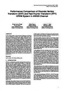
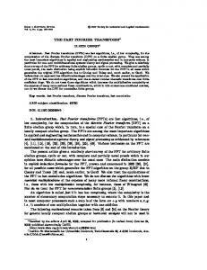
4 Implementation The FQFT algorithm was originally implemented in C++ and tested with the GNU{C++ compiler g++. C++ was chosen as programming language because of the high (and free) availability of compilers, the good performance of the executables and the elegant concepts of object oriented programming. As there are many institutes still working with Khoros 1 in image processing, an interface for using the classes in that system has been implemented, too. The main task of the implementation had been to adapt the in{ and output operations to the Khoros 1 system. The code has been tested with the Sun C++ compiler. The pictures below show a two{dimensional sinusoidal created with Khoros rad (size 512512, frequency in X direction: 0:1 rad pix , frequency in Y direction: 0:02 pix ) on the left and its magnitude{quaternionic{spectrum on the right.

sinusoidal

magnitude{quaternionic{spectrum

4.1 Classes The C++ implementation mainly consists of two classes: -

Quat domain

is the encoding of the quaternion algebra. The data is contained in double{ valued members, so the algorithms should be exact enough for most applications in image processing. Apart from the standard operations, there are some special multiplications and other operations.

Quat


24

Due to the de nition of the FQFT there are only multiplications with i{quaternions from the left and j{quaternions from the right (see (36), (41) and (45)). This fact is used to optimise the operators for multiplication: : The object (general quaternion) is multiplied with an i{quaternion. Complexity: eight multiplications and four additions.

imult()

: The object (general quaternion) is multiplied with a j{quaternion. Complexity: eight multiplications and four additions.

jmult()

: The object (itself an i{quaternion) is multiplied with an i{quaternion. Complexity: four multiplications and two additions.

imulti()

: The object (itself a j{quaternion) is multiplied with a j{quaternion. Complexity: four multiplications and two additions.

jmultj()

A division of a quaternion by a real number was implemented for normalising the domain in the inverse transform (41). This routine is named rdiv. Its complexity is four divisions. In order to get the exponential term (27) easily, a special constructor was implemented to obtain a quaternion from its polar representation. Thus, Quat('i',) returns the quaternion (cos; sin; 0; 0). The same applies for j. Besides, the three non{trivial automorphisms ; and are implemented in alpha() beta() and gamma() according to (7). The multiplications imult and jmult introduced above are combined with the automorphisms in the following way: involution of q multiplication of q with base function equivalent operation alpha

imult

aimult

alpha

jmult

ajmult

beta

imult

bimult

beta

jmult

bjmult

gamma

imult

gimult

gamma

jmult

gjmult


25

Hence, in order to apply the involution to a quaternion q and to multiply it with the i{quaternion wi afterwards, q.aimult(wi) is used. All operations also exist in the reverse order (multiplication rst, then involution), called imulta etc. The following standard operators are implemented: + according to (3) - according to (3) * according to (4) abs() magnitude according to (6) > instream operator (see below) r() real part i() i{imaginary part j() j{imaginary part k() k{imaginary part Finally, a standard{ and a copy{constructor are de ned. The outstream operator writes the quaternion as a four{tuple in the form (a, b, c, d), where a is the real part, b is the i{imaginary part, c is the j{imaginary part and d is the k{imaginary part. The instream operator reads either a real number x and returns (x, 0, 0, 0) or a four{tuple in the form mentioned above. If one or more components are omitted, zeroes are assumed as remaining components. The implementation is contained in Quat.C and Quat.h. The class domain is the encoding of a two{dimensional domain of quaternions. It represents either the spatial or the spectral domain. It is the base for the fast transform. The class has stream{operators for the PGM{raw{grey format (P5), which facilitates the reading and writing of images, and an internal format based on quaternions in form of a four-tuple in ascii{code (Q1{Format) or in binary code (Q2) in order to exchange spectra (machine dependent). The size of the domain is stored in size and the mode of writing it to a stream is represented by pgm and ascii.


26

The following operators are implemented: outstream operator (see below) >> instream operator (see below) () subscribing operator (with index{check) = assigning operator len() accessor of the member size setpgm() mutator of the member pgm setascii() mutator of the member ascii DQFT() discrete QFT according to (11) iDQFT() inverse DQFT according to (13) FQFT() fast QFT according to (36) and (37) iFQFT() inverse FQFT according to (45) and (42)