Nov 4, 2016 - This algorithm is based on a global linear interpolation .... Mf is a minimal fast linear subspace associated with a singularly perturbed vector.
arXiv:1611.01341v1 [math.NA] 4 Nov 2016
FAST-SLOW VECTOR FIELDS OF REACTION-DIFFUSION SYSTEMS V.BYKOV*, Y.CHERKINSKY**, V.GOL’DSHTEIN**, N.KRAPIVNIK**, U.MAAS*, Abstract. A geometrically invariant concept of fast-slow vector fields perturbed by transport terms (describing molecular diffusion processes) is proposed in this paper. It is an extension of our concept of singularly perturbed vector fields to reaction-diffusion systems. Fast-slow vector fields can be represented locally as "singularly perturbed systems of PDE". The paper focuses on possible ways of original models decomposition to fast and slow subsystems. We demonstrate that transport terms can be neglected (under reasonable physical assumptions) for fast subsystem. A method of analysis of slow subsystem as an evolution of singularly perturbed profiles along slow invariant manifolds was discussed in our previous work [1]. This paper is motivated by an algorithm of reaction-diffusion manifolds (REDIM) [2, 3, 4]. It can be considered as its theoretical justification extending it from a practical algorithm to a robust computational procedure under some reasonable physical assumptions. A practical application of the proposed algorithm for numerical treatment of reaction-diffusion systems is demonstrated.
1. Introduction The decomposition of complex systems into simpler subsystems using different rates of changes (multiple time scales) for different subsystems is widely used in physical and engineering models [5]-[11]. The main difficulty for complex realistic models study is the "hidden", implicit nature of the time scales of original systems of governing equations. A formal mathematical basis for such procedures is based on the notion of singularly perturbed vector fields [12]. Roughly speaking a singularly perturbed vector field (SPVF) F (z, ε) is a vector field defined in a domain G of Euclidian space Rn that depends on a small parameter ε ≥ 0 such that for any point z F (z, 0) belongs to an a priori fixed fast subspace Mf (z) of smaller dimension - dim Mf (z) < n. Moreover, the dimension of Mf (z) does not depend on the choice of the point z. Thus, the vector field F (z, ε) can be decomposed into a fast subfield that belongs to the fast subspace Mf (z) and its complement represents a slow subfield. Of course this is not a formal description, which is more sophisticated. Note, if Mf (z) does not depend on x then the vector field F (z, ε) represents (by definition) a linearly decomposed singularly perturbed vector field. Accordingly, the notion of the linearly decomposed singularly perturbed vector field is a geometrical analog of a singularly perturbed systems of ordinary differential equations. A formal concept (a theory of SPVFs) can be useful for practical applications if it is supported by an identification algorithm for fast subfields [13]. In previous papers we construct and discussed an algorithm for linearly decomposed singularly 1
2
V.BYKOV*, Y.CHERKINSKY**, V.GOL’DSHTEIN**, N.KRAPIVNIK**, U.MAAS*,
perturbed vector fields [14]. This algorithm is based on a global linear interpolation procedure for an original vector field that we call a global quasi-linearization (GQL) (see e.g. [13, 3]). The theory of singularly perturbed vector fields represents a coordinate free version of singularly perturbed systems of ordinary differential equations (ODE) [15] - [17]. It cannot be used in the original form for study the influence of transport processes of reaction-diffusion system. Thus, the main formal object of our current study is F(z, x, ε) := F (z, ε) + L(z, x, ε) and it combines a singularly perturbed vector field F (z, ε) (reaction term) and a linear operator typically of second order (diffusion term). Here x belongs to a set Vs in Euclidian space Rs , s ≤ 3. Typically it is a segment [0, L] or closed parallelogram. We suppose that fast reaction terms are much faster then corresponding transport processes, that leads to a formal assumption limε→0 L(z, x, ε) = 0, i.e. F(z, x, 0) = F (z, 0). This makes the extension of the theoretical framework straightforward. 2. General formal Notion of Fas-Slow Vector Fields In this section we adapt the main formal framework of singularly perturbed vector fields [12] to fast-slow vector fields of reaction-diffusion systems. Now, we recall a standard definition of vector bundles and use vector/fiber bundles as a formal substitute for so-called nonlinear coordinate systems. Definition. A vector bundle ξ over a connected manifold N ⊂ Rm consists of a set E ⊂ Rm (the total set), a smooth map p : E → N (the projection) which is onto, and each fiber Fxξ = p−1 (x) is a finite dimensional affine subspace. These objects are required to satisfy the following condition: for each x ∈ N , there is a neighborhood U of x in N , an integer k and a diffeomorphism ϕ : p−1 (U ) → U × Rk such that on each fiber ϕ is an isomorphism of vector spaces. Note that, all fibers have to be of the same dimension k. Definition 1. Call a domain V ⊂ Rn a structured domain (or a domain structured by a vector bundle) if there exists a vector bundle ξ and a diffeomorphism ψ : V → U onto an open subset U ⊂ E, where E is the total set of ξ.
Fix a parametric family of smooth fast-slow vector fields F (z, x, δ) := Φ(z, δ) + L(z, x, δ) defined in a domain V ⊂ Rn for any 0 < δ < δ0 . Here δ0 is a fixed positive number and δ is a small positive parameter (an explicit form of small parameter in the system is needed at least in initial stage); Φ(z, δ) is a singularly perturbed vector field, L(z, x, δ) is a linear differential operator such that limε→0 L(z, x, δ) = 0 A corresponding system of PDE’s is ∂z = F(z, x, δ) = Φ(z, δ) + L(z, x, δ). (2.1) ∂t Definition 2. Suppose that V is a domain structured by a vector bundle ξ and a diffeomorphism ψ. For any point z ∈ G call Mz := ψ −1 (p−1 (ψ(z) ∩ U ) a fast manifold associated with the point z. Call the set of all fast manifolds Mz a family of fast manifolds of V . By construction any point z ∈ G belongs to only one fast manifold. If z 6= z1 either Mz ∩ Mz1 = ∅ or Mz = Mz1 . The dimension of any manifold Mz is the same. Denote this dimension by nf and call it the fast dimension of G.
FAST-SLOW VECTOR FIELDS OF REACTION-DIFFUSION SYSTEMS
3
A family of fast manifolds Mz is linear if there exists a linear subspace Lf of Rn such that Mz = {z} + Lf for any z ⊂ V . Call Lf a fast subspace. This is a simplest possible "linear" situation. Using a corresponding linear change of variables it is possible to move Lf to a coordinate subspace like in the case of the standard SPS theory [16]. Denote by T Mz a tangent space to Mz at the point z. Definition 3. A parametric family (z, δ) : V → Rn of vector fields defined in a domain V structured by a vector bundle ξ and a diffeomorphism ψ is an asymptotic singularly perturbed vector field if limδ→0 Φ(z, δ) ∈ T Mz for any z ∈ V and the structure of the domain G is minimal for the vector field Φ(z, δ) : G → Rn in the following sense. There is no a proper vector subbundle ξ1 of the vector bundle ξ such that Φ(z, δ) : V → Rn is an asymptotic singularly perturbed vector field in a domain V structured by the vector subbundle ξ1 and the same diffeomorphism ψ. Remark. This property of minimality means that it is not possible to reduce the dimension of fast manifolds {Mz } using subbundles. From this point outwards, without loss of generality, we suppose that a family of fast manifolds {Mz } associated with a singularly perturbed vector field Φ(z, δ) is minimal. For a linear family of fast manifolds associated with a singularly perturbed vector field Φ(z, δ) the property of minimality can be written in a rather simple way. If Mf is a minimal fast linear subspace associated with a singularly perturbed vector field Φ(z, δ) then dimension nf = dim Mf cannot be reduced. Call this minimal subspace Mf a linear subspace of fast motions of Φ(z, δ). 2.1. Fast-slow decomposition of fast-slow vector fields. Fix an asymptotic fast-slow vector field F(z, x, δ). Suppose {Mz } is a fast family associated with F (z, x.δ) and the fast dimension of {Mz } is nf . Then the vector field F(z, x, δ) is a sum of two vector fields Ff (z, x, δ) := P rf Φ(z, δ) + P rf L(z, x, δ) and Fs (z, x, δ) := F(z, x, δ)−P rf F(z, s, δ). Here P rf Φ(z, δ) is a projection of Φ(z, δ) onto the tangent space T Mz of the fast manifold Mz , Lf (z, x, δ) := P rf L(z, x, δ) is the restriction of the linear differential operator L(z, x, δ) on T Mz and Ls (z, x, δ) is a similar projection of F(z, x, δ) onto the linear subspace T M z of slow motions that is orthogonal to T Mz . Call an asymptotic fast-slow vector field F(z, x, δ) a uniformly asymptotic fastslow vector field (or simply a uniform fast-slow vector field) if lim sup |P rs F(z, δ)| = 0.
δ→0 z∈V
Denote ε := supz∈V |P rs Φ(z, δ)| which is a new small parameter, ε < ε0 = supz∈V |P rs Φ(z, δ0 )|; F (z, δ) := P rf Φ(z, δ) is the fast subfield and G(z, δ) := P rs Φ(z,δ) supz∈V |P rs Φ(z,δ)| is a slow subfield of Φ(z, δ). Then the vector field F(z, δ) is a linear combination of its fast and slow subfields i.e. (2.2) where
F(z, x, δ) = Ff (z, x, δ) + εFs (z, x, δ).
4
(2.3)
V.BYKOV*, Y.CHERKINSKY**, V.GOL’DSHTEIN**, N.KRAPIVNIK**, U.MAAS*,
Ff (z, x, δ) = [F (z, δ) + Lf (z, x, δ)] , Fs (z, x, δ) = [G(z, δ) + Ls (z, x, δ)] .
Remark the small parameter ǫ is a function of the small parameter δ. If δ → 0, then ǫ → 0. For any practical implementation of the proposed construction of singularly perturbed vector fields we have to find a way to determine the fast manifolds. For the moment we know this for the linear case i.e. for the case where all fast manifolds are parallel to a fixed linear subspace Lf . In the next section we shall discuss the linear case of fast-slow vector fields in more details. A few words about slow invariant manifolds. Suppose F (z, x, δ) = [F (z, δ) + Lf (z, x, δ)] + ε [G(z, δ) + Ls (z, x, δ)] is a fas-slow vector field. The equation F (z, 0) = 0 represents a zero approximation ε = δ = 0 of a slow invariant manifold of the fast-slow vector field F(z, x, δ). Situations with higher order approximations is more complicated. 3. Fat-slow Vector Fields with Linear Fast Subspace For any realistic complex model the small parameter δ is unknown and this fact restricts possible applications of the proposed asymptotic theory. In this section we will try explain how to adapt the asymptotic theory developed for practical problem in the simplest possible case of linear fast manifolds. Thus any fast manifold at any point z is parallel to a linear subspace Mf (z) with fixed dimension nf . Note that for many applications an assumption that Mf does not depend on z is natural. 3.1. Fast-slow decomposition. Fix a uniformly asymptotic fast-slow vector field F(z, δ). Suppose that the fast subspace Mf does not depend on z and dim Mf = nf . The vector field F(z, x, δ) is a sum of two vector fields Ff (z, x, δ) := P rf F(z, x, δ) and Fs (z, x, δ) := F(z, x, δ) − P rf F(z, δ). The uniformity condition permits us to represent a uniformly singularly perturbed vector field and a corresponding dynamical system (2.1) as a standard singularly perturbed system (SPS). A corresponding construction is now possible. Suppose u := P rf z and v := P rs z are fast and slow variables that represent a new coordinate system with nf fast variables u and ns = n − nf slow variables v; ε := supz∈V |P rs Φ(z, δ)| is a small parameter, ε < ε0 = supz∈V |P rs Φ(z, δ0 )|; F (x, y, δ) is a representation of F (z, δ) := P rf Φ(z, δ) in the new coordinate system (x, y) and G(x, y, δ) is a representation of G(z, δ) := sup P rs|PΦ(z,δ) rs Φ(z,δ)| in the new z∈V coordinate system (x, y). Hence the system (2.1) has the standard SPS form (3.1)
∂u = F (u, v, δ) + Lf (u, v, x, δ) ∂τ
∂v = εG(u, v, δ) + εLs (u, v, x, δ). dτ in the new coordinate system (u, v). (3.2)
FAST-SLOW VECTOR FIELDS OF REACTION-DIFFUSION SYSTEMS
5
Remember once again that the small parameter ǫ is a function of the small parameter δ [12]. If δ → 0, then ǫ → 0. By rescaling the time t = τε from slow to fast one we can rewrite the previous fast-slow system in an another standart form ∂u (3.3) ε = F (u, v, δ) + Lf (u, v, x, δ) ∂t ∂v = G(u, v, δ) + Ls (u, v, x, δ). dτ Under a formal substitution ε = 0 we can write an analog of slow invariant manifold (3.4)
(3.5)
F (u, v, 0) = 0.
For typical reaction-kinetic and combustion system the situation can be essentially simplified and the regular theory of singularly perturbed system of ODE can be adapted. Some additional assumptions: (1) The fast linear operator Lf (u, v, x, δ) does not depends on slow variables and the small parameter δ, i.e. to the leading order it can be written as Lf (u, x); (2) The slow linear operator Ls (u, v, x, δ) does not depends on fast variables and the small parameter δ, i.e. it can be written as L(v, x); (3) Transport processes for the fast and slow variables have the same order, because diffusion and convection processes do not depend directly on reaction processes. It means that the fast operator Lf (u, x) can be rewritten as Lf (u, x) := εL(u, x). Under these assumptions the system ( 3.33.4) can be further simplified ∂u (3.6) ε = F (u, v, δ) + εL(u, x) ∂t ∂v = G(u, v, δ) + L(v, x). dτ Call this system as a reaction-diffusion fast-slow vector field. Under a formal substitution ε = 0 we can write the same zero approximation of the slow invariant manifold:
(3.7)
(3.8)
F (u, v, 0) = 0.
3.2. Singularly perturbed vector fields: non asymptotical definition. In many practical situations the previous definition of an asymptotical fast-slow vector field F(z, x, δ) cannot be useful because a small parameter δ is unknown. Meanwhile the main geometrical idea is still useful if some previous knowledge about a scaling is known. It means that some "small" number ε0 is fixed for corresponding processes (models) and any parameter ε < ε0 can be considered as a small parameter. Suppose a smooth fast-slow vector field F(z, x) is defined in a structured domain V ⊂ Rn , z ∈ V , a parametric domain Vs , x ∈ Vs and Lf is the fast subspace. Moreover supz∈V |P rs F(z, x)| < ε0 . Suppose as well, as in the previous subsection that u := P rf z and v := P rs z are fast and slow variables that represent a new coordinate system with nf fast variables u and ns = n − nf slow variables v; ε := supz∈V |P rs F(z)| is a small
6
V.BYKOV*, Y.CHERKINSKY**, V.GOL’DSHTEIN**, N.KRAPIVNIK**, U.MAAS*,
system parameter; F (u, v)+Lf (u, v, x) is a representation of P rf F(z) and G(u, v)+ P rs Φ(z) Ls (u, v, x) is a representation of supz∈V |P rs Φ(z)| in the new coordinate system (u, v). Hence the system (2.1) has the following form: (3.9)
∂u = F (u, v) + Lf (u, v, x) ∂τ
(3.10)
∂v = ε [G(u, v) + Ls (u, v, x)] . dτ
in the new coordinate system (u, v) and F(u, v, ε) := F (u, v) + Lf (u, v, x) + ε [G(u, v) + Ls (u, v, x)] is a fast-slowvector field. Similar modifications can be used for cases (3.3)-(3.4) and (3.6)-(3.7). 4. Fast motion time estimates In this section we justify a formal definitionof slow manifold estmatimg influence of transport for the system (3.6)-(3.7) that represents a a reaction-diffusion fast-slow vector field. 4.1. Fast motion time estimates for ODE. Consider first the system of ordinary differential equations in the standard SPS form
(4.1)
dx dt = f (x, y), ε dy dt = g(x, y).
where x ∈ Rn , y ∈ Rm .Here x is a slow vector, y is a fast vector. Suppose that (x0 , y0) is an initial data for this system and g(x0 , y0 ) 6= 0 . The subspace Lx0 = [(x, y) ∈ Rn+m : x = x0 ] is a fast subspace that contains (x0 , y0 ). Our main assumption here is simplicity of the slow invariant manifold g(x, y) = 0. It means that tye equation g(x, y) = 0 a zero approximation ε = 0 of a stable invariant slow manifold. It means that any fast subspace has a one point intersection (x0 , ys ) with the slow invariant manifold that is an attractive singukar point of the fast subsytem ε dy dt = g(x, y). Our next assumption used is a simplicity of fast dynamics. We suppose that a length of the fast trajectory, that joints points (x0 , y0 ) and the fast singular point (x0 , ys ) is less than 2|y0 − ys |. √ For any ε > 0 the open set F√ε := {(x, y) ∈ Rn+m |g(x, y)| < ε. Outside of the slow neiboobhood F√ε of the slow manifold Fs := {(x, y)|g(x, y) = 0} the fast componenet of the vector field Φ(x, y) := {f (x, y), 1ε g(x, y) satisffies to the inequality 1ε |g(x, y) ≥ √1ε . The fast trajectory with the initial point y0 is a curve ϕ : [0, ∞) → Lx0 where 0 ≤ t < ∞ and ϕ′ (t) = 1ε g(x0 , ϕ(t)). Under our assumptions its length Z ∞ Z ∞ 1 ′ |g(x0 , ϕ(t))|dt ≤ 2|y0 − ys |. lϕ := |ϕ (t)|dt = ε 0 0
FAST-SLOW VECTOR FIELDS OF REACTION-DIFFUSION SYSTEMS
7
√ ε2|y0 − ys | we have Z t0 Z t0 1 1 √ dt = 2|y0 − ys |. |g(x0 , ϕ(t))|dt ≥ lϕ = ε ε 0 0 √ It means that for any t0 > 2ε|y0 − ys | the point ϕ(t0 ) belongs √ to the slow √ neiboobhood F ε . Therefore the fast motion time is less than 2ε2y0 − ys |. After this time the solution of the fast subsystem ε dy dt = g(x, y) belongs to the slow neiboorhood F√ε . The influence of the slow subsytem to this estimate is negligable. For any t0 >
4.2. Fast motion time estimates for models with diffusion. Consider the system of PDEs
(4.2)
du(x,t) = f (u(x, t), v(x, t)) + L1,x (u(x, t), v(x, t)) dt dv(x,t) 1 = dt ǫ g (u(x, t), v(x, t)) + L2,x (u(x, t), v(x, t))
Here 0 ≤ x ≤ 1 and L1,x , L2,x are elliptic differential operators of the second order. We treat the transport term as slow comparatively with the fast component of the vector field, i.e |L1,x (u(x, t), v(x, t))| ≤ K|g (u(x, t), v(x, t)) | |L2,x (u(x, t), v(x, t))| ≤ K|g (u(x, t), v(x, t)) | outside of the slow neiboobhood F√ε . Here K is a constant that typically do not exceed 3. An additional assumption for the fast subsytem is |L2,x (u(x, 0), v(x, t))| ≤ K|g (u(x, ), v(x, t)) | for any x ∈ [0, 1] and any t ∈ [0, ∞). The slow system evolution is then controlled by u(x, t) = (u1 (x, t), ..., ums (x, t)) , which are assumed to change slowly comparatively to the fast variables � v(x, t) = v1 (x, t), ..., vmf (x, t) , ms + mf = n.
The transport diffusion terms are represented first by very general and smooth differential operators L1,x (u(x, t), v(x, t)), L2,x (u(x, t), v(x, t)) Initial data for the system are (4.3)
u(x, 0) = u0 (x), v(x, 0) = v0 (x).
Our main goal is to check influence of the transport operators to the fast time estimates obtained in the previous section. Fix x0 ∈ [0, 1] and check length of the fast trajectory that belongs to the fast subspace Lu(x0 ,0) , its starting point is y0 := v(x0 , 0) and its final point is ys := Lu(x0 ,0) ∩ Fs .
8
V.BYKOV*, Y.CHERKINSKY**, V.GOL’DSHTEIN**, N.KRAPIVNIK**, U.MAAS*,
The fast trajectory with the initial point y0 is a curve ϕ : [0, ∞) → Lu(x0 ,0) where 0 ≤ t < ∞ and ϕ′ (t) = 1ε g(x0 , ϕ(t) + L2,x (u(x, t), v(x, t))). Under our assumptions its length Z ∞ Z ∞ 1 ′ lϕ := |ϕ (t)|dt = ε g(u(x0 , 0), ϕ(t)) + L2,x (u(x0 , 0), v(x0 , t))) dt ≤ 0 0 Z ∞ Z ∞ 1 g(u(x0 , 0), ϕ(t)) dt + |L2,x (u(x0 , 0), v(x0 , t)))| dt ≤ 2|y0 − ys | ε 0 0 Z ∞ 2|y0 −ys |+ K |g(u(x0 , 0), ϕ(t))| dt ≤ 2|y0 −ys |+εK2|y0 −ys | = 2(1+εK)|y0 −ys |. 0 √ It means that for any t0 > 2ε(1+εK)|y0 −ys | the point ϕ(t0√) belongs to the slow neiboobhood F√ε . Therefore the fast motion time is less than 2ε(1 + εK)|y0 − ys |. 1 After this time the solution of the fast subsystem dy dt = ǫ g (u(x0 , 0), v(x0 , t)) + L2,x (u(x0 , 0), v(x0 , t)) belongs to the slow neiboorhood F√ε . The influence of the slow subsytem to this estimate is negligable. 5. Singularly perturbed profiles and the REDIM approach In this section the REDIM method will be discussed as a method to construct the manifold approximating the evolution of the detailed system solution profiles. Recall definition of singularly perturbed profiles [1]. Accordingly, we are looking for the following representation of the system 2.1:
(5.1)
(
du(x,t) = Fs (u(x, t), v(x, t)) + L1,x (u(x, t), v(x, t)) dt dv(x,t) = 1ǫ Ff (u(x, t), v(x, t)) + L2,x (u(x, t), v(x, t)) dt
The slow system evolution is then controlled by u(x, t) = (u1 (x, t), ..., ums (x, t)) , which are assumed to change slowly comparatively to the fast variables � v(x, t) = v1 (x, t), ..., vmf (x, t) , ms + mf = n. Initial data for the system 5.1 are
(5.2)
u(x, 0) = u0 (x), v(x, 0) = v0 (x)..
∼ O (1) while that functions Fs , Ff are of the same order. Then dU dt dVRecall � ∼ O 1 . We suppose also that operators L1,x (u(x, t), v(x, t)), L2,x (u(x, t), v(x, t)) dt ε has the same order as Fs , Ff . Recall that the zero approximation S of the slow invariant manifold in the phase space (u, v) (the space of species) is represented in the implicit form Ff (u, v) = 0 The initial profile is Γ0 (x) := (u0 (x), v0 (x)); u0 (x) = u(x, 0), v0 (x) = v(x, 0). Denote Γ (x, t) a profile that is the solution of (5.1) at time t with the initial profile (initial data) Γ0 (x). Note that the singularly perturbed structure of the system (5.1) was investigated in [1], but for a system in the general form 2.1 this information is absent, thus, the question how to find (5.3)
Ff (u(x, t), v(x, t)) = 0,
FAST-SLOW VECTOR FIELDS OF REACTION-DIFFUSION SYSTEMS
9
as e.g. the zero order approximation Γ0 (x, t) of Γ (x, t) which belongs to S for all t, represents the main problem of model reduction for a reaction-diffusion system (of a PDEs system). The set RM := ∪t∈(0,∞) Γ (x, t) is called the reaction-diffusion manifold (REDIM) and RM0 := ∪t∈(0,∞) Γ0 (x, t) is its zero approximation (for ǫ = 0). Note that if the dimension of the profile is equal to s (dim Γ (x, t) = s), then dim RM = dim RM0 = s + 1. 5.1. REDIM. In the framework of the REDIM [2], the manifold of the relatively slow profile evolution S is constructed/approximated by using the so-called Invariance Condition (see e.g. [18, 19, 2] for more details). The construction of an explicit representation of a low-dimensional manifold S = {z : z = z(θ), θ ∈ Rms },
(5.4)
starts from an initial solution z = z0 (θ) and then it is integrated with the vector field of the PDEs reaction-diffusion system: (5.5)
∂z(θ) = (I − zθ zθ+ )(Φ(z(θ), δ) + L(z(θ), x, δ)), ∂τ
where the evolution of the manifold along its tangential space is forbidden by restricting it to the normal (or transverse) subspace. It is given by the local projector: P rT M ⊥ = (I − zθ zθ+ ), here I identity matrix, zθ denotes the tangential subspace and zθ+ is the Moore-Penrouse pseudo-inverse of the local coordinates Jacobi matrix zθ . Now, if the assumption of the study is valid, the manifold will evolve within fast manifolds of the vector field and will converge asymptotically to an invariant system manifold S approximating the slow profile evolution. ψb 1.0
Z 0.5
ψeq 2.0 1.5
0.0 1.0
1.0
Y
0.5
X
0.5 0.0
Figure 5.1. System state space (X,Y,Z) is shown. 2D slow manifold for the pure homogeneous system (6.3) is represented by a mesh. System stationary solution profile (6.6), black solid curve) in 1D case corresponds to 1D REDIM due to dimensional considerations. The approximation of the fast part of the homogeneous system (6.3) solution trajectory is shown by the dashed line.
10
V.BYKOV*, Y.CHERKINSKY**, V.GOL’DSHTEIN**, N.KRAPIVNIK**, U.MAAS*,
6. Analysis of 3D Michaelis-Menten model with the Laplacian Operator The 3D Michaelis-Menten model is considered here as illustrative example of the REDIM approach. The original mathematical model of the enzyme biochemical system consists of three ODEs (6.1) (6.2) (6.3)
dX = −XZ + L1 (1 − Z − µ(1 − Y )) dt L4 dY (1 − Y ) = −L3 Y Z + dt L2 dZ L4 1 ((−XZ + 1 − Z − µ(1 − Y )) + µ) − L3 Y Z + (1 − Y ))) = dt L2 L2
The system parameters are taken as L1 = 0.99, L2 = 1, L3 = 0.05, L4 = 0.1, µ = 1 (see e.g. [1, 11] for details and references). By taking the 1D diffusion into account we obtain the following PDEs system with the constant diffusion coefficient δ = 0.01: ∂X = −XZ + L1 (1 − Z − µ(1 − Y )) + δ∆X ∂t L4 ∂Y (6.5) (1 − Y ) + δ∆Y = −L3 Y Z + ∂t L2 ∂Z L4 1 (6.6) ((−XZ + 1 − Z − µ(1 − Y )) + µ) − L3 Y Z + (1 − Y ))) + δ∆Z = ∂t L2 L2
(6.4)
The system (6.6) is considered with the following initial and boundary conditions:
(6.7)
(6.8)
(6.9)
X(t, 0) = Xeq Y (t, 0) = Yeq Z(t, 0) = Zeq X(t, 1) = 2 Y (t, 1) = 0 Z(t, 1) = 1 X(0, x) = (2 − Xeq )x + Xeq Y (0, x) = (−Yeq )x + Yeq Z(0, x) = (1 − Zeq )x + Zeq
Here (Xeq , Yeq , Zeq ) are coordinates of the equilibrium point and x is spatial variable. Initial conditions are chosen to be a straight lines, they satisfy the general assumption - join initial and equilibrium values on the boundaries. First, several numerical experiments were performed. A 2D slow manifold for homogeneous system (6.3) was found. Stationary system (6.6) solution profile was also integrated. Figure 5.1 shows a connection between the zero approximation of the slow manifold and the profile of the stationary system solution of the PDE in the original coordinates (X, Y, Z). In Fig. 5.1 the system solution profile can be roughly subdivided into two parts: the slow part of the stationary solution that is very close to the slow manifold of the homogeneous system and second one, which is influenced by the diffusion term.
FAST-SLOW VECTOR FIELDS OF REACTION-DIFFUSION SYSTEMS
11
1.0
Z
0.5
0.0 1.0
2.0 1.5
0.5
1.0
Y
0.5
X
0.0
Figure 6.1. REDIM manifold (dashed line), exact stationary solution of the original PDE system (think line). As in the previous section the main assumption remains the transport term is slow compared with the fast vector field. By applying the REDIM approach the stationary solution of the following system should represent the one-dimensional REDIM. ∂Ψ (6.10) = (I − Ψθ Ψ+ θ )(FR + FD ) ∂t (6.11) where following notations have been used, I 1 0 I = 0 1 0 0
state space vector:
itentity matrix: 0 0 , 1
X Ψ = Y , Z
projection matrix to the manifold tangent space 2 Xθ Xθ Yθ 1 Yθ Xθ Yθ2 Ψθ Ψ+ θ = Xθ2 + Yθ2 + Zθ2 Zθ Xθ Zθ Yθ and vector fields of reaction and diffusion terms Xθθ FD = δθx2 Yθθ , Zθθ
Xθ Z θ Yθ Zθ , Zθ2
12
V.BYKOV*, Y.CHERKINSKY**, V.GOL’DSHTEIN**, N.KRAPIVNIK**, U.MAAS*,
−XZ + L1 (1 − Z − µ(1 − Y )) 4 −L3 Y Z + L FR = L2 (1 − Y ) 1 L2 ((−XZ + 1 − Z − µ(1 − Y )) + µ) − L3 Y Z +
L4 L2 (1
− Y )))
.
Here θ is the manifold parameter and θx is the gradient of the manifold parameter in FD . Now by using θ = X as a local manifold parameter, the system (6.10) can be simplified to only two equations for Y = Y (θ) and for Z = Z(θ). They were integrated and the stationary solution has been found for 1D REDIM, which is completely coincides with the system stationary profile (see Fig. 6.1). Figure 6.2 shows a connection between the 2D REDIM, initial solution for the REDIM and/or slow homogeneous system manifold as in Figs. 5.1 and 6.1. The stationary solution profile of the system illustrates the implementation and quality of the the REDIM approach to approximate the low- dimensional invariant manifold of relatively slow evolution of the reacting-diffusion system.
Figure 6.2. On the left: 2D slow homogeneous system manifold, in the middle: an initial solution for the REDIM and 2D REDIM manifold (shown on the right), exact stationary solution of the original PDE system (shown by thick line).
7. Conclusions The framework for manifolds based model reduction of the reaction-diffusion system has been established in the current work. This follows the original ideas of the singularly perturbed vector fields developed earlier. Within the suggested concept the problem of model reduction is treated as restriction of the original system to a low-dimensional manifold. The manifold encounters the stationary states of the degenerate fast subfield of the vector field defined by the reactiondiffusion system. The main assumption of weak dependence of the fast system subfiled of the PDE vector field has been formulated. Under this assumption the theory of singularly perturbed vector fields was extended to the the systems with the molecular transport included. The developed framework can be used to justify the so-called REDIM method developed for reacting flow systems. For illustration MichaelisMenten chemical kinetics model is extended to describe reaction-diffusion process. This example is used in the application to illustrate the method and the suggested framework.
FAST-SLOW VECTOR FIELDS OF REACTION-DIFFUSION SYSTEMS
13
Acknowledgments Financial support by the DFG within the German-Israeli Foundation under Grant GIF (No: 1162-148.6/2011) is gratefully acknowledged. References [1] Bykov V., Cherkinsky, Y., Mordeev, N., Gol’dshtein, V., Maas, U., Singularly Perturbed Profiles, submitted, 2016; Preprint: https://arxiv.org/pdf/1607.00486.pdf [2] Bykov, V., Maas, U., 2007, The Extension of the ILDM Concept to Reaction-Diffusion Manifolds, Combustion Theory and Modelling (CTM), 11 (6), 839-862. [3] Bykov, V., Maas, U., 2009, Problem Adapted Reduced Models Based on Reaction-Diffusion Manifolds (ReDiMs), Proc. Comb. Inst., 32(1): 561-568. [4] Maas, U., Bykov, V., 2011, The Extension of the Reaction/Diffusion Manifold Concept to Systems with Detailed Transport Models, Proc. Comb. Inst., 33(1):1253-1259. [5] U. Maas, S.B. Pope, Simplifying Chemical Kinetics: Intrinsic Low-Dimensional Manifolds in Composition Space, Combustion and Flame, 117, 99-116 (1992). [6] S.H. Lam, D.M. Goussis, The GSP method for simplifying kinetics, International Journal of Chemical Kinetics, 26, 461-486 (1994). [7] C. Rhodes, M. Morari, S. Wiggins, Identification of the Low Order Manifolds:Validating the Algorithm of Maas and Pope, Chaos, 9, 108-123 (1999). [8] H. G. Kaper, T.J. Kaper, Asymptotic Analysis of Two Reduction Methods for Systems of Chemical Reactions, Argonne National Lab, preprint ANL/MCS-P912-1001 (2001). [9] I.Goldfarb, V.Gol’dshtein, U.Maas, Comparative Analysis of Two Assymptotic Approaches Based on Integral Manifolds, IMA J. of Applied Mathematics, 69, 353-374 (2004). [10] Marc R. Roussel and Simon J. Fraser, Global analysis of enzyme inhibition kinetics. J. Phys. Chem. 97, 8316-8327; errata, ibid. 98, 5174, (1993). [11] Marc R. Roussel and Simon J. Fraser, Invariant manifold methods for metabolic model reduction. Chaos 11, 196-206 (2001). [12] Bykov, V., Goldfarb, I., Gol’dshtein, V., 2006, Singularly Perturbed Vector Fields, Journal of Physics: Conference Series, 55, 28-44. [13] Bykov, V., Gol’dshtein, V., Maas, U., 2008, Simple Global Reduction Technique Based on Decomposition Approach, Combustion Theory and Modelling (CTM), 12 (2), 389-405. [14] Bykov, V., Maas, U., 2009, Investigation of the Hierarchical Structure of Kinetic Models in Ignition Problems, Z. Phys. Chem., 223 (4-5), 461-479. [15] V. Gol’dshtein, V. Sobolev, Integral manifolds in chemical kinetics and combustion, In Singularity theory and some problems of functional analysis, American Mathematical Society, 73-92 (1992). [16] N. Fenichel, Geometric singular perturbation theory for ordinary differential equations, J Differential Equations, 31, 53-98 (1979). [17] Yu.A.Mitropolskiy, O.B.Lykova, Lectures on the methods of integral manifolds (Kiev: Institute of Mathematics Ukrainen Akademy of Science, in Russian) (1968). [18] A.Gorban, I.Karlin, Methods of invarinat manifoldsfor kinetic problems, Journal of Chemical kinetics, 396, 197-403 (2002). [19] A.Gorban, I.Karlin, A.Zinoviev, Constructive methods of invariant manifolds for kinetic problems, Physics Reports, 396, 197-403 (2004). *Institute for Technical Thermodynamics, Karlsruhe University, Karlsruhe, Germany **Department of Mathematics, Ben-Gurion University, Beer Sheva, Israel