Fast Solution of Periodic Optimal Control Problems in Automobile Test

Proceedings of the 47th IEEE Conference on Decision and Control Cancun, Mexico, Dec. 9-11, 2008

TuC10.5

Fast solution of periodic optimal control problems in automobile test-driving with gear shifts Sebastian Sager, Christian Kirches, Hans Georg Bock Interdisciplinary Center for Scientific Computing (IWR) Ruprecht-Karls-Universit¨at Heidelberg D-69120 Heidelberg, Germany {sebastian.sager | bock | christian.kirches}@iwr.uni-heidelberg.de

Abstract— Optimal control problems involving timedependent decisions from a finite set have gained much interest lately, as they occur in practical applications with a high potential for optimization. A typical application is automobile driving with gear shifts. Recent work [7], [8], [9] lead to a tremendous speedup in computational times to obtain optimal solutions, allowing for more complex scenarios. In this paper we extend a benchmark mixed-integer optimal control problem to a more complicated case in which a periodic solution on a closed track is considered. Our generic solution approach is based on a convexification and relaxation of the integer control constraint. It may also be used for other objectives, such as energy minimization. Using the direct multiple shooting method we solve the new benchmark problem and present numerical results.

I. I NTRODUCTION Mixed–integer optimal control problems (MIOCPs) in ordinary differential equations (ODEs) have gained increasing interest over the last years, see [12], [13], [14] for further references. This is probably due to the fact that the underlying processes have a high potential for optimization. Typical examples are the choice of gears in transport, [7], [8], [14], [9], or processes in chemical engineering involving on-off valves, [13]. From a mathematical point of view the integer requirement makes this problem class extremely challenging. The fact that optimal trajectories for problems in which the integrality constraint has been relaxed may contain sensitivity-seeking or path-constrained arcs that have no meaning from the application point of view requires thus efficient and stable algorithms. Although the first MIOCPs, namely the optimization of subway trains that are equipped with discrete acceleration stages, were already solved in the early eighties for the city of New York, [4], the so–called indirect methods used there do not seem appropriate for generic large–scale optimal control problems with underlying nonlinear differential algebraic equation systems. Instead direct methods have become the methods of choice for most practical problems. See [2] for an overview. In direct methods infinite–dimensional control functions are discretized by basis functions and corresponding finite– dimensional parameters that enter into the optimization problem. The drawback of direct methods with binary control functions obviously is that they lead to high–dimensional

978-1-4244-3124-3/08/$25.00 ©2008 IEEE

vectors of binary variables. For many practical applications a fine control discretization is required, however. Therefore, techniques from mixed–integer nonlinear programming like Branch&Bound or Outer Approximation will work only on limited and small time horizons because of the exponentially growing complexity of the problem, [15], [9]. We propose to use an outer convexification with respect to the binary controls. The reformulated control problem has two main advantages compared to standard relaxations1 . First, especially for time-optimal control problems, the optimal solution of the relaxed problem often exhibits a bang– bang structure, and is thus already integer feasible. Second, theoretical results have recently been found, [12], [14], that show that even for path-constrained and sensitivity-seeking arcs the optimal solution of the relaxed problem yields the exact lower bound on the minimum of the integer problem. This allows to calculate the loss of performance, if a coarser control discretization grid, a simplified switching structure for the optimization of switching times, or heuristics are used. In a recent publication [9], the strength of this approach was shown by solving a benchmark mixed-integer control problem which has its origin in automobile testdriving and involves discrete controls for the choice of gears. Time-optimal reference solutions obtained by a direct approach, solving a mixed-integer nonlinear program via Branch&Bound were known for this problem, [7]. The new approach reproduces the published reference solutions with computational costs reduced by several orders of magnitude. This gain in computational efficiency allows to extend the problem to more complicated scenarios. In this paper we investigate optimal long-term solutions on closed tracks, incorporated by periodicity constraints of the type x(0) = x(T ) into the optimization problem. The numerical results show the broad applicability and merit of the proposed algorithm. II. P ROBLEM F ORMULATION In this section we will give a description of the car model and the reference test course. 1 in the following we will use the expression relaxed whenever a control constraint µ(t) ∈ {a1 , . . . , an } is relaxed to w(t) ∈ [a1 , an ].

1563

47th IEEE CDC, Cancun, Mexico, Dec. 9-11, 2008

TuC10.5

A. Car model We consider a car model derived under the simplifying assumption that rolling and pitching of the car body can be neglected. Only a single front and rear wheel is modelled, located in the virtual center of the original two wheels. Motion of the car body is considered on the horizontal plane only. Four controls represent the driver’s choice on steering and velocity, and are listed in Table I. We denote the control space by U. Control wδ FB φ µ

Range [−0.5, 0.5] [0, 1.5 · 104 ] [0, 1] {1, . . . , 5}

Unit rad s

N – –

The slip angle’s denotes the deviation of the car’s direction of movement from its longitudinal axis.Its change is controlled by the steering wheel and counteracted by the sum of forces attacking perpendicular to the car’s direction of driving, 1  ˙ (5) β(t) = wz (t) − m v(t)
(Flr − FAx ) sin β(t) + Flf sin δ(t) + β(t)
 + (Fsr − FAy ) cos β(t) + Fsf cos δ(t) + β(t) .

The yaw angle representing the orientation of the car’s longitudinal axis against the horizontal coordinate axis is obtained by integrating over its change wz ,

Description Steering wheel angular veloc. Total braking force Accelerator pedal position Selected gear

˙ ψ(t) = wz (t),

which in turn is the integral over the sum of forces attacking the front wheel in direction perpendicular to the car’s longitudinal axis of orientation,

TABLE I C ONTROLS USED IN THE CAR MODEL .

w˙ z (t) =

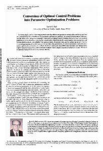
The dynamics are described by a system of ordinary differential equations. The individual system states are listed in Table II, while Figure 1 visualizes the choice of coordinates, angles, and forces. State cx cy v δ β ψ wz

Unit m m m s

rad rad rad rad s

(6)

1 Fsf lf cos δ(t) − Fsr lr Izz
− FAy eSP + Flf lf sin δ(t) .

(7)

Description Horizontal position of the car Vertical position of the car Magnitude of directional velocity of the car Steering wheel angle Side slip angle Yaw angle Yaw angle velocity Fig. 1.

TABLE II

Coordinates and forces in the single-track car model.

C OORDINATES AND STATES USED IN THE CAR MODEL .

The center of gravity is denoted by (cx , cy ) and is obtained by integrating the directional velocity,
c˙x (t) = v(t) cos ψ(t) − β(t) ,
c˙y (t) = v(t) sin ψ(t) − β(t) .

(1) (2)

Acceleration into the direction of driving is obtained from the sum of forces attacking the car’s mass m,
1 µ (Flr − FAx ) cos β(t) + Flf cos δ(t) + β(t) m (3)
 − (Fsr − FAy ) sin β(t) − Fsf sin δ(t) + β(t) .

v(t) ˙ =

The steering wheel’s angle, i.e., the angle of the front wheel w.r.t. the general orientation of the car’s longitudinal axis, is obtained from the corresponding controlled angular velocity, ˙ = wδ . δ(t)

We now list and explain the individual forces used in this ODE system. We first discuss lateral and longitudinal forces attacking at the front and rear wheels. In view of the convex reformulation we’ll undertake later, we consider the gear µ to be fixed and denote dependencies on the selected gear by µ a superscript µ like, e.g., in wmot . The side (lateral) forces on the front and rear wheels as functions of the slip angles αf and αr according to the socalled ”magic formula“ due to [11] are  Fsf,sr (αf,r ) := Df,r sin Cf,r arctan Bf,r αf,r (8)
 − Ef,r (Bf,r αf,r − arctan(Bf,r αf,r )) . The front slip angle itself is obtained from αf := δ(t) − arctan

˙ − v(t) sin β(t) lf ψ(t) v(t) cos β(t)

!

(9)

while the rear slip angle is

(4)

1564

αr := arctan

˙ + v(t) sin β(t) lr ψ(t) v(t) cos β(t)

!

.

(10)

47th IEEE CDC, Cancun, Mexico, Dec. 9-11, 2008

TuC10.5

The longitudinal force at the front wheel is composed from braking force FBf and resistance due to rolling friction FRf Flf := −FBf − FRf .

(11)

Assuming a rear wheel drive, the longitudinal force at the rear wheel is given by the transmitted engine torque Mwheel and reduced by braking force FBr and rolling friction FRr . µ The effective engine torque Mmot is transmitted twice. We µ denote by ig the gearbox transmission ratio corresponding to the selected gear µ, and by it the axle drive’s fixed transmission ratio. R is the rear wheel radius. Flrµ :=

iµg it µ Mmot (φ) − FBr − FRr . R

(12)

The engine’s torque, depending on the acceleration pedal’s position φ, is modeled as follows: µ µ µ Mmot (φ) := f1 (φ) f2 (wmot ) + (1 − f1 (φ)) f3 (wmot ),

(13) f1 (φ) := 1 − exp(−3 φ),

B. Test course We realize test courses by constraining the car’s position onto a prescribed track at any time t ∈ [t0 , tf ]. To facilitate the formulation of the extended periodic benchmark problems we chose an elliptic track with axes of a = 170 meters and b = 80 meters respectively, centered in the origin. The track’s width is W = 7.5 meters, five times the car’s width B = 1.5 meters. The set of feasible positions is hence n  X (t) = (a + r) cos η, (b + r) sin η o (22) r ∈ [−W/2, W/2] ⊂ R , η(t) = arctan

f2 (wmot ) := −37.8 + 1.54 wmot − 0.0019 f3 (wmot ) := −34.9 − 0.04775 wmot .

(15) (16)

MAX 800 =: nMIN eng ≤ neng ≤ neng := 8000,

µ wmot :=

iµg it v(t). R

(17)

The total braking force FB is controlled by the driver. For its distribution to front and rear wheels we choose FBf :=

2 FB , 3

FBr :=

1 FB . 3

(18)

The braking forces FRf and FRr due to rolling resistance are obtained from FRf (v) := fR (v)

m lf g m lr g , FRr (v) := fR (v) , (19) lf + l r lf + lr

πnMIN πnMAX eng R eng R µ ≤ v(t) ≤ 30it ig 30it iµg

C. Optimal control problem We denote with x the state vector of the ODE system and by f the corresponding right-hand side function. The vector u shall be the vector of continuous controls, whereas the integer control µ(·) will be written in a separate vector, i⊺ h i⊺ h x := cx , cy , v, δ, β, ψ, wz , u := wδ , FB , φ . With this notation, the resulting mixed-integer optimal control problem reads as min s.t. r



+ 5.038848 · 10−10 v 4 .

FAx :=

1 cw ρ A v 2 (t), 2

FAy := 0.

(21)

The model parameters m, g, lf , lr , lr , eSP , R, Izz , cw , ρ, A, it , and iµg and the Pacejka coefficients Bf,r , Cf,r , Df,r , Ef,r can be found in [7], [8], and [9].

tf

tf ,x(·),u(·),µ(·)

(20)

Finally, drag force due to air resistance is given by FAx , while we assume that no sideward drag forces (e.g., side wind) are present.

(25)

for all t ∈ T and the active gear µ(t). We write this as reng (v(t), µ(t)) ≥ 0.

where the velocity-dependent amount of friction is modeled by fR (v) := 9 · 10−3 + 7.2 · 10−5 v

(24)

in the form of equivalent velocity constraints

µ wmot

Here, is the engines rotary frequency in Hertz. For a given gear µ it is easily computed from the car’s speed by

(23)

Note that the special case cx (t) = 0 leading to η(t) = ± π2 requires separate handling. This model has a shortcome, as switching to a low gear is possible also at high velocities, although this would lead to an unphysically high engine speed. Therefore we extend it by additional constraints on the car’s engine speed

(14) 2 wmot ,

cy (t) . cx (t)

eng


x(t) ˙ = f t, x(t), u(t), µ(t) ,   cx , cy (t) ∈ X (t)

(v(t), µ(t)) ≥ 0,  wδ , FB , φ, µ (t) ∈ U,

x(t0 ) = x(tf ), cy (t0 ) = 0.

(26a) (26b) (26c) (26d) (26e) (26f) (26g)

where (Eq. 26b) through (Eq. 26e) shall hold for all t ∈ [t0 , tf ]. By employing the objective function (Eq. 26a) we strive to minimize the total time tf required to traverse the test course. As is formulated in (Eq. 26c), the car must be positioned within the test course’s boundaries X (t) at any time. The system’s periodicity constraints are given by (Eq. 26f) (plus an offset of 2π for the yaw angle ψ). The car’s initial vertical position on the track is fixed to zero without loss of generality for better comparability of results.

1565

47th IEEE CDC, Cancun, Mexico, Dec. 9-11, 2008

TuC10.5

III. G ENERAL PROBLEM CLASS AND ALGORITHM In this section we will abstract the control problem to a more general class and propose algorithms for the solution. A. General problem class The mixed-integer optimal control problem formulated in Section II-C belongs to a broader class of equality- and inequality-constrained optimal control problems on dynamic processes modeled by ODE systems. We consider the following class of optimal control problems: M tf , x(tf ), p

min tf ,p

x(·),u(·),µ(·)

s.t.




x(t) ˙ = f t, x(t), u(t), µ(t), p
0 ≤ c t, x(t), u(t), p 0≤

0=

(27a)


in

∀t ∈ T , (27b) ∀t ∈ T , (27c)

in r x(tin 1 ), . . . , x(tNin ), p ,
eq eq r x(t1 ), . . . , x(teq Neq ), p ,

µ(t) ∈ Ω




(27d) ∀t ∈ T . (27f)

B. The direct multiple shooting method This section briefly sketches the direct multiple shooting method, first described by [3] and [5] and extended in a series of subsequent works (see, e.g., [10]). The purpose of this method is to transform the infinite-dimensional OCP presented in Section III-A (neglecting the integer variables) into a finite-dimensional nonlinear program (NLP) by discretization of the control functions on a time grid t0 < t1 < . . . < tNshoot = tf . For this, let bij : T → Rnu , 1 ≤ j ≤ nqi be a set of sufficiently often continuously differentiable base function of the control discretization for the shooting interval [ti , ti+1 ] ⊂ T . Further, let qi ∈ Rnqi be the corresponding set of control parameters, and define for 0 ≤ i < Nshoot u ˆi (t, qi ) :=

j=1

qij bij (t),

x˙ i (t) = f (t, xi (t), u ˆi (t, qi ), p)

t ∈ [ti , ti+1 ].

(28)

∀t ∈ [ti , ti+1 ],

xi (ti ) = si .

(29) (30)

One advantage of the multiple shooting approach is the ability to use state-of-the-art adaptive integrator methods, see, e.g., [1]. Obviously we obtain from the above IVPs Nshoot trajectories, which in general will not combine to a single continuous trajectory. Thus, continuity across shooting intervals needs to be ensured by additional matching conditions entering the NLP as equality constraints,

(27e)

Herein, let t ∈ [t0 , tf ] =: T ⊂ R be a fixed time horizon, and let x(t) ∈ Rnx describe the state vector of the dynamic process at any time t ∈ T . Further, let u(t) ∈ Rnu be the vector of continuous controls influencing the dynamic process, and let µ(t) ∈ Rnµ be a vector of integer control functions, constrained to values from a discrete set Ω. Finally we denote by p ∈ Rnp a vector of time-independent model parameters. Point inequalities and equalities are defined on eq suited time grids {tin i } and {ti }. We require the ODE system’s right hand side function f , the objective function M , the path constraint function c, and the equality as well as the inequality point constraint functions req and rin to be sufficiently often continuously differentiable with respect to all arguments.

nqi X

The control space is hence reduced to functions that can be written as in (28), depending on finitely many parameters qi . The right-hand side function f and the constraint functions c, req , and rin are assumed to be adapted accordingly. Multiple shooting variables si are introduced on the time grid to parameterize the differential states. The node values serve as initial values for an ODE solver computing the state trajectories independently on the shooting intervals 0 ≤ i < Nshoot .

si+1 = xi (ti+1 ; si , qi , p).

(31)

Here we denote by xi (ti+1 ; si , qi , p) the solution of the IVP on shooting interval i, evaluated in ti+1 , and depending on the initial values si , control parameters qi , and model parameters p. The path constraints c(·) are discretized on an appropriately chosen grid. To ease the notation, we assume in the following that all constraint grids match the shooting grid. From this discretization and parameterization results a highly structured NLP of the form
(32a) min M sNshoot , p s,q,p

s.t.

0 = si+1 − xi (ti+1 ; si , qi , p)
0 ≤ c ti , si , u ˆi (ti , qi ), p
0 ≤ rin s0 , s1 , . . . , sNshoot , p ,
0 = req s0 , s1 , . . . , sNshoot , p .

(32b)

(32c) (32d) (32e)

where 0 ≤ i < Nshoot . We solve this large-scale, but structured NLP by a tailored sequential quadratic programming (SQP) method. This includes an extensive exploitation of the arising structures, in particular block-wise high-rank updates and condensing for a reduction of the size of the quadratic problems (QP) to that of a single-shooting method. For more details see [5], [10]. C. Convex relaxation of integer controls We convexify problem (27) with respect to the integer control functions µ(·) as first suggested in [12]. We assign one control function wi (·) to every possible control µi ∈ Ω. This corresponds to nw = |Ω| controls, which may be a large number. In practice, however, there often is a small set of admissible choices resp. most of the elements of Ω can be excluded logically. Here nw would correspond to the number of remaining feasible choices. Examples are the selection of a distillation column tray [12], of an inlet stream port [13], or of a gear in the presented case. In all examples

1566

47th IEEE CDC, Cancun, Mexico, Dec. 9-11, 2008

TuC10.5

nw is linear in the number of choices. Furthermore, in most practical applications the binary control functions enter linearly (such as valves that indicate whether a certain term is present or not). Therefore the drawback of an increased number of control functions is outweighed by the advantages concerning the avoidance of integer variables associated with the discretization in time for most applications we know of. By convexifying (27) with respect to µ(·), we obtain the following optimal control problem on T .
M tf , x(tf ), p (33a) min tf ,p

x(·),u(·),w(·)

s.t.

x(t) ˙ =

nw X i=1


f x(t), µi , u(t), p wi (t),


0 ≤ c t, x(t), u(t), p ,


in 0 ≤ rin x(tin 1 ), . . . , x(tNin ), p ,
eq 0 = req x(teq 1 ), . . . , x(tNeq ), p , nw

w(t) ∈ {0, 1} , nw X wi (t). 1=

(33b) (33c) (33d) (33e) (33f) (33g)

i=1

There obviously is a bijection µ(t) = µi ↔ wi (t) = 1 between the solutions of problems (27) and (33), compare [12]. The relaxation of problem (33) consists in replacing constraint (33f) by w(t) ∈ [0, 1]nw ∀ t ∈ T .

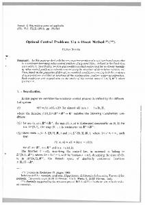
recommend to use a sum up rounding strategy as developed in [12], [14] in combination with a switching time optimization. Sum up rounding yields integer solutions arbitrarily close to the optimal integer solution, if a sufficiently fine time discretization is used. If guaranteed global solutions are an issue, this approach can be readily combined with methods in global optimization, of course. IV. N UMERICAL R ESULTS Numerical results have been computed with the optimal control software package MUSCOD-II [6]. For integration an adaptive fourth/fifth-order Runge-Kutta-Fehlberg method equipped with internal numerical differentiation (IND), cf. [1], was used. To solve the relaxed problem R t we apply homotopies, adding a regularization term ε · 0 f wδ2 (t) dt for the steering wheel angular velocity to the objective function and reducing ε down from 10, and doing a similar thing for the engine speed constraint. The computing time for each problem is well below two minutes on an AMD Athlon XP 3000+ with 2.166 GHz and 1024 MB of RAM. Parts of the optimal trajectory are shown in Figures 2 and 3. The optimal order of gears is (2, 3, 4, 3, 2, 1, 2, 3, 4, 3, 2, 1, 2). The gear switches take place after 1.87, 5.96, 10.11, 11.59, 12.21, 12.88, 15.82, 19.84, 23.99, 24.96, 26.10, and 26.76 seconds, respectively. The final time is tf = 27.7372 s.

(34)

This formulation has two main advantages. First, for many optimal control problems the optimal solution will have a bang–bang character, therefore the solution of the relaxed problem will yield the optimal integer solution. Second, for problems that fit into the class (33) a theory has been developed that allows to deduce information on the optimal integer solution from the optimal value of the relaxed problem, even if this solution is not bang–bang, but pathconstrained or sensitivity-seeking. See [12], [14] for theory and applications. D. Calculation of integer solutions Different methods for the calculation of integer solutions for mixed-integer optimal control problems, based on a direct approach, have been described and compared in [12]. Among them one finds Branch&Bound, Outer Approximation, penalization heuristics and rounding strategies. All methods that suffer from a combinatorial explosion when the number of discretized binary control variables increases have a very limited applicability, though. It can often be observed that the solution of the relaxed, purely continuous problem already yields an integer solution for almost all control discretizations. In addition, simple rounding strategies, taking the special ordered set constraint (33g) into account, often result in integer solutions without affecting the objective function value. For cases in which path-constraints play a role or a different objective function leads to sensitivity-seeking arcs, we

Fig. 2. The steering angle velocity (control), and some differential states of the optimal solution: directional velocity, side slip angle β, and velocity of yaw angle wz plotted over time. The vertical lines indicate gear shifts.

As can be seen in Fig. 3, the car uses the track width to its full extent, leading to active path constraints. As was expected, the optimal gear increases in an acceleration phase. When the velocity has to be reduced, a combination of braking, no acceleration, and engine brake is used. The result depends on the engine speed constraint reng (v(t), µ(t)) that becomes active in the braking phase. If the constraint is obmitted, the optimal solution switches directly from the fourth gear into the first one to maximize

1567

47th IEEE CDC, Cancun, Mexico, Dec. 9-11, 2008

TuC10.5

Gear 4 Gear 3

50

Gear 3

y [m]

Gear 2 Gear 1 0

Gear 2 Initial Positions

Gear 2

Gear 1 Gear 2 Gear 3

-50

Gear 3

-150

-100

Gear 4

-50

0 x [m]

50

100

150

Fig. 3. Elliptic race track seen from above with optimal position and gear choices of the car. Note the exploitation of the slip (sliding) to change the car’s orientation as fast as possible, when in first gear. The gear order changes when a different maximum engine speed is imposed.

the effect of the engine brake. For nMAX eng = 15000 braking occurs in the gear order 4, 2, 1. Although this was left as a degree of freedom, the optimizer yields a symmetric solution with respect to the upper and lower parts of the track for all scenarios we considered. V. C ONCLUSIONS We reformulated and extended a recently published benchmark problem in mixed-integer optimal control. With a solution approach based on an outer convexification and a relaxation of the integer constraints we obtained periodic solutions on an elliptic track without any a priori assumptions on the switching structure. The approach is generic and is also applicable to different car models, tracks, and to other objectives, e.g., energy optimality. The tremendous speedup compared to previous approaches allows for an extension to more realistic racing tracks and models, and to nonlinear model predictive control of switched systems. R EFERENCES [1] I. Bauer, H.G. Bock, and J.P. Schl¨oder. DAESOL – a BDF-code for the numerical solution of differential algebraic equations. Internal report, IWR, SFB 359, Universit¨at Heidelberg, 1999. [2] T. Binder, L. Blank, H.G. Bock, R. Bulirsch, W. Dahmen, M. Diehl, T. Kronseder, W. Marquardt, J.P. Schl¨oder, and O.v. Stryk. Introduction to model based optimization of chemical processes on moving horizons. In M. Gr¨otschel, S.O. Krumke, and J. Rambau, editors, Online Optimization of Large Scale Systems: State of the Art, pages 295–340. Springer, 2001. [3] H.G. Bock. Numerical treatment of inverse problems in chemical reaction kinetics. In K.H. Ebert, P. Deuflhard, and W. J¨ager, editors, Modelling of Chemical Reaction Systems, volume 18 of Springer Series in Chemical Physics, pages 102–125. Springer, Heidelberg, 1981.

[4] H.G. Bock and R.W. Longman. Computation of optimal controls on disjoint control sets for minimum energy subway operation. In Proceedings of the American Astronomical Society. Symposium on Engineering Science and Mechanics, Taiwan, 1982. [5] H.G. Bock and K.J. Plitt. A multiple shooting algorithm for direct solution of optimal control problems. In Proceedings 9th IFAC World Congress Budapest, pages 243–247. Pergamon Press, 1984. [6] M. Diehl, D.B. Leineweber, and A.A.S. Sch¨afer. MUSCOD-II Users’ Manual. IWR-Preprint 2001-25, Universit¨at Heidelberg, 2001. [7] M. Gerdts. Solving mixed-integer optimal control problems by branch&bound: A case study from automobile test-driving with gear shift. Optimal Control Applications and Methods, 26:1–18, 2005. [8] M. Gerdts. A variable time transformation method for mixed-integer optimal control problems. Optimal Control Applications and Methods, 27(3):169–182, 2006. [9] C. Kirches, S. Sager, H.G. Bock, and J.P. Schl¨oder. Time-optimal control of automobile test drives with gear shifts. Optimal Control Applications and Methods, 2009. (submitted). [10] D.B. Leineweber, I. Bauer, A.A.S. Sch¨afer, H.G. Bock, and J.P. Schl¨oder. An efficient multiple shooting based reduced SQP strategy for large-scale dynamic process optimization (Parts I and II). Computers and Chemical Engineering, 27:157–174, 2003. [11] H.B. Pacejka and E. Bakker. The magic formula tyre model. Vehicle System Dynamics, 21:1–18, 1993. [12] S. Sager. Numerical methods for mixed–integer optimal control problems. Der andere Verlag, T¨onning, L¨ubeck, Marburg, 2005. ISBN 3-89959-416-9. Available at http://sager1.de/sebastian/downloads/Sager2005.pdf. [13] S. Sager, M. Diehl, G. Singh, A. K¨upper, and S. Engell. Determining SMB superstructures by mixed-integer control. In K.-H. Waldmann and U.M. Stocker, editors, Proceedings OR2006, pages 37–44, Karlsruhe, 2007. Springer. [14] S. Sager, G. Reinelt, and H.G. Bock. Direct methods with maximal lower bound for mixed-integer optimal control problems. Mathematical Programming, published online at http://dx.doi.org/10.1007/s10107-007-0185-6 on 14 August 2007, 2008. [15] J. Till, S. Engell, S. Panek, and O. Stursberg. Applied hybrid system optimization: An empirical investigation of complexity. Control Eng, 12:1291–1303, 2004.

1568