tionary learning [2, 5] and compressive sensing [8, 9, 13], among others. Given a set of basis vectors (i.e., a dictio- nary), finding a sparse representation of a ...
Fast Sparse Representation with Prototypes Jia-Bin Huang and Ming-Hsuan Yang University of California at Merced {jbhuang,mhyang}@ieee.org
Abstract Sparse representation has found applications in numerous domains and recent developments have been focused on the convex relaxation of the `0 -norm minimization for sparse coding (i.e., the `1 -norm minimization). Nevertheless, the time and space complexities of these algorithms remain significantly high for large-scale problems. As signals in most problems can be modeled by a small set of prototypes, we propose an algorithm that exploits this property and show that the `1 -norm minimization problem can be reduced to a much smaller problem, thereby gaining significant speed-ups with much less memory requirements. Experimental results demonstrate that our algorithm is able to achieve double-digit gain in speed with much less memory requirement than the state-of-the-art algorithms.
1. Introduction Recent years have witnessed a considerable resurgence of interest in sparse representation [27, 21, 5]. Much of its popularity as well as effectiveness come from the fact that signals in most problems are structured and can be well represented by a small set of basis vectors. It plays an important role in the success of recent developments in dictionary learning [2, 5] and compressive sensing [8, 9, 13], among others. Given a set of basis vectors (i.e., a dictionary), finding a sparse representation of a signal is often posed as an optimization problem with either `0 -norm or `1 norm, which usually results in solving an underdetermined linear system. Each sample is then represented as a sparse linear combination of the basis vectors. The complexity of solving `0 -norm minimization problems is known to be NP-hard and numerically unstable. Greedy algorithms such as matching pursuit [25], and orthogonal matching pursuit (OMP) [10, 29] have been proposed to approximate the `0 norm solution. Although these methods are rather simple and efficient, the solutions are sub-optimal. Recent developments in sparse coding have shown that, under certain assumptions, the solution of `0 -norm minimization problem is equivalent to `1 -norm minimization problem which can be solved by convex optimization [11, 13]. Numerous algo-
rithms have been proposed for `1 -regularized sparse coding [7, 8, 9, 13, 12, 32]. As these algorithms often recast the original problem as a convex program with quadratic constraints, the computational cost for practical applications can be prohibitively high. For numerous problems in computer vision, machine learning, signal processing, and computer graphics, one simple yet effective approach is to assume that the samples of the same class can be modeled with prototypes or exemplars. Such prototypes can be either the samples themselves, or learned from a set of samples (e.g., eigenvectors and means from vector quantization). Examples abound. In visual processing, it has been shown that prototypical models are capable of capturing intra-class variations such as appearance [26] and lighting [3]. In graphics, prototypes are learned from images and utilized for synthesizing videos for animation [16]. Prototypical representations have also been exploited in signal processing, clustering, dimensionality reduction, dictionary learning compressive sensing, visual tracking and motion analysis , to name a few [5]. In this paper, we assume that samples from one class can be modeled with a small set of prototypes from the same class. Among the above-mentioned prototype learning algorithms, the method of optimal directions (MOD) [15] and K-SVD algorithms [14] are of great interest as they are able to represent each sample with a sparse combination of dictionary atoms or prototypes. Assuming that we are given a learned dictionary, we can first approximate the basis vectors with sparse representation using the prototypes in this dictionary. As will be explained later in this paper, the original sparse representation problem can then be reduced to a much smaller problem with `1 -norm constraints. By exploiting the linear constraints of these prototypes and basic concepts in linear algebra, we show that the original `1 norm minimization problem can be reduced from a large and dense linear system to a small and sparse one, thereby obtaining significant speed-up. We apply the proposed algorithm to several large data sets and demonstrate that it is able to achieve double-digit gain in speed with much less memory requirement than the state-of-the-art sparse coding methods.
2. Sparse Representation with Prototypes In numerous problems we are often given a set of labeled samples for each class and the goal is to correctly infer the class of unseen samples by using the knowledge learned from the given samples. Suppose that we collect ni samples from the i-th of K distinct signal classes, we define a matrix Φi ∈ IRm×ni for class i as columns of samples: Φi = [φi,1 , φi,2 , · · · , φi,ni ],
(a)
(b)
(1)
where φi,j ∈ IRm stands for the j-th sample of the class i. We then concatenate all samples for all K classes into a matrix Φ ∈ IRm×N : Φ = [Φ1 , Φ2 , · · · , ΦK ],
(2)
where N is the total number of samples from all classes. Given a sufficient number of samples for class i, an observed sample y can be well approximated by a linear combination of the samples if y belongs to class i: y = ci,1 φi,1 + ci,2 φi,2 + · · · + ci,ni φi,ni ,
(3)
where the scalar ci,j represents the weighted contribution of the j-th sample in reconstructing the observed sample y. However, we do not know which class the sample y belongs to in most circumstances. Thus, we can rewrite the linear representation of y using all samples compactly as: y = Φx,
(4)
where x = [0, · · · , 0, ci,1 , · · · , ci,ni , 0, · · · , 0]> is a sparse coefficient vector. Usually, Φ is a fat and dense matrix as illustrated in Figure 1(a).
(c)
samples from that class. Such property has been exploited extensively in the literature, e.g., local linear embedding, image clustering, spectral methods, and face recognition [5]. With a sufficiently large number of samples for each class, the coefficient vector x is expected to be very sparse, i.e., only a small portion of entries are nonzero. Regularized via sparsity constraints, we seek a representation for an observed sample y: min kxk0 subject to y = Φx,
2.1. Solving Inverse Linear System
x
With the formulation in (4), each observed sample y can be represented with the corresponding coefficient vector x by solving the linear system y = Φx. If the dimension of the observation data y is larger than the number of all samples (i.e., m > N ), then the unique solution can usually be obtained by solving the overdetermined system. However, in most applications, the linear systems are ill-conditioned or underdetermined, resulting in infinitely many solutions to this inverse problem (as shown in Figure 1(a)). Therefore, regularization constraints are of critical importance for obtaining useful solutions. For example, solutions can be obtained by solving the following minimum `2 -norm problem: min kxk2 subject to y = Φx, x
(d)
Figure 1. Sparse representation algorithms. (a) The original problem that solves y = Φx where Φ is a dense fat matrix. (b) The proposed method solves wey = Wx where W is a tall sparse matrix. (c) The proposed method further reduces W to a tall skinny matrix WR and solves wey = WR xR . (d) The proposed method reduces the matrix W to a tall skinny matrix WR with relaxed constraints and solves wey = WR xR .
(5)
and the minimum `2 -norm solution can be obtained by ˆ x2 = (ΦT Φ)−1 ΦT y. However, the minimum `2 -norm solution ˆ x2 is usually dense (i.e., with many nonzero entries), thereby losing the discriminative ability to select the most relevant samples for representing the observed sample y. Since an observed sample is assumed to belong to one certain class, it can usually be well represented using other
(6)
where k · k0 : IRN → IR counts the number of nonzero entries. However, solving the `0 -norm minimization of an underdetermined system is both numerically unstable and NP-hard [5]. Recently, theories developed from sparse representation and compressive sensing [8, 9, 13] suggest that if the solution of x is sparse enough, then the sparsest solution can be recovered via the `1 -norm minimization: min kxk1 subject to y = Φx, x
(7)
where the `1 -norm sums up the absolute weights of all entries in x. Note that the equality constraint in (7) can be relaxed to allow small noise, and the sparest solution x0 can be approximately recovered by finding the minimum `1 -norm vector, x, that best explains the observed sample y: min kxk1 subject to ky − Φxk2 ≤ �, x
(8)
where � is the allowed error tolerance. The problems of solving (7) and (8) are convex programs which can be solved by recasting them as linear programs (LP) and second-order cone programs (SOCP) [7, 5], respectively.
2.2. Feature Extraction by Linear Transformation Since directly operating on the original space of image observations is computationally expensive due to extremely high data dimensions, numerous feature extraction methods have been proposed to project the original data onto a low dimensional feature space. Thanks to the fact that most feature extraction methods require or can be approximated by linear transformations, the mapping from the image observation space to the feature space can be characterized by a matrix T ∈ IRd×m , where d Φ and WR > WR [4]. Thus, the time complexity of the matrix multiplication for a dense matrix Φ and WR is O(m2 N 2 ) flops and O(L2 NR2 ) flops, respectively. The time complexity ratio between the original and proposed method is mainly determined by the quadratic terms, 2 N2 N2 i.e., O( L2 N 2 +dLNm 2 +dL+LN ) ≈ O( N 2 ), as NR is +LN R R R R much smaller than N , and L and m are usually of the same scale. As a result, the proposed algorithm achieves significant quadratic speed-up. In the intermediate step, the space complexity of the proposed algorithm for storing the learned dictionary and basis matrix W of (12) is O(LK + KN ). However, the space complexity for the reduced matrix wey is O(NR ). As the quadratic constraints of Φ> Φ and WR > WR are computed in solving `1 -minimization, the original formulation again has much higher space complexity than the proposed one, N2 N2 with the ratio of O( LK+KN ) ≈ O( N 2 ). +N 2 R
R
4. Experimental Results In this section, we present experimental results on both synthetic and real data sets to demonstrate the efficiency and effectiveness of the proposed algorithm. All the experiments were carried out using MATLAB implementations to solve the original and proposed relaxed `1 -norm minimization problems described in Section 2.2 as well as Section 3.3 on a 1.8 GHz machine with 2 GB RAM. The MATLAB code and processed data is available at faculty.ucmerced.edu/mhyang/fsr.html.
4.1. Synthetic Data We validate the effectiveness of sparse representations and the efficiency of the proposed approximation for signal classification in the presence of Gaussian white noise. We first build a dictionary with all elements drawn from a Gaussian random variable with zero mean and unit variance. The columns of the dictionary are then normalized to unit norm. Since samples from one specific class are assumed to lie in certain subspace that can be modeled by prototypes, we generate samples by first selecting five columns in the dictionary and then obtain each sample by a linear combination of the selected columns. In the first experiment, we generate 50 samples for each of the 10 classes, where the dimension of each sample is 25. The test samples, assumed to lie in one unknown subspace, are generated by randomly selecting one signal class and combining three training samples from the selected class with random coefficients. Gaussian noise of different levels are added to the test samples for experiments. We generate 100 test samples to evaluate the recognition capability of the classification based on sparse representation. That is, for each test sample, we need to solve (10) with matrix F ∈ IR25×500 for recognition (using their sparse coefficients to find the class with minimum reconstruction error). In this experiment, we use the K-SVD algorithm to learn the underlying dictionary D ∈ IR25×100 from F although other algorithms such as MOD can be substituted. In the sparse coding stage, OMP with sparsity factor 5 (i.e., the maximum allowed nonzero coefficients) is used. After 10 iterations of the dictionary learning process, we compute the sparse representations of samples in F and ˜y. With these sparse representations, we can obtain the approximated solution of x by solving (18). In Figure 2, we report the recognition rates of methods with sparse representation from solving (10) and (18) where the label is determined based on minimum reconstruction error. It shows that these methods are able to recognize correct classes even under substantial noise corruption (up to 20%). Furthermore, the classifier with the proposed algorithm (using (18)) achieves higher recognition rate than the one with original one (using (10)). This is because that when samples in F are coded with sparse representation using dictionary D, noise in the signals are also removed as a by-product of `1 -norm minimization. In the second synthetic experiment, we present the runtime performance of the proposed method and the state-ofart `1 -norm optimization solver with SOCP techniques [7]. We increase both the number of signal class and the feature dimension of samples to 50. Following similar procedure as described in the first experiment, we generate three sets of training samples (500, 1000, 1500). Like the previous experiment, 100 test samples are obtained in the same way as previous setting with noise of zero mean and σ 2 is set to 0.1. Table 1 shows the mean value of the recognition rates
Table 1. Comparison on recognition speed and accuracy using synthetic data sets. Sample size 500 1000 1500 Method Acc (%) Time (s) Acc (%) Time (s) Acc (%) Time (s) Original 96.0 0.7575 96.6 4.4548 97.0 12.3191 Proposed 93.0 0.0061 94.6 0.0114 96.0 0.0217 Speed-up 124.2 390.8 567.7
Figure 2. Recognition rates of the original and the proposed algorithm in signal classification task with the presence of noise.
and the average computation time per test sample needed in solving these two equations. Although the classifier with sparse representation obtained by the original l1 -norm minimization has slightly higher recognition rate in this setting, however, the execution time increases rapidly as the number of the samples increases. On the other hand, the classifier with the proposed algorithm achieves comparable results in accuracy but with significant speed-up. For the set of 1500 samples, our method solves the l1 -norm minimization problem 567.7 times faster than the l1 -magic solver (using log barrier algorithm for SOCP) [7]. The reason that the proposed method achieves slightly worse results in accuracy may result from the imperfect approximation of the sparse approximation using the K-SVD algorithm. We note that this is a trade-off between accuracy and speed that can be adjusted with parameters in the K-SVD algorithm (e.g., the number of coefficients in OMP). It is also worth noticing that l1 -magic solver can handle up to 4500 data points (of 50 dimensions) whereas our algorithm is able to handle more than 10000 data points.
4.2. Face Recognition We use the extended Yale database B which consists of 2414 frontal face images of 38 subjects for experiments [20]. These images were acquired under various lighting conditions and normalized to canonical scale (as shown in Figure 3). For each subject, we randomly select half of the images as training samples and use the rest for tests.
Figure 3. Sample images from the extended Yale database B.
Since the original data dimension is very high (192 × 168 = 32256), we use two feature extraction methods (downsampling and PCA) to reduce their dimensionality (i.e. difference choice of T in (9)). In the appearancebased face recognition setup each image is downsampled to 12 × 11 pixels (i.e., d = 132). For PCA, we compute the eigenfaces using the training images and retain the coefficients of the largest 132 eigenvectors. A dictionary of size 132 × 264 (i.e., redundancy factor of 2) is trained using the K-SVD algorithm with 10 iterations. For each sample, at most 10 coefficients are used for sparse coding with OMP. As shown in Table 2, the proposed algorithm achieves comparable recognition rates but with significant speedup. Note that the required time to classify one image using the original l1 -norm minimization is more than 20 seconds, which makes it infeasible for real-world applications. By increasing the redundancy of the dictionary or reducing the maximum allowed number of coefficients for in representing an image (i.e., making the representation even more sparser), we can achieve more speed-ups at the expense of slight performance degradation. Table 2. Recognition accuracy and speed using the Extended Yale database B. Feature Downsampled image PCA Method Acc (%) Time (s) Acc (%) Time (s) Original 93.78 20.08 95.01 13.17 Proposed 91.62 0.51 92.28 0.32 Speed-up 39.4 41.2
4.3. Single Image Super-Resolution We apply the proposed algorithm to image super resolution using sparse representation [34], which assumes sparsity prior for patches from a high-resolution image. Two dictionaries, one for the low-resolution image and the other for the high-resolution one, are trained using patches randomly selected from an image collection. The reconstructed high resolution image can then be obtained by solving `1 norm penalized sparse coding. Here the original `1 -norm penalized sparse coding adopted is based on the efficient sparse coding algorithm in [19]. The dictionary size is set 6 times the feature dimensions in the low-resolution dictionary. For each sample, 3 coefficients are used for spare approximation by OMP. In Table 3, we report the root-mean-square error (RMSE) values in pixel intensity and the execution time of sparse
coding for all patches on four test images used in [34]: Girl, Flower, Panthenon, and Racoon. The proposed algorithm achieves double-digit speedups with slight performance degradation (in terms of RMSE). However, the RMSE measure is not the best metric for super resolution as it does not directly reflect the visual quality and oftentimes we do not have ground truth high-resolution images. Figure 4 shows visual quality of the proposed algorithm is much better than the results using bicubic interpolation, and very similar to the results of [34]. Table 3. Execution time and RMSE for sparse coding on four test images (scale factor = 3) Image Method Girl Flower Panthenon Racoon
Original [19] RMSE Time (s) 5.6684 17.2333 3.3649 14.9173 12.247 35.1163 9.3584 27.9819
Proposed RMSE Time (s) 6.2837 1.5564 3.8710 1.3230 13.469 3.1485 10.148 2.3284
Speedup 11.07 11.27 11.15 12.02
Figure 5. Sample images from the INRIA data set [1].
For each test image, we find the sparse representation by solving the l1 -norm minimization problem. That is, the resulting linear combination of training images best represent the test image with minimum reconstruction error (in `2 -norm). The estimated pose of the test image is then computed by the same linear combination of the associated pose parameters in the training set. We report in Table 4 the execution time of solving the l1 norm minimization problem with different numbers of prototypes. We note that the mean estimation error of 3D joint angles decreases as the number of prototypes is increased. Overall, the speed can be improved significantly with only slight performance degradation.
4.5. Multi-View Object Recognition
(a)
(b)
(c)
(d)
Figure 4. Image super-resolution visual results. (a) Ground-truth high resolution image. (b) Bicubic interpolation. (c) Superresolution via sparse representation [34]. (d) Proposed method.
4.4. Human Pose Estimation We apply the sparse representation to the problem of estimating human pose from single images. Here we pose this problem as a regression that maps image observations to three-dimensional joint angles. In training set, we are given a number of silhouette images and their corresponding pose parameters. The task is to infer the three-dimensional human pose of an unseen test image. We validate the applicability of the sparse representation to this regression problem and demonstrate the improvement in speed with the proposed algorithm. We use the INRIA data set [1] in which 1927 silhouette images are used for training and 418 images for tests (some samples are shown in Figure 5). The image descriptors we use are the 100-dimensional feature vectors (i.e., histogram of shape context descriptors) as computed in [1].
We compare the proposed method against the original algorithm using the Columbia Object Image Library (COIL100) data set [26]. The COIL-100 data set has been widely used in object recognition literature, and it consists of color images of 100 distinct objects; 72 images of each object placed on a turntable were captured at pose interval of 5 degrees. Typically, a few number of images from different views with constant interval are selected as training samples and the others are used for tests. For example, if 18 views are selected from each object class for experiments, there will be 1800 training and 5400 test images. The 128 × 128 images are first converted to gray images and then downsampled to 32 × 32 pixels. Two kinds of simple features (downsampled image and PCA) are used for evaluations. Meanwhile, two different feature dimensions are used for experiments. The dictionary size is set 4 times the feature dimensions (i.e., 4d). For each sample, 3 coefficients are used for spare representation by OMP. The recognition rate and the average execution time for processing one sample are summarized in Table 5. Overall, the proposed algorithm achieves about 10000 times faster than the original method with comparable accuracy (note the execution time are recorded in different scales).
5. Conclusion In this paper, we have presented a fast sparse representation algorithm that exploits the prototype constraints inhere in signals. We show that sparse representation with `1 -norm minimization can be reduced to a smaller linear system and thus significant gains in speed can be obtained. In addition, the proposed algorithm requires much less memory than the state-of-the-art `1 -minimization solver. Experimental
Table 4. Comparison on pose estimation accuracy and speed under different number of prototypes using the INRIA data set. Number of coefficients 3 6 9 12 15 Original l1 -norm minimization Mean error (in degrees) 9.1348 7.9970 7.4406 7.2965 7.1872 6.6513 Execution time (in seconds) 0.0082 0.0734 0.3663 1.1020 2.3336 24.69 Speed-up 3011.0 336.4 67.4 22.4 10.6 Table 5. Comparison on recognition speed and accuracy on the COIL-100 (note some values are listed in different scales). Number of view Feature used Downsampling(16 × 16) Downsampling(10 × 10) PCA: 256 PCA: 100
8 Orig. (%) 82.43 75.08 84.56 81.23
16 Recognition accuracy Ours (%) Orig. (%) 80.93 90.01 74.28 84.75 82.08 91.03 79.23 90.58
8 Ours (%) 87.43 84.00 89.22 87.72
results on several image and vision problems demonstrate that our algorithm is able to achieve double-digit gain in speed with much less memory requirement and comparable accuracy. Our future work will focus on extending the proposed fast algorithm for learning discriminative sparse representations for classification problems. We are also interested in analyzing the interplay between RIP assumption and the effectiveness of the proposed method. As the proposed algorithm is able to handle large-scale data collections, we will explore other real-world applications such as image search and visual tracking.
Acknowledgments The authors would like to thank anonymous reviewers for their comments. This work is partially supported by a UC Merced faculty start-up fund and a gift from Google.
References [1] A. Agarwal and B. Triggs. Recovering 3d human pose from monocular images. IEEE Transactions on Pattern Analysis and Machine Intelligence, 28(1):44–58, 2006. 7 [2] M. Aharon, M. Elad, and A. Bruckstein. K-SVD: An algorithm for designing overcomplete dictionaries for sparse representation. IEEE Transactions on Signal Processing, 54(11):4311, 2006. 1, 3 [3] P. N. Belhumeur and D. J. Kriegman. What is the set of images of an object under all possible illumination conditions. International Journal of Computer Vision, 28(3):1–16, 1998. 1 [4] S. Boyd and L. Vandenberghe. Convex optimization. Cambridge university press, 2004. 5 [5] A. Bruckstein, D. Donoho, and M. Elad. From sparse solutions of systems of equations to sparse modeling of signals and images. SIAM Review, 51(1):34– 81, 2009. 1, 2, 3, 5 [6] O. Bryt and M. Elad. Compression of facial images using the K-SVD algorithm. Journal of Visual Communication and Image Representation, 19(4):270–282, 2008. 3 [7] E. Candes and J. Romberg. `1 -magic; Recovery of sparse signals via convex programming. California Institute of Technology, 2005. http://www.acm.caltech.edu/l1magic/. 1, 2, 5, 6 [8] E. Cand`es, J. Romberg, and T. Tao. Stable signal recovery from incomplete and inaccurate measurements. Communications on Pure and Applied Mathematics, 59:1207–1223, 2006. 1, 2 [9] E. Candes and T. Tao. Near-optimal signal recovery from random projections: Universal encoding strategies? IEEE Transactions on Information Theory, 52(12):5406–5425, 2006. 1, 2, 4 [10] S. Chen, S. Billings, and W. Luo. Orthogonal least squares methods and their application to non-linear system identification. International Journal of Control, 50(5):1873–1896, 1989. 1 [11] S. Chen, D. Donoho, and M. Saunders. Automatic decomposition by basis pursuit. SIAM Journal of Scientific Computation, 20(1):33–61, 1998. 1, 3 [12] D. Donoho and Y. Tsaig. Fast solution of `1 -norm minimization problems
Orig. (s) 6.85 4.13 3.71 2.54
[13] [14] [15] [16] [17] [18] [19] [20] [21] [22] [23] [24] [25] [26] [27] [28] [29]
[30] [31] [32] [33] [34]
Ours (ms) 3.2 3.9 3.3 3.6
16 Execution time Speed-up Orig. (s) 2140.6 52.73 1059.0 48.02 1124.2 29.58 705.6 21.00
Ours (ms) 3.9 5.2 3.8 5.6
Speed-up 13520.5 9234.6 7784.2 3750.0
when the solution may be sparse. IEEE Transactions on Information Theory, 54(11):4789–4812, 2008. 1, 5 D. L. Donoho. For most large underdetermined systems of linear equations the minimal `l -norm solution is also the sparsest solution. Communications on Pure and Applied Mathematics, 59(6):797–829, 2006. 1, 2, 3 M. Elad and M. Aharon. Image denoising via sparse and redundant representations over learned dictionaries. IEEE Transactions on Image Processing, 15(12):3736–3745, 2006. 1, 3 K. Engan, S. O. Aase, and J. H. Husoy. Method of optimal directions for frame design. In Proceedings of the IEEE International Conference on Acoustics, Speech, and Signal Processing, pages 2443–2446, 1999. 1, 3 T. Ezzat, G. Geiger, and T. Poggio. Trainable videorealistic speech animation. In Proceedings of ACM SIGGRAPH, pages 388–398, 2002. 1 K. Huang and S. Aviyente. Sparse representation for signal classification. In NIPS, volume 19, pages 609–616, 2006. 3 K. Kreutz-Delgado, J. F. Murray, B. D. Rao, K. Engan, T. W. Lee, and T. J. Sejnowski. Dictionary learning algorithms for sparse representation. Neural Computation, 15(2):349–396, 2003. 3 H. Lee, A. Battle, R. Raina, and A. Y. Ng. Efficient sparse coding algorithms. pages 801–808, 2006. 6, 7 K.-C. Lee, J. Ho, and D. J. Kriegman. Acquiring linear subspaces for face recognition under variable lighting. IEEE Transactions on Pattern Analysis and Machine Intelligence, 27(5):684–698, 2005. 6 M. S. Lewicki and T. J. Sejnowski. Learning overcomplete representations. Neural Computation, 12(2):337–365, 2000. 1, 3 J. Mairal, F. Bach, J. Ponce, G. Sapiro, and A. Zisserman. Discriminative learned dictionaries for local image analysis. In Proceedings of IEEE Conference on Computer Vision and Pattern Recognition, 2008. 3 J. Mairal, M. Elad, and G. Sapiro. Sparse representation for color image restoration. IEEE Transactions on Image Processing, 17(1):53, 2008. 3 J. Mairal, G. Sapiro, and M. Elad. Learning multiscale sparse representations for image and video restoration. SIAM Multiscale Modeling and Simulation, 7(1):214–241, 2008. 3 S. G. Mallat and Z. Zhang. Matching pursuits with time-frequency dictionaries. IEEE Transactions on Signal Processing, 41(12):3397–3415, 1993. 1 H. Murase and S. Nayar. Visual learning and recognition of 3-D objects from appearance. International Journal of Computer Vision, 14(1):5–24, 1995. 1, 7 B. A. Olshausen and D. J. Field. Emergence of simple-cell receptive field properties by learning a sparse code for natural images. Nature, 381(6583):607–609, 1996. 1, 3 B. A. Olshausen and D. J. Field. Sparse coding with an overcomplete basis set: A strategy employed by V1? Vision Research, 37(23):3311–3325, 1997. 3 Y. C. Pati, R. Rezaiifar, and P. S. Krishnaprasad. Orthogonal matching pursuit: Recursive function approximation with applications to wavelet decomposition. In Conference Record of The Twenty-Seventh Asilomar Conference on Signals, Systems, and Computers, pages 40–44, 1993. 1 D. Pham and S. Venkatesh. Joint learning and dictionary construction for pattern recognition. In Proceedings of IEEE Conference on Computer Vision and Pattern Recognition, 2008. 3 R. Rubinstein, M. Zibulevsky, and M. Elad. Efficient implementation of the k-svd algorithm using batch orthogonal matching pursuit. Technical Report CS-2008-08, Technion, 2008. 5 J. A. Tropp and S. J. Wright. Computational methods for sparse solution of linear inverse problems. Technical Report 2009-01, California Institute of Technology, 2009. 1, 3, 5 J. Wright, A. Yang, A. Ganesh, S. Sastry, and Y. Ma. Robust face recognition via sparse representation. IEEE Transactions on Pattern Analysis and Machine Intelligence, 31(2):210–227, 2009. 3 J. Yang, J. Wright, T. Huang, and Y. Ma. Image super-resolution as sparse representation of raw image patches. In Proceedings of IEEE Conference on Computer Vision and Pattern Recognition, 2008. 3, 6, 7


![UC Merced Campus Profile - UC Merced Institutional Planning ... [PDF]](https://m.moam.info/img/260x300/uc-merced-campus-profile-uc-merced-institutional-p_64a22ba6098a9e43608b45d6.jpg)