weighted residual sum of squares (WKSS) of the three models are very close, other criteria should be used to determine the best fit model. Compare Model.
1996 IEEE E N C O N - Digital Signal Processing Applications
Fast System Identification Algorithm for Non-uniformly Sampled Noisy Biomedical Signal Koon-Pong Wong Dagan Feng * , and Wan-Chi Siu
'
'
Department of Electronic Engineering The Hong Kong Polytechnic University, Hung Hom, Kowloon, Hong Kong Baser Department of Computer Science The University of Sydney, N.S.W. 2006, Australia
ABSTRACT - The recently developed generalized linear least squares (GLLS) algorithm has been found v e v useful in non-uniformly sampled biomedical signal processing and parameter estimation. In this paper, the algorithm is used for the identification of a compartmental model with a pair of repeated eigenvalues bused on the nonuniformly sampled noisy data. A ca,re study is presented, which demonstrates that the algorithm is able to select the most suitable model for the system from the non-uniformly sampled noisy signals.
I. INTRODUCTION System identification is generally referred to as the determination of a mathematical rnodel for a system or a process by observing the input-output relationships. In biomedical system identification, the key issue is to estimate the physiological parameters of a model based on the sampled data from a dynamic process. This model can usually be described by a set of differential equations. If the data can be sampled uniformly as in most of the engineering systems, the indirect method can be utilized and the signal processing is relatively straightforward. The indirect method proceeds by first estimating the parameters for a discrete-time model that best fits the data at these uniformly sampled times. The discrete-time model parameters are subsequently converted into the parameters of an equivalent continuous-time model through ImpulseInvariance method, which guarantees that the continuous-time and discrete-time models have identical output values at these uniformdy sampled instances. The advantage of using the indirect method is that a number of effective parameters estimation algorithms are available, e.g. Least Squares (LS), Instrumental Variable (IV), Multistage Least Squares, and Generalized Least Squares (GLS) [6]. Among these methods, GLS has the highest accuracy. GLS iteratively upgrades the estimates that are initially obtained from the Least Squares and the final estimates are unbiased. However, in contrary to engineering systems, the dynamic data in most biomedical systems are usually
sampled non-uniformly [7]. In these cases, the welldeveloped indirect method algorithms cannot be used. The direct method, on the other hand, estimates the continuous-time rnodel parameters by fitting these non-uniformly sampled data directly. The classic nonlinear least squares (NLS) is widely applied and can provide parameter estimates of optimum statistical accuracy [lo]. Nevertheless, good initial parameter values are required and the computational complexity of this algorithm is very high. If the initial parameter values are not close enough to the parameter true values, NLS will converge very slowly or even not converge at all. Other algorithms such as System Reference Adaptive Model, Maximum Likelihood (ML), and Prediction Error [2] are all very time-consuming. As a result, they are impractical for high resolution image-wide parameter estimation. Recently, Feng et a1 [ 5 ] proposed an Generalized Linear Least Squares (GLLS) algorithm for parameter estimation of non-uniformly sampled biomedical systems. This algorithm can provide unbiased parameter estimation with very little computing time and without the need of providing the initial parameter values. As it is statistically reliable and computationally efficient, it has been found to be very useful for biomedical system identification and image-wide parameter estimation [4,5]. However, this algorithm cannot deal with the signals and systems containing repeated eigenvalues which often occur in biological systems [3]. Wong et a1 [9] extended it so that it can be used for identification of system containing repeated eigenvalues as well. In this paper, the GLLS algorithm is used for the identification of a compartment model and the case study demonstrates that the algorithm is able to select the suitable model for the system based on the non-uniformly sampled data.
11. THEORY The general Single-Input-Single-Output (SISO) linear continuous dynamic system can be described by the following n-th order differential equation:
559 0-7803-3679-8/96/$5.000 1996 IEEE
Authorized licensed use limited to: Hong Kong Polytechnic University. Downloaded on June 25,2010 at 04:06:09 UTC from IEEE Xplore. Restrictions apply.
y'll'(t> + aly("-')(t)+ . .. + a,y(t)
= blu'"-''(t)
+ bzu'n-2)(t)+ ...+ b,u(t)
convenience, we denote the number of the parameters to be estimated as p. Integrating equation (6) n times from 0 to t, (i=1,2,...,m) with respect to t, we get the following matrix equation
(1)
where u(t) and y(t) are the input and output of the system respectively, al, az, ... , a, and bl, b2, ... ,b, are the system transfer function parameters. The Laplace transform of equation (1) is given by S"Y(S) -
s"-'y(o) - ... - y'""'(o)
-t al[s"-'Y(s)
y=X8+5
- S"-~Y(O)
2'(~)1 -t ... + a,Y(s) = bl[s"-'U(s) - s"?I(O)-...- u'"-~'(O)]+...+ b,U(s) - ... - y'"
(2)
(7)
where y=[y(tl), y(t2), _ _ _ , y(tm)lTis the column vector of the measurements at times tl, tz, ..., t,, and 8=[-al, ..., -a,, bl, ..., b,, v1, ..., v, IT is the column vector of the parameters to be estimated with dimension of p, X is the m x p coefficient matrix containing integrals of input or output, or functions oft:
where u(O), .._ u'"-~'(O)and y(O), ".. , y'""'(0) are the initial conditions for the input and output functions. Equation (2) can be rewritten as ~
(SI'
+ ... + a,)Y(s) = (bls"-' + b2sn-2 + "..-+ bn)U(s)+ visn-' + v2sn-' + ... +
ialsn-'
v,
(3)
5=
[ c l , 52, ... cm]' is the column vector of the equation noise terms. These terms originate from the measurement noise in y(t). If m = p and X-' exists, we can solve 0 uniquely from equation (7) by
where vl, v2, ... v, are the linear combinations of the input and output initial conditions, with al, ... , a, and bl, ... , b, as their coefficients. vi (i = 0, 1, 2, ... , n) can be written in matrix form as below: ~
0=X-'y
(8)
6
where denotes the estimate of 8. If m > p, the linear least squares (US) solution for 0 is given by, Let A(s) = S" + alsn-' -+ ... -+ a, , B(s) = bls"-i + b2sn-2 -+ ... + b, and V(s) = v1sn-' + v2sn-' + ... -+ v,. Equation (3) is further abbreviated as:
A(s)Y(s) = B(s)U(s) + V(s)
(4)
In most of the cases, the initial conditions are all zeros. If some of the initial conditions are unknown, they can be considered as the unknown parameters to be estimated. Dividing both sides of equation (3) by s" and rearranging it, we get
6U-s
= (XTX)-'XTy
(9)
where represents the estimated 8 in the linear lease squares sense. The estimates from equation (9) are biased, even though the direct measurement noise is white or independent at different sampling times [5,9]. In other words, the equation noise 6 is correlated or coloured. This can also be shown in the frequency domain as follows. If we rearrange equation (4) and add a white measurement noise term to the equation, we have
Y(s) = -als-'Y(s) - ... - a,s-"Y(s) -+ bls-'U(s) -t-
... +b,s-"U(s) f
VIS-'
-+ ... + v,s-"
where E(s) is the Laplace transform of the white noise e(t). If we convert equation (10) back to the original format of equation (4), we have
(5)
Taking the inverse Laplace transform, we get the time domain expression as
A(s)Y(s) = B(s) U(s) + V(s) + A(s) E(s)
(1 1)
From equation (1 1), we can see that the equation noise A(s)E(s) is coloured, even though the direct measurement noise E(s) is white. Therefore the parameters estimated from equation (9) are biased. These parameters can be refined by the generalized linear least squares method (GLLS). The main idea behind GLLS is to whiten the equation noise using the previously estimated parameters and then to reestimate the parameters. In other words, if the
Assume that m samples are taken at different time instances ti (i = 1, 2, ... , m). In general, if some of the vi's are zeros and some are not, m should be greater than or equal to the total number of the parameters to be estimated in equation (6). For
560
Authorized licensed use limited to: Hong Kong Polytechnic University. Downloaded on June 25,2010 at 04:06:09 UTC from IEEE Xplore. Restrictions apply.
equation noise can be whitened, im unbiased estimation can be achieved. If a rough estimation of parameters 8 is obtained from equation (9), A(s) , the estimated A(s) can be determined (A(s) = s" + a l s"-' + ... + a,, where a l ,..., a,, are the estimates of al,...,a"). Dividing equation (1 1)
by A(s) , we obtain
bottom of the page), where
If A(s) + A(s), the equation noise is whitened and the estimates from equation (12) would be unbiased. As the noise term will not affect the derivation of A(s) B(s) and '(') , we can first rernove it from -
dA(s)
) = ___ ' ds
. The
A(s) ' A(s) A(s) equation (12), hence c
1 Y,,.(t)= y( t) 0(t '-'e"'') = (+I) ! (r'-l)!
-j"'
Now, consider the estimated characteristics equation
A(s) = s"
+ ais"+' + . . . +
a,
y(-c)( t - 2)' -' e '.,
'I-''
d-c
(14)
In general, if we consider that A(s) has repeated and distinct eigenvalues (these eigenvalues are assumed to be real so that a large class of practical applications are comprised), A(s) can be written as
in which 0is convolution integration operator, r = I , 2,..., q; r ' = 1, 2,..., pr; k = 0, 1, 2 ,..., n-I; i = 1, q
2 ,..., n' and n'= n - C p , . ,=I
561
Authorized licensed use limited to: Hong Kong Polytechnic University. Downloaded on June 25,2010 at 04:06:09 UTC from IEEE Xplore. Restrictions apply.
in the construction of biomedical functional images [ 5 ] . In compartment analysis, when the time series data are fitted by sum of exponential functions, it is often assumed that the eigenvalues in the compartment model are real and distinct, and the number of compartments is equal to the number of exponentials. However, some systems may contain repeated eigenvalues [3]. The repeated eigenvalues, although more difficult to be detected, may be inherent in the data from the model output. In this case, the impulse response of the system is different from those models of distinct real eigenvalues.
When A(s) -+ A(s), the equation noise 5 will be whitened, and the generalized linear least squares (GLLS) estimator for the non-uniformly sampled continuous systems is given by
6 GLLS = (zTz>-'zTr
(25)
where
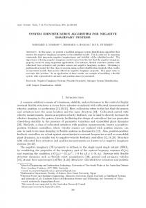
Figure 1 shows a two-compartment system which can have either real distinct or real repeated eigenvalues. Therefore, three possible mathematical models can be used to describe the system, (i) Model I : A,(e'" -e'") , 2nd order model with distinct
Z=[CIDIG]
and
in which
eigenvalues, (ii) Model 2: A , t e h " , 2nd order model with a pair of repeated eigenvalues, and (iii) Model 3: A,e'" +A,te"" , 2nd order model with a pair of repeated eigenvalues (general expression).
D=
koi
I
I
Figure I
G=
and 0cLLSrepresents the estimated 0 in the generalized linear least squares senses with initial
A(s)
provided by equation (9). Theoretically,
equation (25) is used iteratively until A(s) +A(s). However, i n practical applications, one or two iterations are sufficient to obtain satisfactory parameter estimates [5]. A case study to evaluate the GLLS algorithm for the identification of a nonuniformly sampled biomedical system with a pair of repeated eigenvalues is presented in the next section.
111. CASESTUDY The GLLS algorithm with distinct eigenvalues has been successfully applied in non-uniformly sampled biomedical system parameter estimation and
km
The two compatment model with input jn compa~tme~it I and output in compartment 2 respectively.
Suppose kzl = kO2= 1, k12 = kol = 0 and u(t) = 106(t), an impulse of magnitude 10, the impulse response of the system is y(t) = lOte-', which has a pair of repeated eigenvalues hl=h2=-1. In other words, Model 2 is the right model for the system. For the noise free data generated by y(t) = lOte-', we can easily use the GLLS algorithm to validate that Model 2 is the right model. To generate the noisy data, we added zero-mean white Gaussian noise with 5% coefficients of variation (CV) to y(t)> the model output. Model 1, Model 2 and Model 3 were then used to fit the noisy data using the GLLS algorithm respectively. The simulation study was performed using the PV-WAVE package. Numerous statistical tests can be used to compare the results of parameters estimation for determining the best fit model. In this paper, we use the analysis of weighted residuals sum of squares (WRSS), parameters estimate asymptotic coefficients of variation (CVs), the parameter correlation matrix (R), Akaike Information Criterion (AIC) [ l ] and Schwarz Criterion (SC) [8] to determine which model is the best. The results of the parameter estimation are summarized in Table 1. As seen in Table 1, the
562
Authorized licensed use limited to: Hong Kong Polytechnic University. Downloaded on June 25,2010 at 04:06:09 UTC from IEEE Xplore. Restrictions apply.
weighted residual sum of squares (WKSS) of the three models are very close, other criteria should be used to determine the best fit model. Compare Model 1 with Model 2, although the WRSS of Model 1 is smaller than that of Model 2, the parameter estimates in Model 1 have the largest asymptotic CVs whereas the asymptotic CVs of the parameters in Model 2 are much smaller. Moreover, the AICs and SCs of Model 1 are larger than those of Model 2, which are also in favour to Model 2. Furthermore, the parameter estimates in Model 1 are strongly correlated as shown in the correlation matrix R M M1,~whereas ~ ~ , the correlation matrix of Model 2, Rl\ldel 2, shows that the parameter estimates in Model 2 are less correlated. hl RModel1
=
1 2
-0.9869 0.9897 1.0000 -0.9615 -0.9615 1.0000 AI
1
AI
Based on the above arguments, it can be seen that Model 2 is better than Model 1 and we can reject Model 1 from our analysis. Now, we compare Model 2 with Model 3. Both models contain repeated eigenvalues and Model 3 being the general expression. The correlation matrix of Model 3 is given by h1 R ~ o d e 1 3=
A2
0.1183 -0.1830 1.0000 -0.6563 -0.6563 1.0000
From Table 1, it can be seen that the WRSS of Model 2 is less than that of Model 3. Moreover, comparison of the sub-matrix of R M ~3 ~ (the I resultant matrix of RModel after removing the first
row and the first column of &del 3) and the correlation matrix of Model 2 ( R ~ ~ o 2) d ~also l shows that Model 2 is better than Model 3 since the parameters in Model 2 are less correlated than those of Model 3. In addition, one of the parameters (A,) in Model 3 has a very large asymptotic CV (1 1.10%) and the asymptotic CVs of the other two parameters (A2 and AI) are slightly larger than those corresponding to the parameters A1 and AI in Model 2. The above comparisons suggest that Model 3 is not as suitable as Model 2 to describe the system. To further support of our arguments, we can consider the AICs and SCs of both models. As shown in Table 1, the AICs and SCs of Model 2 are smaller than those of Model 3, which in turn implied that Model 3 is over-parameterized to describe the system. In other words, Model 2 is better than Model 3 . Comparisons of the two rejected models (Model 1 and Model 3) also suggest Model 3 is still better than Model 1 since the correlation coefficients and the asymptotic CVs of the parameters i n Model 3 are much smaller than those of Model 1. Based on the above comparative arguments, we conclude that the best model to describe the system is Model 2 which is the exact form of the impulse response of the system that generated the data.
IV. CONCLUSION In this paper, a fast algorithm is presented, which can estimate continuous-time model parameters directly without the need of providing initial parameter values. Moreover, the algorithm can produce unbiased parameter estimates and it requires very little computing time. The case study presented demonstrates the reliability of the algorithm. With this algorithm, we can provide more choices for system identification and can find the best suitable model for the system from the non-uniformly sampled noisy data.
"Degree of Freedom = number of data point(N) - number of parameters(P) + number of conbtraintb 'VVaiiance Rdtin = WRSS/dP
563
Authorized licensed use limited to: Hong Kong Polytechnic University. Downloaded on June 25,2010 at 04:06:09 UTC from IEEE Xplore. Restrictions apply.
Unbiased Parametric Imaging Algorithm for Non-Uniformly Sampled Biomedical System Parameter Estimation”, ZEEE Trans. Med. Imag., accepted, 211996. 161 Hsia T.C., “System Identification: Least Squares”, Lexington Books, D. C. Heath and Company, 1977. [7] Mori F. and DiStefano J.J., 111, “Optimal Nonuniform Sampling Interval and Test Input Design for Identification of Physiological Systems from Very Limited Data”, IEEE Trans. Automatic Control, vol. 24, pp. 893-899, 1979. [8J Schwarz G., “Estimation of the dimension of a model”, Ann. Stat., VOI. 6, pp.461-464, 1978. [SI Wong K.P., Feng D., and Siu W-.C9 “Generalized Linear Least Squares Algorithm for Non-uniformly Sampled Biomedical System Identification With Possible Repeated Eigenvalues ”, Submitted to International Journal of Systems Science, 511996. [10]Yamamoto Y.L., Thompson C.J., Meyer E.E., Robertson J.S., and Feindel W., “Dynamic Positron Emission Tomography for study of Cerebral Hemodynamics in a Cross Sectjon of Head Using Positron Emitting 6*Ga-EDTA and 77Kr”, J . Comput. Assist Tomogr., vol.1, pp.4356, 1977.
ACKNOWLEDGEMENT We would like to acknowledge the support from the Australian Research Council (ARC) and the Research Committee of the Hong Kong Polytechnic University.
REFERENCES [ l ] Akaike H., “A Bayesian analysis of the minimum AIC procedure”, Ann. Inst. Stat. Math., vol. 30, pp. 9-14, 1978. [2] Astrijm K.J., “Maximum-likelihood and prediction error methods”, Automatica, vol. 16, pp.551-557, 1980. [3] Fagarasan J.T. and DiStefano J.J. 111, “Hidden pools, hidden modes and visible repeated eigenvalues in compartmental models”, Math. Biosci., vol. 82, pp.87-113, 1986. [4] Feng D., Ho D., Chen K., Wu L., Wang J., Liu R., and Yeh S., “An Evaluation of the Algorithms for Determining Local Cerebral Metabolic Rates of Glucose Using Positron Emission Tomography Dynamic Data”, IEEE Trans. Med. Zmag., vol. 14, No. 4, pp. 697-710, 1995. [ 5 ] Feng D., Huang S.C., Wang Z., and Ho D., “An
564
Authorized licensed use limited to: Hong Kong Polytechnic University. Downloaded on June 25,2010 at 04:06:09 UTC from IEEE Xplore. Restrictions apply.