Fast Transmit Antenna Selection Algorithms for MIMO Systems with Fading Correlation Hongyuan Zhang
Huaiyu Dai
Dept. Electrical and Computer Engineering North Carolina University Raleigh, NC USA
[email protected]
Dept. Electrical and Computer Engineering North Carolina University Raleigh, NC USA
[email protected]
Abstract—Motivated by some properties of the determinant
of Hermitian positive definite matrices, this paper develops some fast transmit antenna selection algorithms for MIMO systems based on instantaneous channel information or channel statistics for a correlated fading channel. The performances of these algorithms are evaluated in terms of both the resulted system capacity and error rate. The novel G-circles method can achieve many advantages over other existing algorithms. Keywords – MIMO; antenna selection; fading correlation
I. INTRODUCTION Multiple-input multiple-output (MIMO) systems are anticipated to be widely employed to address the everincreasing capacity demands for wireless communication systems. A major drawback of MIMO systems comes from the increased hardware cost caused by multiple analog/RF frontends, which motivated the investigation of antenna selection schemes [3][4][9][10]. For capacity maximization, the optimal selection comes from the exhaustive search over all possible antenna subsets [3][11]. On the other extreme, the simplest algorithm called power-based selection (PBS), selects the antennas with the largest channel gains and performs well only at low signal to noise ratio (SNR) regime [9][10]. Some other algorithms are proposed with good trade-offs between performance and complexity, for example, the novel near optimal iterative algorithms in [2][5], and the fast algorithm called correlationbases selection (CBS) in [1]. All the above algorithms require instantaneous channel state information (CSI), and are hard to be implemented for channel environments with fast fading or high mobility. On the other hand, in realistic outdoor channels, the channel correlation is a function of the local scattering environment and thus varies on a much slower time scale than instantaneous channel coefficients. There is little work in the literature done on antenna selection for capacity maximization based on channel statistic information. For error rate minimization in spatial multiplexing systems, we can find antenna selection algorithms based on both instantaneous CSI (e.g. [6]), and channel correlation matrices (e.g. [4][12]). An important figure of merit for error rate minimization is the maximization of the post-detect SNR in the weakest substream.
In this paper, motivated by the matrix determinant properties of Hermitian positive definite matrices, fast transmit antenna selection algorithms are explored considering both capacity and error rate, based on both instantaneous CSI and channel correlation matrix. Specifically, Gram-Schmidt algorithm performs near optimal, while the novel G-circles algorithm achieves many advantages over all the other existing schemes. II. SYSTEM MODEL AND PROBLEM FORMULATIONS Suppose there are N t transmit and N r receive antennas in a MIMO system. By using a block fading channel model, in each data block we select L transmit antennas out of the N t candidates and connect them to the available L RF chains. No CSI is available at the transmitter, so the selection is implemented at the receiver, and the selected antenna subset will be fed back to the transmitter so that the transmitter can equally allocate its power among L selected antennas. We denote H as the original N r × N t channel matrix, and H sl as the selected N r × L channel matrix. The spectral efficiency after antenna selection can be expressed as: ρ (1) C = log 2 det(I + H Hsl H sl ) , L where I is an L × L identity matrix, ρ is the transmit SNR. If only the transmitter side is under fading correlation, the corresponding channel matrix can be modeled as [7]: (2) H = H w (R1/t 2 ) H , H where R t = E H H is the N t × N t transmitter correlation matrix, and H w is an N r × N t normalized white Gaussian matrix. Note that in (2), H w models the fast Rayleigh fading, while R t represents the geometrical structure of the propagation channel and can be assumed to be unchanged over a much longer time-scale. The fading correlations can be expressed as: S
[ R t ]ik = β ∑ exp(2πj (i − k )( s =1
∆t
λ
) cos θ s ) ,
(3)
where β is a real positive scalar, ∆t is antenna spacing, λ is the wavelength, S is the number of major far-field scatterers at the transmitter side, and θ s represents the direction of departure (DOD) for the sth far-field scatterer. Suppose that S >> rank ( H ) , and ∆t is chosen to be large enough compared
with λ , the key factor influencing the channel conditioning is the range of DOD, or the angle spread of transmit scatterers. Maximizing (1) is equivalent to maximizing det( L / ρ I + H Hsl H sl ) . We can build a composite matrix: H , (4) G= L / ρ I N × N t t and let G sl be the corresponding sub-matrix after transmit antenna selection, whose first N r rows form the N r × L channel matrix H sl . By further defining (5) Z sl = G slH G sl , we can easily get that optimal selection is actually the exhaustive search for L columns in G that maximize det(Z sl ) . Assuming that L ≤ rank (H ) , then Z sl must be a Hermitian positive definite square matrix, which contains real positive eigen-values [8]. Also det(Z sl ) has the following important properties: • Property II.1: det(Z sl ) = (Π Rll )2 , where {Rll } are l
•
diagonal values of the upper triangular matrix R in the QR decomposition of G sl . Property II.2: det( Z sl ) = Πl λZ _ l , where {λZ _ l } are the
eigen-values of Z sl . In fast fading channels, transmit antenna selection algorithms based on instantaneous CSI is hard to be implemented in a real-time manner. Also, the antenna selection algorithms require the knowledge of the complete N r × N t channel matrix H, which requires the multiplexing of N t antennas to L RF chains during the training period. This will induce increased system overhead and possible erroneous channel estimations. Therefore it is desirable to develop antenna selection algorithms based on slowly varying channel statistics. At high SNR, we can approximate (1) by the equation det( L / ρ I + H slH H sl ) ≈ det( H slH H sl ) . If only fading correlation information is available for antenna selection, we need to maximize det( H Hsl H sl ) based on the knowledge of R t in (2). The channel matrix after transmit antenna selection is H sl = H w (R1/t _2sl ) H , in which R t _ sl is a certain principle minor of R t corresponding to the selected transmit antennas. From basic matrix determinant properties, we can get the following expression: det(H Hsl H sl ) = det(R1/t _2sl H wH H w (R1/t _2sl ) H ) . (6) = det((R1/t _2sl ) H R1/t _2sl H wH H w ) = det(R t _ sl ) det(H wH H w ) Since we cannot control the fast fading term det(H wH H w ) in (6), it is natural to get the following fact:
Fact II.1: To maximize (6) if only R t is available, L transmit antennas are chosen such that det( R t _ sl ) is maximized. In the following parts of this paper, fast antenna selection algorithms will be explored based on Properties II.1~2.
III. GRAM-SCHMIDT (GS) BASED ALGORITHM From Property II.1, to maximize the capacity, L transmit antennas with maximum Π Rll are selected. The GS method is l
suboptimal with greatly reduced complexity, which was first discussed in [2]. In each step, one antenna with the largest Rll is selected. The QR decomposition G sl = QR , is actually the complete ‘road map’ of the Gram-Schmidt process, in which R is an L × L upper triangular matrix, whose lth diagonal value Rll is a real positive number representing the ‘projection height’ of the projection from lth column vector g l , to the space spanned by g 1 ~ g l −1 . We can further explain the GS algorithm from a geometric standpoint, based on the following observation:
Observation III.1: The optimal transmit antenna selection for capacity maximization is equivalent to selecting L antennas such that the volume of the L-dimensional parallelotope generated by the L selected column vectors in G sl is maximized. From Property II.1 and the analysis of Rll above, we can easily get that such volume equals to Π Rll . See Figure 1 for l
two and three dimensional examples.
Figure. 1 Two and three dimensional examples of Gram-Schmidt process
In step l of the GS method, we select one antenna whose corresponding channel column vector has the largest ‘projection height’ to the space spanned by the previously selected column vectors, so that the volume of l-dimensional parallelotope can be maximized. Also note that a large ‘projection height’ in step l generally requires selecting g l with both a large norm and small correlations with g 1 ~ g l −1 , which results in a relatively well-conditioned H sl with large channel power, so that the capacity in (1) can be maximized. Since a V-BLAST detector takes QR decomposition of the (ordered) selected channel matrix H sl before the successive interference cancellation procedure [12][13], the GS method is also a good choice for the error rate minimization in a VBLAST system, because in general the smallest Rll , which represents the weakest data link, can be approximately maximized. This algorithm is fast because only vector/scalar multiplications and additions are involved. However, it requires instantaneous CSI and cannot be implemented only based on R t .
IV. GERSCHGORIN CIRCLES (G-CIRCLES) BASED ALGORITHM From Property II.2, to maximize the capacity, L transmit antennas with the largest Π λZ _ l are selected. Denoting {λl } as
antenna (l) has low correlations with all the other selected antennas.
l
the eigen-values of the square matrix T ( L ) = H Hsl H sl , it is easy to prove that λZ _ l = λl + L / ρ . Therefore, to maximize the capacity, we select H sl with L eigen-values as large as possible. A near optimal method is the exhaustive search to maximize the minimum eigen-value λmin (H slH H sl ) . Denoting T( l ) = (H ( l ) ) H H ( l ) , in which H( l ) = [h (1) , h(2) ," , h( l ) ] with (l ) as the selected antenna index in step l, and H sl = H ( L ) . Let λ1(l −1) ≥ λ2(l −1) ≥ " ≥ λl(−l1−1) be the eigen-values of T ( l −1) , while
T( l ) has eigen-values λ1(l ) ≥ λ2(l ) ≥ " ≥ λl(l ) . It is proved in [8] that:
λ
(l ) 1
( l −1) 1
≥λ
≥λ
(l ) 2
( l −1) 2
≥λ
( l −1) l −1
"≥λ
≥λ .
Therefore λmax ( H H sl ) is upper bounded by λmax (H H ) and a large λmin (H slH H sl ) results in a small channel conditioning
Theorem IV.1(G-circles): The L eigen-values of T ( L ) = H Hsl H sl are trapped in the circles centered at [T( L ) ]ll with radii given by the following expression:
λl − [T ]ll ≤ rl = min(∑ [T ]lk , ∑ [T ]kl ) . ( L)
( L)
(L)
k ≠l
Since T
is Hermitian, we get
(8)
k ≠l
∑ [T k ≠l
(L)
]lk = ∑ [T ]kl . From (L)
k ≠l
the definition of T( L ) , we can further simplify (8) by:
λl − h(l )
λmin ≥ min ( h (l ) 2 − ∑ h (Hk ) h ( l ) ) , 2
l =1,", L
H
number: κ = λmax / λmin , which is important for capacity maximization especially at high SNR. The maximization of λmin (H slH H sl ) is also a good antenna selection method for the BER minimization problem in spatial multiplexing systems with V-BLAST, or other linear receivers [6][12]. However, it requires the calculation of eigen-values for all antenna subset candidates. To simplify the selection algorithm, we will focus on the approximation of λmin (H slH H sl ) . It can be proved by (7) that λmin is decreased after each selection. Our strategy is: in each step we select one column in H so that the decrease of λmin can be approximately minimized. The G-circles theorem gives us an approximation of the distributions of eigen-values of T( L ) [8]:
( L)
A lower bound of λmin can be found from (9):
(7)
(l ) l
H sl
Figure. 2 An example of G-circles
2 2
≤ rl = ∑ h(Hk )h(l ) .
(9)
k ≠l
An example of G-circles for T(3) can be found in Figure 2. For T( L ) , all the L G-circles have positive centers. Since eigen-values are all real positive numbers (because T( L ) is positive definite), they are actually distributed on the real axis within the range of G-circles (the bold lines in Figure 2). From (9), a large center of the lth G-circle represents a large channel gain of transmit antenna (l), while a small radius means that
(10)
k ≠l
which is the left most point among all the L G-circles (point A in Figure 2). As discussed above, to approximately minimize the decrease of λmin in each step, we maximize the lower bound of λmin in (10), which motivates the following algorithm: Algorithm IV.1 (G-circles): Select h (1) from
H with the largest Euclidian norm h(1)
2
Update Remaining Set and Selected Set For l=2:L For i ∈ Remaining Set
h ( l ) _ temp = h i
Γ = {Selected Set , h ( l ) _ temp } LBi = min( h ( k ) k∈Γ
2 2
− ∑ h (Hj )h ( k ) ) j ≠k
End Select h ( l ) = h i with the largest
LBi
Update Remaining Set and Selected Set End
Initially, we select the antenna with the largest channel gain, and the G-circle of T(1) is only one point on the real axis. In the following steps, selecting one more antenna results in adding one more G-circle and the expansion of the radii of existing G-circles. From a geometric viewpoint, intuitively the maximization of (10) requires selecting one antenna with large norm and small fading correlations with all the other selected antennas, which generally results in a large ‘projection height’ (see Figure 1 and Observation III.1), so Algorithm IV.1 can achieve a performance close to the GS based algorithm. Compared with GS method, G-circles based algorithm is slightly simpler, because only vector multiplication and scalar additions are involved. It is also simpler than CBS algorithm proposed in [1], which requires the calculations of the correlation between any two transmit antenna candidates. Gcircles method performs uniformly better than CBS especially
for well-conditioned channels, which can be observed from the numerical results in Section V. The G-circles method is also applicable when only R t is available for antenna selection. From Fact II.1 and the property det(R t _ sl ) = Π λR _ l , one method for capacity l
maximization is to maximize λmin ( R t _ sl ) by the exhaustive search over all the L × L principle minors of R t . To avoid such exhaustive search, we further simplify it by the G-circles of R t _ sl : Algorithm IV.2 (G-circles - R t ) :
a = [R t ]ii ∀i → identical diagonals in R t Select h (1) and
h (2) such that [R t ](1),(2) is the minimum
Do the same procedure as Algorithm IV. 1, to select antennas (3)~(L), H
using [ R t ]i , j instead of hi h j , and
a
instead of h (i )
2 2
Note that in step 1, since all the diagonals of R t are identical, we do not have the freedom to select the antenna with the largest channel gain. Therefore initially we simply select two antennas with the smallest correlation. V. NUMERICAL RESULTS We simulate a MIMO system with N r = 3 , Nt = 9 , and L = 3 . (2)~(3) are used for the correlated channel model. In (3), we assume that ∆ t = 5λ , S = 100 , and θ1 ~ θ S are uniformly distributed in the range ( −∆θ / 2, ∆θ / 2) . Therefore, the channel conditioning number largely depends on ∆θ . In the first simulation, capacities achieved by antenna selection algorithms based on instantaneous CSI are investigated. Two extreme conditions: ∆θ = 180o , and ∆ θ = 15 o , are simulated representing well- and ill- conditioned channels, respectively. From Figure 3, we found that the GS algorithm perform near optimal for any channel conditioning situation, while the G-circles method is near optimal for wellconditioned channels. For ill-conditioned channels, the Gcircles method preserve the spatial multiplexing gain (see the slope of the curve in Figure. 3 (b) ), and is about 1dB away from the optimal selection at high SNR, which is a reasonable performance loss compared with its achieved complexity reduction. The G-circles method yields uniformly better performances over CBS, especially for well-conditioned channels.
channels. The R t -based G-circles method even outperform its counterpart based on instantaneous CSI for channels with ∆θ < 20o . An intuitive explanation is that, for ill-conditioned channels, R t _ sl dominates the eigen-value distributions in H Hsl H sl , and maximizing the lower bound of λmin ( R t _ sl ) by its G-circles is more effective than directly maximizing the lower bound of λmin (H slH H sl ) in (10). For well-conditioned channels, the R t -based algorithms converge to a performance with marginal selection gain. Finally we investigate the bit error rates for the proposed antenna selection schemes with V-BLAST receivers. QPSK modulation is employed in each of the three selected transmit antennas so that the throughput is fixed to be 6 bits/s/Hz. Generally speaking, the error rate performances have trends similar to their capacity counterparts in Figures 3 and 4. From Figure 5, we can see that in well-conditioned channels, the Gcircles method greatly outperforms CBS. The GS method performs close to the exhaustive search for the largest λmin (H slH H sl ) for any channel conditioning situation. For ill-conditioned channels, the R t -based G-circles method performs close to the exhaustive search for the largest λmin (Rt _ sl ) and achieves considerable selection gain over the MIMO system without antenna selection. VI. CONCLUSIONS In this paper, motivated by some matrix determinant properties of Hermitian positive definite matrices, we develop fast MIMO transmit antenna selection algorithms considering both capacity and error rate. The GS method is shown to achieve near optimal performances for any channel conditioning situation. For the simpler G-circles method, compared with optimal selection it reduces the complexity significantly with reasonable performance loss; compared with the GS method, it is simpler and can be implemented only based on R t ; compared with CBS, it is simpler with uniformly better performances and can be implemented for R t -based selection.
In the second simulation, we investigate Rt -based antenna selection algorithms. The transmit SNR is fixed to be 20dB and the capacity curves are drawn with respect to ∆θ . Also, we simulate the selection scheme that makes the exhaustive search for maximum det( R t _ sl ) in (6), which in general represents the optimal R t -based antenna selection for capacity maximization (Fact II.1). From Figure 4, we see that all the R t -based algorithms perform near optimal for ill-conditioned
(a) A well-conditioned channel
(b) An ill-conditioned channel
(b) An ill-conditioned channel
Figure. 3 Capacity performances for well- and ill-conditioned channels
Figure. 5 BER performances for well- and ill-conditioned channels
REFERENCES [1]
[2]
[3]
[4]
[5] Figure. 4 Capacities of
R t -based selections w.r.t. different ∆θ
[6]
[7]
[8] [9]
[10]
[11]
[12]
(a) A well-conditioned channel
[13]
Y. S. Choi, A. F. Molisch, M. Z. Win, and J. H. Winters, “Fast algorithms for antenna selection in MIMO systems”, Proc. IEEE Vehicular Technology Conference, Fall 2003, Orlando, FL., Oct. 2003. M. Gharavi-Alkhansari, and A. B. Gershman, “Fast antenna subset selection in MIMO systems”, IEEE Trans. Signal Processing, vol. 52, no. 2, pp. 339-347, Feb. 2004. D. A. Gore, R. U. Nabar, and A. J. Paulraj, “Selecting an optimal set of transmit antennas for a low rank matrix channel”, Proc. Int. Conf. Acoust., Speech and Signal Processing, Istanbul, Turkey, June 2000. D. A. Gore, R. W. Health, Jr. and A. J. Paulraj, “Statistical antenna selection for spatial multiplexing systems,” Proc. 2002 IEEE International Conference on Communications, vol. 1, pp. 450 -454 , New York City, 28 April- 2, May, 2002. A. Gorokhov, “Antenna selection algorithms for MEA transmission systems”, Proc. Int. Conf. Acoust., Speech and Signal Processing, vol. 3, pp. 2857-2860, May 2002. R. W. Health, Jr., S. Sandhu, and A. J. Paulraj, “Antenna selection for spatial multiplexing systems with linear receivers”, IEEE Communications Letters, vol. 5, no. 4, pp. 142-144, April 2001. M. T. Ivrlac, W. Utschick, and J. A. Nossek, “Fading correlation in wireless MIMO communication systems”, IEEE Journal on Selected Areas in Communications, vol. 21, no. 5, pp. 819-828, June 2000. C. D. Meyer, “Matrix analysis and applied linear algebra”, SIAM, 2000. A. F. Molisch, “MIMO systems with antenna selection-an overview”, Proc. Radio and Wireless Conference, 2003. RAWCON ’03, pp 167-170, Aug. 2003. A. F. Molisch, M. Z. Win, and J. H. Winters, “Capacity of MIMO systems with antenna selection”, Proc. IEEE Int. Conf. on Commu., ICC ’01, vol. 2, pp. 570-574, June 2001. R. U. Nabar, D. A. Gore, and A. J. Paulraj, “Optimal selection and use of transmit antennas in wireless systems”, Proc. Int. Conf. on Telecommunications, Acapulco, Mexico, May, 2000. R. Narasimhan, “Spatial Multiplexing with transmit antenna and constellation selection for correlated MIMO fading channels”, IEEE Trans. Signal Processing, vol. 51, no. 11, pp. 2829-2838, Nov 2003. P.W. Wolniansky, G. J. Foschini, G. D. Golden, R. A. Valenzuela, “VBLAST: an architecture for realizing very high data rates over the richscattering wireless channel,” 1998 URSI International Symposium on Signals, Systems, and Electronics, pp. 295 – 300, 29 Sept.-2 Oct. 1998.