Boolean algebra which was developed by George Boole in. 1854, is an algebraic structure defined by a set of elements, B. (i.e. B is defined as a set with only ...
(IJACSA) International Journal of Advanced Computer Science and Applications, Vol. 6, No. 1, 2015
Fast Vertical Mining Using Boolean Algebra Hosny M. Ibrahim
M. H. Marghny
Noha M. A. Abdelaziz
Information Technology Department Faculty of Computer and Information, Assiut University Assiut, Egypt
Computer Science Department Faculty of Computer and Information, Assiut University Assiut, Egypt
Information System Department Faculty of Computer and Information, Assiut University Assiut, Egypt
Abstract—The vertical association rules mining algorithm is an efficient mining method, which makes use of support sets of frequent itemsets to calculate the support of candidate itemsets. It overcomes the disadvantage of scanning database many times like Apriori algorithm. In vertical mining, frequent itemsets can be represented as a set of bit vectors in memory, which enables for fast computation. The sizes of bit vectors for itemsets are the main space expense of the algorithm that restricts its expansibility. Therefore, in this paper, a proposed algorithm that compresses the bit vectors of frequent itemsets will be presented. The new bit vector schema presented here depends on Boolean algebra rules to compute the intersection of two compressed bit vectors without making any costly decompression operation. The experimental results show that the proposed algorithm, Vertical Boolean Mining (VBM) algorithm is better than both Apriori algorithm and the classical vertical association rule mining algorithm in the mining time and the memory usage. Keywords—association rule; bit vector; Boolean algebra; frequent itemset; vertical data format
I.
INTRODUCTION
Data mining is defined as “The non trivial extraction of implicit, previously unknown and potentially useful information from databases” [1]. Association rules mining is an active research topic in the data mining field, which is the key step in the knowledge discovery process [2, 3]. Mining frequent itemsets (FIs) is the most important task in mining association rules. Furthermore, frequent itemsets detection can be used in other data mining tasks like classification and clustering [4-6]. Therefore a lot of mining frequent itemsets algorithms has been proposed. None of these methods can outperform other methods for all types of datasets with every minimum support [7, 8]. The well-known (FIs) mining algorithms are based on either horizontal or vertical data structures. Some of the horizontal based algorithms are Apriori, AprioriTid and FP-growth. Apriori is a level-wise algorithm that adopts an iterative method to discover frequent itemsets, in which k frequent itemsets is created by joining k-1 frequent itemsets, and then remove itemsets that contain nonfrequent items. Non frequent items are detected by scanning the database once for each itemset to calculate its support. This is the most important shortcoming of Apriori algorithm [9]. AprioriTid has been proposed to improve Apriori algorithm‟s efficiency by reducing the overhead of I/O by scanning the database only once in the first iteration [9]. FP-growth algorithm mines frequent item sets by scanning the database only two times without candidate generation. It also compresses the data set into a data structure called FP-tree. FP-
growth finds all the frequent item sets by searching the FP-tree, recursively [10]. Eclat, BitTableFI and IndexBitTableFI are some examples of vertical based (FIs) mining methods. Eclat uses a structure called Tidset, which store the transaction identifiers for each itemset. The support of an itemset X can be fast derived as the cardinality of the Tidset of the itemset. Thus, the support(X) = |Tidset(X)|. It also proposed the way of computing Tidset(XY) by the intersection operator between Tidset(X) and Tidset(Y). That is, Tidset(XY) = Tidset(X) ∩ Tidset(Y) [11]. In BitTableFI [12] each item occupied |T| bits, called a bit vector, where |T| is the number of transactions in D. The bit vector of a new itemset XY from the two itemsets X and Y could be easily derived by the AND operation on the two bit vectors of X and Y. Because the length of the two bit vectors was the same, the result would be a bit vector with the same length of |T| bits. Dong and Han used the BitTable to mine frequent itemsets based on the level-wise concept in the Apriori algorithm [9]. Their approach was named BitTableFI [12]. Note that in the Apriori algorithm, the supports were computed by re-scanning databases, while in the BitTableFI approach, they were derived by the intersection of bit vectors. The support of an itemset could be found by counting the number of „1‟ bits in its corresponding bit vector. Later, in Song et al. [13], Index-BitTableFI employed index array to improve the algorithm. From the above discussion, the following points can be concluded: vertical association rule algorithms conquer some disadvantages of horizontal ones, vertical association rule algorithms need memory space too much when the dataset is too large. In order to overcome this issue, in this paper, a proposed algorithm that depends on a simple representation of frequent itemsets, which is, compressing the support sets bitmap of data itemsets that to be sent to memory, so as to save the space required by the algorithm. It contributes to reducing not only the execution time but also the required memory. The rest of this paper is organized as follows; Section II briefly revisits some association rule background information. The difference between vertical and horizontal data formats are listed in Section III. Boolean Algebra rules and theories are given in section IV. In Section V, the new algorithm, VBM algorithm is proposed. Section VI analyzes the performance of the proposed algorithm and conclusion is given in Section VII. II.
BASIC CONCEPTION
Association rule mining involves detecting items which tend to occur together in transactions and the association rules that relate them [14].
89 | P a g e www.ijacsa.thesai.org
(IJACSA) International Journal of Advanced Computer Science and Applications, Vol. 6, No. 1, 2015
Consider I= {i1, i2,………,im} as a set of items. Let D, the task relevant data, is a set of database transactions where each transaction T is a set of items such that T is a subset of I. Each transaction is associated with an identifier, called TID. Let A be a set of items. A transaction T is said to contain A if and only if A⊆T. An Association Rule is an implication of the form A⇒B, where A⊂I, B⊂I, and A∩B=φ. Rule support and confidence are two measures of rule interestingness. They respectively reflect the usefulness and certainty of discovered rules. The rule A⇒B holds in the transaction set D with support s, where s is the percentage of transactions in D that contain A∪B (i.e., the union of sets A and B, or say, both A and B). This is taken to be the probability, P(A∪B). That is,
Support (A⇒B) = P(A∪B).
determined by the first step, here we are concentrating only on the first step. III.
(1)
TABLE I.
The rule A⇒B has confidence c in the transaction set D, where c is the percentage of transactions in D containing A that also contain B. This is taken to be the conditional probability; P(B |A) .That is,
Confidence (A⇒B) = P(B|A)= =
Support(𝐴∪𝐵) Support(𝐴) Support_Count(𝐴∪𝐵) Support_Count(𝐴)
A minimum support threshold and a minimum confidence threshold can be set by users or domain experts. Rules that satisfy both a minimum support threshold (min_support) and minimum confidence threshold (min_confidence) are called strong. The objective of association rule mining is to find rules that satisfy both a minimum support threshold (min_support) and minimum confidence threshold (min_confidence) .Thus the problem of mining association rules can be reduced to that of mining frequent itemsets. In general, the problems of association rules can be divided into two sub ones [17, 18]: 1) Find out all the frequent itemsets in database D according to the minimum support. 2) Generate association rules from frequent itemsets with the limitations of minimal confidence. Since the second step is much less costly than the first and the overall performance of mining association rules is
A TRANSACTION DATABASE
TID 1
Item A, C, D
2
A, B, D, E
(2)
The definition of a frequent pattern relies on the following considerations. A set of items is referred to as an itemset (pattern). An itemset that contains K items is a K-itemset. The set {X, Y} is a 2-itemset. The occurrence frequency of an itemset is the number of transactions that contain the itemset. This is also known as the frequency or the support count of an itemset [15]. An itemset satisfies minimum support if the occurrence frequency of the itemset is greater than or equal to the minimal support threshold value defined by the user [16]. The number of transaction required for the itemset to satisfy minimum support is therefore referred to as the minimum support count. If an itemset satisfies minimum support, then it is a frequent itemset.
VERTICAL ASSOCIATION RULES MINING
Horizontal and vertical data formats are two common kinds of data formats to be adopted in frequent itemsets mining. Horizontal structure is the data distribute way by most association rules mining algorithm, its dataset is made up of a series of transactions, each of them includes transaction‟s ID TID and relevant transaction‟s inclusive itemsets. However, vertical structure is that the dataset is made of a series of items; each of the items has its TID-list that is the ID list including all transaction of this item [19]. Table I shows transaction database. Fig. 1 and 2 show respectively horizontal and vertical structures for database in Table 1.
1 2 3 4 5 6
3
B, C, E
4
A, B, C, D
5
C, D, E
6
A, B, C, D, E
A C D 1 A B D E 1 B C E A B C D 1 C D E A B C D E 1
Fig. 1. Horizontal structure
A
1
2
4
6
B
2
3
4
6
C
1
3
4
5
6
D
1
2
4
5
6
E
2
3
5
5
Fig. 2. Vertical structure
Algorithms for mining frequent itemsets based on the vertical data format are usually more efficient than those based on the horizontal, because the former often scan the database only once and compute the supports of item sets fast [20]. IV.
BOOLEAN ALGEBRA
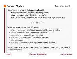
Boolean algebra which was developed by George Boole in 1854, is an algebraic structure defined by a set of elements, B (i.e. B is defined as a set with only two elements 0 and 1 in two
90 | P a g e www.ijacsa.thesai.org
(IJACSA) International Journal of Advanced Computer Science and Applications, Vol. 6, No. 1, 2015
valued Boolean algebra), together with two binary operators, (+) and (•), providing that the following postulates are satisfies[21]: Note:
Here is listed only the postulates which are of interest to that work not all Boolean algebra postulates.
In two valued Boolean algebra, zero and one define the elements of the set B, and variables such as x and y merely represent the elements.
The primary goal of the compression function is to make each vector starts and ends with consecutive zeros and then it gets rid of these zero bits to compress the vector. For each bit vector in the bitmap the compression function examines the start and the end of that vector. Three cases could be found: Case1: the vector starts and ends with sequence of zeros.
1. (a) The element 0 is an identity with respect to +; that is, x + 0 = 0 + x = x. 1. (b) The element 1 is an identity with respect to •; that is, x • 1 = 1 • x = x.
Case2: the vector starts and ends with sequence of ones.
2. (a) The structure is commutative with respect to +; that is, x + y = y + x. 2. (b) The structure is commutative with respect to •; that is, x • y = y • x. 3. For every element x ∈ B, there exists an element xʹ ∈ B (called the complement of x) such that (a) x + xʹ = 1 and (b) x • xʹ = 0. Duality principal of Boolean algebra states that: every algebraic expression deducible form the postulates of Boolean algebra remains valid if the operators and identity elements are interchanged, simply interchange OR and AND operators and replace 1‟s by 0‟s and vice versa as shown in parts a and b in the above postulates.
Case3 (a): the vector starts with sequence of ones and ends with zeros.
Case3 (b): the vector starts with sequence of zeros and ends with ones.
Some important theorems that were derived from the above postulates: 1: (a) x + x= x. (b) x • x= x. 2: (a) x + 1= 1.
Fig. 3. Example of transactions before and after compression
(b) x • 0= 0. 3: involution (xʹ) ʹ = x. 4: DeMorgan (a) (x + y) ʹ = xʹyʹ. (b) (x y) ʹ = xʹ + yʹ. V.
VERTICAL BOOLEAN MINING ALGORITHM (VBM)
This section divided into three subsections the first subsection V.A. describes the schema of bitmap used and its compression function. The intersection methods of the compressed vectors are described in V.B. Finally the detailed steps of the algorithm are illustrated in the last subsection V.C. A. Schema of bitmap used and its compression function This algorithm is based on vertical data format but instead of representing each item with a bit vector of fixed length equal to the total number of transactions, it uses compression function that works as described below.
In case 1, the compression function does not change the vector form. In case 2, the compression function sets the vector in its complement form to make it starts and ends with sequences of zeros as in case 1. In the third case the compression function counts the number of sequential zeros and the number of sequential ones in the front and tail of the vector. The compression function leaves the vector in its original form if the number of zeros counted is greater than number of ones and puts it in the complement form in the opposite case. For all three cases given in Fig. 3, the algorithm uses a new data structure for vectors. The vector consists of three elements. The first element, flag, Boolean value which indicates either the vector is in the original form (i.e. when flag=0) or complement form (i.e. when flag=1). The second element, removed (abbreviated as rem), binary value representing the number of zeros or ones removed from the beginning of the bit vector.
91 | P a g e www.ijacsa.thesai.org
(IJACSA) International Journal of Advanced Computer Science and Applications, Vol. 6, No. 1, 2015
The third element, data, list of bits representing the remaining bits after removing sequences of zero bits or one bits at the front and the tail of the old vector. B. How to intersect two compressed bit vectors and calculate their support Fundamental idea: In order to enhance algorithm‟s operation speed after compressing bitmap, the algorithm makes use of Boolean algebra's rules and postulates to intersect two compressed bit vectors and to calculate their support fast without making any decompression operation for itemsets‟ bit vectors. During intersecting two compressed bit vectors according to the schema illustrated above one of the following three cases will be occured: Case 1: the two vectors are in the original form (i.e. flag1=flag2=0). Initially, the decimal equivalents of the “rem” values of the two vectors are compared and the larger is used as the “rem” value of the resulting vector. Then AND operations are performed for the data parts of the two bit vectors. These operations start at position zero for the vector of larger “rem”. The starting point for the AND operation in the other vector is the difference between the decimal equivalents of vectors‟ “rem” values. If an initial resulting value is 0, then the “rem” value of the outcome vector is increased by 1 until the first non-zero resulting value is reached. Next, from the position of non-zero bit, all the resulting bits by the AND operation are kept in the outcome vector‟s data part except the last consecutive zero bits. Finally the resulting vector‟s flag value is set to zero indicating that the result of intersecting two original bit vectors is a vector in the original form. An example is given below to illustrate the intersection operation on case 1. Assume there are two vectors in the original form: {0, 11, {1, 1, 1, 0, 0, 1}} and {0, 111, {1, 1, 0, 1, 0, 1, 1, 1}} and their intersection is to be found. Both vectors are in the original form because their flags equals to 0. Because the “rem” value (111) of the second vector which is corresponding to 7 in decimal is larger than that (11) of the first that means 3 in decimal system, the AND operation then begins from position (7-3= 4) of first vector and position (0) of the second, at which the result of 0 and 1 is 0. The resulting “rem value” increased by one to be 8. Then, the result of next bits 1 AND 1 is 1 not equals to zero. The rest bits of the second vector are automatically removed because they haven‟t corresponding bits in the first vector which means that those bits in the first vector were zero bits so that the compression function removed them, and the results are all 0. The resulting vector is then {0, 1000, {1}}.The process is shown in Fig. 4. Case 2: one vector is in the original form and the other is in the complement form (i.e. flag1=0, flag2=1 or vice versa). The result of intersecting two vectors in different forms as in this case is a vector in the original form so the outcome vector‟s flag value is set to zero. The “rem” value of the resulting vector initially equals to that of the vector in the original form whether it is the larger or not. Then the decimal equivalents of the “rem” values of the two vectors are compared, if the “rem” value of the original vector is the
larger, the AND operations start at position zero for data part of the original vector and from position equals to the difference between original vector‟s “rem” and complement vector‟s “rem” for data part of the complement vector. If an initial resulting value is 0, then the “rem” value of the outcome vector is increased by 1 until the first non-zero resulting value is reached. But if the complement vector‟s “rem” is the lager, the first complement vector‟s “rem” value minus original vector‟s “rem” value bits of the original vector are added to the data part of the resulting vectors as they are, because those bits are corresponding to bits of value 1 that were removed from the complement vector in its original form and according to Boolean algebra postulates element 1 is an identity element with respect to AND operation. Next, AND operations are performed between the bits of the original vector and the complement of bits in the complement vector and the resulting bits are kept in the outcome vector‟s data part except the last continuous zero bits. An example is given below to illustrate the intersection operation on this case. Two vectors are given the first is in the original form: {0, 11, {1, 1, 1, 0, 0, 1}} and the second is in the complement form {1, 111, {1, 0, 0, 0, 0, 1, 1, 1}} as shown by their flags, and their intersection is to be found. Initially the “rem” value of the resulting vector will be 3 because the “rem” value of the original vector is (11) that means 3 in decimal system. Then the first 4 bits in the original vector will be put in the data part of the resulting vector, because those bits in the original vector were actually corresponding to 4 ones in the complement 1
1
1
0
0
1
& 1
1
0
1
0
1
1
1
1 Fig. 4. Intersection Example
vector before compression (i.e. 7-3=4 where 7 is the “rem” of complement vector greater than 3, “rem” value of original one). Next the AND operation starts at bit number 4 in the original vector and position (0) of the complement one, at which the result of 0 and 1 is 0. The resulting position then moves backward to 8. Then, the result of next bits 1 and 1 is 1 not equals to zero. The rest bits of the second vector are automatically removed because they haven‟t corresponding bits in the first vector which means that those bits in the first vector were zero bits so that the compression function removed them, and the results are all 0. The resulting vector is then {0, 11, {1,1,1,0,0,1}}.The process is shown in Fig. 5 and the opposite is given in Fig. 6 for vectors {0,11,{1,1,1,0,0,1,1,1}}and {1,10,{1,1,1,0,1,0,1}}with result equals{0,101,{1,0,0,0,1,1}}. Case 3: the two vectors are in the complement form (i.e. flag1=flag2=1). In this case the resulting vector of intersecting two vectors in the complement form is a vector in the complement form, but in some cases this complemented vector may require
92 | P a g e www.ijacsa.thesai.org
(IJACSA) International Journal of Advanced Computer Science and Applications, Vol. 6, No. 1, 2015
transforming to the original form according to some conditions that will be described in the algorithm in section V part c. Depending on Demorgan theory illustrated in section IV, the algorithm follows steps that are exactly the opposite to those that were followed in case 1. Case 3 intersection steps are illustrated here by an example shown in Fig. 7. 1
1
1
0
1
0 &
1
&! 1 !! 0
& 1
1
0
1
0
0
0
0
0
1
1
C. How VBM algorithm works The main steps of the algorithm can be summarized as follows.
1
First Step: Scan the database once, obtain a compressed bit vector for each data item by the aforementioned method and set up the result in the structure that were described in section V.A, and calculate support of each data item to produce frequent 1-itemsets and its related compressed bitmap.
1
Fig. 5. Intersection Example
0 &
1
1
1
0
0
1
1
&! 1
1
1
0
1
0
1
1
0
0
0
1
Hint: support of items represented by vectors in the original form is calculated by counting the number of set bits in the data part of that vector (i.e. number of “1” bits). But support of items represented by complemented vectors is
& 1
1
operations between each two corresponding bits till reaching the end of one of the bit vectors as shown in Fig. 7. 4) If the bits of one of the vectors finished before the other, the remaining bits of the longer vector will be placed as they are in the data part of the resulting vector, because those bits are actually corresponding to zeros of the shorter vector as discussed in step 2. 5) Finally the resulting vector is equals to {1,11,{1,1,1,0,1,1,0,1}}.
1
1
0
1
0
1
0
0
1
||
Fig. 6. Intersection Example
Note that: In Fig. 5 and 6 the algorithm automatically puts any bit above sign ( ) in the data part of the resulting bit vector and removes any bit below sign ( ) without actually making AND operation to those bits with 0 and 1, depending on Boolean algebra rules illustrated above in order to save execution time. Fig. 7 shows {1,11,{1,0,1,0,1,0,0,1}} and {1,100,{1,1,0,0,1,0,1}} two compressed bit vectors in the complement form assuming that the original length of the bit vectors before compression is 15 bit. The result is to be obtained by the following steps: 1) The “rem” value of the resulting vector equals to the smallest “rem” value of the two vectors As rem1=11< rem2=100 (i.e. 3 < 4 in decimal system), therefore the resulting “rem” value=3. 2) The (rem2-rem1) first bits of the vector with the smallest “rem” value are placed as they are in the data part of the resulting vector according to postulate 1(a) in section IV , because those bits are actually corresponding to zeros in rem2. As rem2-rem1= 4-3= 1 bit therefore first bit only of the first vector is to be put in the first bit of the data part of the resulting vector as shown in Fig. 7. 3) Since the intersection operation of two original vectors is accomplished through AND operations, therefore the opposite is done here according to Demorgan theory (i.e. (x•y)ʹ=xʹ+yʹ) aforementioned in section IV, using An OR
1
1
1
0
0
1
0
1
1
1
0
1
1
0
1
Fig. 7. Intersection Example
equals to the total number of transactions minus the number of set bits in the data part of the bit vector. Second step: In order to get the higher order candidate and frequent (k+1)-itemsets Fk+1 for each k>1, given a frequent kitemset Fk, the algorithm uses Depth-first method to join each two itemsets if they have the same first k-1 items (excluding just the last item) and the last item of first k-itemset comes before the last item of the second k-itemset in Fk, and applies a modification of the intersection function, which works on three components of the bit vector consisting of the flag part, removed value and the data part, so that obtaining higher order frequent (k+1)-itemsets does not require rescanning the database again. Third step: the intersection function first checks flags of both bit vectors to be intersected to detect which type of intersection needs to be followed as illustrated in section V.B, in section V.B. cases 1 and 2 are straightforward but case 3 may return vector either in the original or complement form. Case 3 returns vector in the complement form if the rem values of both vectors aren‟t equal to zero and the total of the length of the data part of the bit vectors plus the decimal equivalents of their rem values (i.e. number of removed zeros) is less than the total number of transactions, because this means that both original vectors were starting and ending with ones so the
93 | P a g e www.ijacsa.thesai.org
(IJACSA) International Journal of Advanced Computer Science and Applications, Vol. 6, No. 1, 2015
result will for sure starts and ends with ones, so the resulting vector should be returned as it is (i.e. in the complement form). Case 3 returns vector in the original form (i.e. case 3 will return the complement of the complemented vector section IV Theorem3 involution) if one of the previous conditions aren‟t satisfied. Examples on case 3: a) intersection method returns complement vector: the result of intersecting {1,11,{1,0,1,0,1,0,0,1}} and {1,100,{1,1,0,0,1,0,1}} equals {1,11,{1,1,1,0,1,1,0,1}}. b) intersection method returns original vector: the result of intersecting {1,0,{1,1,1,0,1,1,1}} and {1,101,{1,1,0,0,1,0,1,1,1,1}} equals {0,11,{1,0,0,0,1,1,0,1}}. Forth step: after detecting which type of intersection needs to be followed, the intersection operation is accomplished as illustrated in details in section V.B. to obtain the resulting bit vector. Then support count is calculated for the result. If support count>= min_support the result is added to frequent k+1 itemset or removed otherwise. Finally, this process will be continued until there aren‟t any longer frequent (k+1)-itemsets, then the algorithm ends. The proposed VBM approach and the schema of bit vectors used consume less time for computing the intersection among compressed bit vectors and for counting the number of 1 bits in the resulting bit vector due to their shorter lengths so the number of bits to be checked is smaller than in the case of classical vertical association rule mining algorithms.
vertical association rules algorithm without compressed bitmap, along with different minimum supports. It could be observed that the VBM algorithm was always faster than the other two in all the results. Next, experiments were conducted to compare between the VBM total memory usage (in MBs) and the vertical association rules algorithm without compressed bitmap. The VBM algorithm compression percentage is also calculated. The results for the three databases under different min_support values are shown in Table III. From Fig. 8 to 10 we can see that the mining time of VBM algorithm is far from Apriori algorithm but not faraway from the mining time of vertical association rules algorithm without compressed bitmap. But VBM decreased much in memory used by frequent itemsets bitmap than vertical association rules algorithm without compressed bitmap as illustrated in Table III. Regarding execution time, the non-parametric wilcoxon significance test has been performed to proof the efficiency of the VBM algorithm for the three datasets. The results of the test are given in Table IV. The VBM algorithm showed significant results when compared to Apriori algorithm and the vertical association rules algorithm as p-value