In this paper we propose a novel super-resolution algorithm based on motion compensation and edge-directed spatial interpolation succeeded by fusion via ...
FAST VIDEO SUPER-RESOLUTION VIA CLASSIFICATION K. Simonyan, S. Grishin, {simonyan, sgrishin}@graphics.cs.msu.ru
D. Vatolin, Member, IEEE, and D. Popov {dmitriy, dpopov}@yuvsoft.com
Moscow State University, Graphics & Media Lab
YUVsoft Corp.
ABSTRACT
backward projection algorithm [4] by making it more robust to optical flow estimation errors and by modeling the PSF via an elliptical weighted area filter. Freeman et al. [5] proposed an example-based image magnification method. Ⱥ large database storing the relationship between mediumand high-frequency patches was used to add plausible highfrequency information to the enlarged image. This technique combined with the reconstruction constraint was used by Wang et al. [6] for SR. The method, however, exhibits enormous computational complexity. Li [7] investigated the special case of SR given a set of LR frames acquired at different focal lengths. Static SR methods, if directly applied to each video sequence frame, can not provide the temporal consistency of the enlarged video, which impedes their application for video resolution enhancement. The problem of producing HR video from LR video (dynamic SR) has also been addressed. Bishop et al. [8] extended the approach of [5] to video resolution enhancement; special priors were introduced to maintain the temporal consistency of the enlarged video. As any example-based method, it is quite dependent on the training set. Cheung et al. [9] applied epitomic analysis to video resolution enhancement. This technique, however, is suitable only for processing video containing scenes obtained at different focal lengths. Farsiu et al. [1] used the Kalman filter approximation to bind the frame being enlarged with the previously processed frame. A translational motion model was assumed. Modern SR algorithms, therefore, exhibit two main shortcomings: huge computational complexity and the necessity of a priori knowledge about camera characteristics and motion models. These shortcomings restrict the algorithms’ field of practical application mainly to cases where a sequence of LR images, acquired from spatially close points or with varying focal length, is to be processed. These algorithms are unsuitable for real-time or near-realtime resolution enhancement of video streams. In this paper we propose a SR algorithm based on HR images fusion via pixel classification. The low computational complexity of the proposed method makes it suitable for fast video processing. Performance superiority over standard video upscaling methods is shown. The rest of the paper is organized as follows. In Section 2 our SR method is described. Experimental results are presented in
In this paper we propose a novel super-resolution algorithm based on motion compensation and edge-directed spatial interpolation succeeded by fusion via pixel classification. Two high-resolution images are constructed, the first by means of motion compensation and the second by means of edge-directed interpolation. The AdaBoost classifier is then used to fuse these images into an high-resolution frame. Experimental results show that the proposed method surpasses well-known resolution enhancement methods while maintaining moderate computational complexity. Index Terms — super-resolution, dynamic superresolution, video resolution enhancement, pixel classification, edge-directed interpolation, AdaBoost. 1. INTRODUCTION The problem of video resolution enhancement is currently of great importance due to the emergence of high definition (HD) displays. Since most video content is still lower resolution, special algorithms are needed to convert video to higher resolution. Algorithms for video resolution enhancement can be divided into two groups according to the type of information used. The first group is composed of algorithms that use the information only from the current video frame. Methods from this group (e.g. bilinear and bicubic interpolation) are widely used due to their low computational complexity. The second group consists of the so-called super-resolution (SR) algorithms. In this case the information from neighboring frames is also used, which leads to higher enlargement quality at the cost of higher computational complexity. Most contemporary SR algorithms are aimed at producing one high-resolution (HR) frame from a set of low-resolution (LR) frames. According to [1], we call them static SR algorithms. Various approaches have been taken recently in this field. Farsiu et al. [2] examined the LR image acquisition process in whole. They treated SR as an energy minimization problem and used robust regularization based on bilateral total variation to construct an HR frame. This method assumes affine motion in the sequence and considers the point spread function (PSF) of the camera to be known. Jiang et al. [3] improved the classical iterative
978-1-4244-1764-3/08/$25.00 ©2008 IEEE
349
ICIP 2008
Section 3. Section 4 concludes the paper and points some directions of future research.
~ H n �1
2. PROPOSED SUPER-RESOLUTION ALGORITHM
Ln I. Motion compensation
2.1. Algorithm Outline We consider the case of two-times magnification of spatial resolution; the other cases can be easily reduced to this one. It is also assumed that a pixel of LR frame is the mean of four corresponding pixels of this frame in high resolution. Our approach can be considered as an extension of that described in [1]. An unknown HR frame H n (the upper index represents the frame number) is modeled by an output ~ frame H n , which is constructed in three steps: 1. Motion compensation. The current LR frame Ln is compensated from already constructed previous HR ~ frame H n �1 to form an HR image M (Section 2.2). n
2. Spatial interpolation. L is upscaled using EdgeDirected Interpolation (EDI, Section 2.3) to form an HR image U . ~ 3. Fusion. The resultant frame H n is constructed via pixel-wise fusion of two HR images, M and U . Pixel fusion coefficients are calculated via the AdaBoost [10] classifier (Section 2.4). The flowchart of the algorithm is presented in Fig. 1.
Block-based motion estimation (ME) with adaptive block size (16×16 and 8×8) is used, as it’s fast and capable of capturing complex motion in a video sequence. Motion vectors are found with quarter-pixel accuracy. The ME algorithm takes the variance of blocks luminance into account, producing smooth motion vector fields in uniform areas. ME is performed in luminance plane only. The architecture of SR ME differs from that of conventional ME, as the resolution of the current frame is two times smaller in each direction than the resolution of the reference frame. The same is true for the current block and its corresponding reference block. But under the assumption of dependency between LR pixel (pixel of LR frame) and corresponding HR pixels (pixels of HR frame) the adaptation of motion compensation to SR is straightforward. The following metric function U is used to compare an LR block B with an HR reference block pointed by a motion o
vector d :
¦
� x, y B
o· ~§ Ln �x, y � L ¨¨ x, y, d ¸¸ , ¹ ©
III. Fusion
U
~ Hn Fig. 1. Flowchart of the proposed algorithm. where o· ~§ L ¨¨ x, y, d ¸¸ © ¹
o o 1 1 ~ n �1 § ¦ H ¨¨ 2 x � d x � i, 2 y � d y � 4 i, j 0 ©
· j ¸¸ ¹
(2)
is the pixel of a reference block converted to low resolution using bilinear downsampling. Thus, the metric is an adaptation of the Sum of Absolute Differences (SAD) metric to the SR framework. After a motion vector is estimated for each block, the HR motion-compensated frame M is built from the HR reference blocks. 2.3. Spatial Edge-Directed Interpolation Lattices of LR and HR pixels are illustrated on Fig. 2; LR pixels are shown as circles, HR pixels – as squares. For LR pixel i the set of corresponding HR pixels is
2.2. Motion Compensation
§ o· ȡ¨¨ B, d ¸¸ ¹ ©
M
II. Spatial interpolation
(1)
350
Ȇ�i
^ jk (i)`4k
1.
Consider an area ȍ formed by LR pixels
i, k , l , m with intensities A, B, C, D. At first, the luminance variance of ȍ is calculated. If it is less than a certain threshold T1 , the area is considered uniform, and bilinear interpolation is used for HR pixels belonging to ȍ . Otherwise, two possible cases are considered: an edge passes through ȍ , or ȍ contains texture. To determine the right case the following values are compared:
B � C , d2 � A � C � B � D / 2, h d1
v
x
A� D,
� A � B � C � D / 2 .
(3)
If d 2 ! d1 � T2 , where T2 is a threshold, the edge passes through LR pixels B and C (this case is depicted on Fig. 2). Pixels F and G are interpolated from B and C using linear interpolation. To obtain HR pixel H value, an imaginary line is drawn parallel to the edge through the pixel (dashed line in Fig. 2). Let H1 and H2 be the luminance values at intersections of the line with LR lattice. H1 is linearly interpolated from C and D; H2 is interpolated from B and D. And finally, H is linearly interpolated from H1 and H2. Pixel E is processed in the same way.
j1 �i
j2 �i
following sums of squared errors were calculated:
i
ȍ
m
l
Fig. 2. Correspondence between LR and HR pixels. x x
x
Else if d1 ! d 2 � T2 the edge passes through LR pixels A and D, and the interpolation is performed similarly. Else if v � h ! T2 the horizontal or vertical edge is present, and the aforementioned interpolation technique is applied. Else there is no dominant edge direction, and ȍ is considered belonging to the textured area. In this case Lanczos filter of radius 4 (lanc4) is used to obtain HR pixels’ values.
2.4. Images Fusion via Classification
After M and U HR images are built, a per-pixel fusion process is performed to construct an output HR frame. We introduce a probabilistic framework for the fusion process, modeling an unknown HR pixel value
H nj
(the lower index
represents the pixel number) by a random variate Hˆ nj for which two possible cases are considered:
^
Hˆ nj Mˆ j
ˆ M j � ǻM i j ,U j
`
U j � ǻUi ,
j Ȇ�i , i 1,..., Ln .
(4)
according to the upscaling errors 'M and 'U , which are defined as Lni � mean M j , ǻUi jȆ �i
Lni � mean U j . j Ȇ �i
2
jȆ �t
�
ˆ
2
¦ H nj � Uˆ j .
jȆ �t
(6)
approximated by substituting Lni instead of H nj for each j from 3 �i : ˆ
ˆ
SSE M � SSE U |
(5)
It is assumed that, for each LR pixel i , all four pixels from P�i are simultaneously taken either from Mˆ or from Uˆ . Thus, the AdaBoost classifier can be employed to estimate the class ci for each LR pixel i , where ci 1 if pixels from P�i are taken from Mˆ , and c �1 otherwise.
�
�
j Ȇ �i
¦ �Mˆ j � Uˆ j Mˆ j � Uˆ j � 2 H nj |
jȆ �i
¦ �Mˆ j � Uˆ j Mˆ j � Uˆ j � 2 Lni
X5 .
(7)
Three boosting iterations were performed to train a classifier. A small number of weak learners in the committee ensured the low computational complexity of the classifier. From our experiments, better results can be achieved, if n H is modeled by the expectation of Hˆ n , i.e., by j
~ H nj
j
Ǽ Hˆ nj
pi Mˆ j � �1 � pi Uˆ j , j Ȇ�i , i 1,..., Ln .
(8)
Here, pi P�ci 1 | X is the class conditional probability, which, according to [10], can be written as pi
Mˆ j and Uˆ j are the pixels of M and U , corrected
ǻM i
¦ H nj � Mˆ j , SSE U
The class that corresponds to the lower sum was chosen. A Classification And Regression Tree (CART) of depth 5 was used as a weak learner. The feature vector X consists of five features. The first two are the upscaling errors (5). The third is the luminance variance of neighboring LR pixels. The fourth is the sum of variances of the motion vector coordinates, calculated for neighboring blocks. The fifth feature is derived as follows: the difference between the sums of squared errors (6) is
j4 �i
j3 �i
�
ˆ
SSE M
k
1 / �1 � exp�� 2 F ( X ) ,
(9)
where F � X is the classifier output. Such an approach can be somewhat argued by the fact that in cases where F � X is close to 0, it is difficult to determine the correct class. And in such cases (8) leads to the averaging of Mˆ j and Uˆ j , which is slightly better than using one of them. Equation (9) can be presented in a more general form: pi
1 / �1 � exp�� ĮF ( X ) ,
(10)
where D ! 0 is the “aggressivity” parameter. For the enlargement of chrominance planes the fusion process (8) is applied with the same pi values as are used for the luminance plane. 3. EXPERIMENTAL RESULTS
i
The training set was constructed as follows: 20000 LR pixels were selected from the video sequences described in Section 3. For each LR pixel t from the training set the class was determined in the least squares sense, i.e., the
351
We used a test set of 9 HR video sequences in 1280×704 resolution exhibiting different types of motion and texture. LR video was derived from them applying bilinear downsampling by a factor of 1/2. For comparison, video
TABLE I Comparison of Y-PSNR (dB) for Various Methods Method Bicubic Lanc4 Proposed EDI Proposed SR with Lanc4 Proposed SR with EDI
Video Sequence No. 1 31.36 32.03 32.23 34.50 34.85
2 31.54 32.58 32.63 35.38 35.47
3 39.46 40.36 40.62 41.25 41.39
4 29.85 30.81 31.23 32.16 32.47
5 24.56 25.33 25.33 27.40 27.41
6 31.98 32.69 32.94 34.60 34.85
7 35.10 36.43 36.44 38.59 38.62
8 40.27 41.27 41.31 42.82 42.91
9 28.52 29.48 29.80 31.35 31.82
(b) (c) (d) (a) Fig. 3. Visual quality comparison. (a) Ground truth; (b) lanc4 filter; (c) bicubic filter; (d) proposed SR with EDI. upscaling was performed by the bicubic and lanc4 filters, the proposed EDI, and the proposed SR which was tested with different spatial interpolators: lanc4 filter and EDI. The results were obtained using T1 5, T2 25, Į 19 . Next, the Y-PSNR measure was calculated for each of the compared methods using ground truth HR video as a reference (pixels from the training set were not used in the calculation). The results of the comparison are presented in Table I. As can be seen, using EDI in the spatial interpolation step of SR is definitely better than using lanc4. In both cases the proposed SR maintains an acceptable processing speed of 2 frames per second, achieved on a single-core Athlon64 3600+ computer using a non-optimized C implementation. An example of the application of the proposed SR algorithm is presented in Fig. 3 together with the results of the lanc4 and bicubic filters. For clarity, the presented images are enlarged two times by a nearest neighbor filter. The proposed SR algorithm provides a sharper and more detailed picture in comparison with other methods. 4. CONCLUSION
In this paper, we present a novel super-resolution method intended for fast video resolution enhancement. Our method provided better quality than did frequently used singleframe enlargement methods, as proven by both objective and subjective comparisons. The performance and the processing speed of our method can be further improved by using cascade classifiers and by employing more advanced
edge-directed interpolation. Moreover, motion compensation can be applied to just highly textured areas, thus increasing the speed even further. All these directions form a subject of our future research. REFERENCES [1] S. Farsiu, M. Elad, and P. Milanfar, “Video-to-Video Dynamic SuperResolution for Grayscale and Color Sequences”, EURASIP Journal on Applied Signal Processing, No. Article ID 61859, pp. 1-15, 2006. [2] S. Farsiu, M. D. Robinson, M. Elad, and P. Milanfar, “Fast and robust multi-frame super-resolution,” IEEE Transactions on Image Processing, vol. 13, no. 10, pp. 1327–1344, October 2004. [3] Z. Jiang, T.T. Wong, and H. Bao, “Practical super-resolution from dynamic video sequences”, in Proc. IEEE Int. Conf. Computer Vision and Pattern Recognition, vol. 2, pp. 549-554, June 2003. [4] M. Irani and S. Peleg, “Improving Resolution by Image Registration”, Journal of Computer Vision, Graphics, and Image Processing, vol. 53(3), pp. 231–239, May 1991. [5] W. T. Freeman, T. R. Jones, and E. C. Pasztor. “Example-based superresolution”, in IEEE Computer Graphics and Applications, vol. 22(2), pp. 56–65, March/April 2002. [6] Q. Wang, X. Tang, and H. Shum, “Patch Based Blind Image Super Resolution,” in Proc. IEEE International Conference on Computer Vision, vol. 1, pp. 709-716, October 2005. [7] X.Li, “Super-Resolution for Synthetic Zooming”, EURASIP Journal on Applied Signal Processing, No. Article ID 58195, pp. 1-12, 2006. [8] C. Bishop, A. Blake, and B. Marthi, “Super-resolution enhancement of video”, in C. M. Bishop and B. Frey (Eds.), Proc. of the Nineth Int. Workshop on Artificial Intelligence and Statistics, January 2003. [9] V. Cheung, B. J. Frey, and N. Jojic, "Video epitomes", in Proc. IEEE Int. Conf. on Computer Vision and Pattern Recognition, vol. 1, pp. 42-49, June 2005. [10] J. H. Friedman, T., Hastie, and R. Tibshirani, “Additive logistic regression: a statistical view of boosting”, Dept. of Statistics, Stanford University Technical Report, 1998.
352