Jul 18, 1991 - The computational bottleneck of the method of Leighton and Rao is ...... 1] Thomas H. Cormen, Charles E. Leiserson, and Ronald L. Rivest.
Faster approximation algorithms for the unit capacity concurrent
ow problem with applications to routing and nding sparse cuts Philip Klein�
Serge Plotkiny
Cli�ord Steinz
E� va Tardosx
Computer Science Department Brown University Providence, RI
Department of Computer Science Stanford University Stanford, CA
Laboratory for Computer Science MIT Cambridge, MA
School of Operations Research Cornell University Ithaca, NY
July 18, 1991
Abstract
In this paper, we describe new algorithms for approximately solving the concurrent multicommodity ow problem with uniform capacities. Our algorithms are much faster than previously known algorithms. Besides being an important problem in its own right, the uniform-capacity concurrent ow problem has many interesting applications. Leighton and Rao used uniform-capacity concurrent ow to nd an approximately \sparsest cut" in a graph, and thereby approximately solve a wide variety of graph problems, including minimum feedback arc set, minimum cut linear arrangement, and minimum area layout. However, their method appeared to be impractical, as it required solving a large linear program. We show that their method might be practical by giving an O(m2 logm) expected-time randomized algorithm for their concurrent ow problem on an medge graph. Raghavan and Thompson used uniform-capacity concurrent ow to approximately solve a channel width minimization problem in VLSI. We give an O(k3=2 (m + n logn)) expectedtime randomized algorithm and an O(k min fn; kg (m + n log n) logk) deterministic algorithm for this problem when the channel width is (logn), where k denotes the number of wires to be routed in an n-node, m-edge network.
� Research partially supported by ONR grant N00014-88-K-0243 and DARPA grant N00039-88-C0113 at Harvard University. Additional support provided by NSF Research Initiation Award CCR-901-2357, and by . the O�ce of Naval Research and the Defense Advanced Research Projects Agency under contract N00014-83-K-0146 and ARPA order 6320, amendment 1. y Research supported by NSF Research Initiation Award CCR-900-8226, by U.S. Army Research O�ce Grant #DAAL-03-91-G-0102, and by ONR Contract N00014{88{K{0166. z Support provided by NSF PYI Award CCR-89-96272 with matching support from UPS and Sun and by an AT&T Bell Laboratories Graduate Fellowship. x Research supported in part by a Packard Research Fellowship and by the National Science Foundation, the Air Force O�ce of Scienti c Research, and the O�ce of Naval Research, through NSF grant DMS-8920550.
1 Introduction The multicommodity ow problem involves shipping several di�erent commodities from their respective sources to their sinks in a single network with the total amount of ow going through an edge limited by its capacity. The amount of each commodity we wish to ship is called the demand for that commodity. An optimization version of this problem is the concurrent ow problem in which the goal is to nd the maximum percentage z such that at least z percent of each demand can be shipped without violating the capacity constraints. Here we consider the concurrent ow problem with unit capacities. Observe that in this case, the problem is equivalent to the problem of nding a
ow (disregarding capacities) that minimizes the maximum total ow on any edge (the congestion). Let m, n, and k be, respectively, the number of edges, nodes, and commodities for the input network. In this paper, we give algorithms that, for any positive �, nd a solution whose congestion is no more than (1 + �) times the minimum congestion. Our algorithms signi cantly improve the time required for nding such approximately optimal solutions. One contribution of this paper is the introduction of a randomization technique useful in iterative approximation algorithms. This technique enables each iteration to be carried out much more quickly than by using known deterministic methods. Part of our motivation in developing algorithms for concurrent ow derives from two important applications, nding sparsest cuts and nding a VLSI routing that minimizes channel width. Leighton and Rao [11] showed how to use the solution to a unit-capacity concurrent ow problem to nd an approximate \sparsest cut" of a graph. As a consequence, they and other researchers have developed polylog-times-optimal approximation algorithms for a wide variety of graph problems, including minimum area VLSI layout, minimum cut linear arrangement, minimum feedback arc set [11], optimal linear and higher-dimensional arrangement [5], minimum chordal ll [7], and singleprocessor scheduling [14]. The computational bottleneck of the method of Leighton and Rao is solving a unit-capacity concurrent ow problem with O(n) commodities, each with unit demand. They appealed to linear programming techniques to show that the problem can be solved in polynomial time. The new approximation algorithm greatly improves the resulting running time.
Theorem 1.1 For any xed � > 0, a (1 + �)-factor approximation to the unit-capacity, unit-demand concurrent ow problem can be found by a randomized algorithm in O((k + m)m log m) expected time, where the constant depends on �. As an application of this result we substantially reduce the time required for Leighton and Rao's method.
Theorem 1.2 An O(log n)-factor approximation to the sparsest cut in a graph can be found by a randomized algorithm in expected O(m2 log m) time.
p
The previous best running time of O(n4:5 m log n) [18], is obtained by using linear programming techniques and fast matrix multiplication. Another application of our approximation algorithm is to VLSI routing in graphs. Raghavan and Thompson [13] and Raghavan [12] considered the problem of routing two-terminal nets (essentially wires) in a graph so as to approximately minimize the channel width, i.e., the maximum number of nets routed through an edge. The computational bottleneck in their algorithms is solving a unit-capacity concurrent ow problem. Their algorithms require a better than constant � approximation to the concurrent ow problem. In fact, the algorithm of Theorem 1.1 is a fully polynomial approximation algorithm, i.e. its running time depends polynomially on �?1 . 2
Algorithm type Randomized, xed � Deterministic, xed � 1 Randomized, 1 < � < poly( n) 1 Deterministic, 1 < � < poly( n)
Running Time O(m(k + m) log n) O(mk(k + m) log n) O(�?3 m(k + m) log2 n) O(�?2 mk(k + m) log2 n)
Table 1: Upper bounds on the running times of our algorithms. The actual bounds are slightly better.
Theorem 1.3 For any positive � < 1 that is at least inverse polynomial in n, a (1 + �)-factor ap-
proximation to the unit-capacity concurrent ow problem can be found by a randomized algorithm in expected time O((�?1 k + �?3 m)(m log n + n log2 m)) and by a deterministic algorithm in time O((k + �?2 m)k(m log m + n log2 m)) time. An application of the algorithm of Theorem 1.3 is a signi cant improvement in the time needed to solve Raghavan and Thompson's problem.
Theorem 1.4 If wpmin denotes the minimum achievable channel width and wmin = (log m), a routing
of width wmin + O( wmin log n) can be found by a randomized algorithm in expected time O(k3=2(m + n log n)); and by a deterministic algorithm in time O(k min fn; kg (m + n log n) log k).
Our algorithms compare favorably to previous work. The concurrent ow problem can be formulated as a linear program in O(mk) variables and O(m + nk) constraints (see, for example [15]). Linear programming can be used to solve the problem optimally in polynomial time. Kapoor and Vaidya [6] gave a method to speed up the matrix inversions involved in Karmarkar type algorithms for multicommodity ow problems; combining their technique with Vaidya's new linear p programming algorithm using fast matrix multiplication [18] yields a time bound of O(k3:5n3 m log(nD)) for the unit-capacity concurrent
ow problem with integer demands (where D denotes the sum of p the demands) and an O( mk2:5n2 log(n�?1 D)) bound for the approximation problem. Shahrokhi and Matula [15] gave a combinatorial fully polynomial approximation scheme for the unit-capacity concurrent ow problem (which they called the concurrent ow problem with uniform capacities). Their algorithm runs in O(nm7 �?5 ) time. Our approach to solving concurrent ow problems is a modi cation of the framework originated by Shahrokhi and Matula [15]. The idea is to use a length function on the edges to re ect congestion, and iteratively reroute ow from long (more congested) paths to short (less congested) paths. Our approach di�ers from that of Shahrokhi and Matula in several ways. We develop a framework of relaxed optimality conditions that allows us to measure the congestion on both a local and a global level, thereby giving us more freedom in choosing which ow paths to reroute at each iteration. We exploit this freedom by using a faster randomized method for choosing ow paths. In addition, this framework also allows us to achieve greater improvement as a result of each rerouting. In Table 1, we give upper bounds on the running times for our algorithms. Our actual bounds are slightly better than those in the table, and are given in more detail in the remainder of the paper. Note that by use of various combinations of our techniques, we can obtain slightly better bounds than those stated in Theorems 1.1 and 1.3. An earlier version of this paper has appeared in [9]. In the earlier version the case when both the capacities and the demands are uniform was considered separately from the more general case when only the capacities are assumed to be uniform. The earlier version presented a fast algorithm for the 3
rst case, and a factor of �?1 m slower one for the more general case. In this version we extend the algorithm for the uniform demand case to work for the more general case with at most a logarithmic slowdown.
2 Preliminaries and De nitions In this section we de ne the concurrent ow problem, introduce our notation, and give some basic facts regarding the problem. Concurrent ow is a variant of multicommodity ow, and we start by giving a formal de nition of the latter. The multicommodity ow problem is the problem of shipping several di�erent commodities from their respective sources to their sinks in a single network, while obeying capacity constraints. More precisely, an instance of the multicommodity ow problem consists of an undirected graph G = (V; E ), a non-negative capacity cap(vw) for every edge vw 2 E , and a speci cation of k commodities, numbered 1 through k. The speci cation for commodity i consists of a source-sink pair si ; ti 2 V and a non-negative integer demand d(i). We will denote the maximum demand by dmax, the total P demand i d(i) by D, the number of nodes by n, the number of edges by m, and the number of di�erent sources by k�. Notice that k� � n. For notational convenience we assume that m � n, and that the graph G has no parallel edges. If there is an edge between nodes v and w, this edge is unique by assumption, and we denote it by vw. Note that vw and wv denote the same edge. A ow fi in G from node si to node ti can be de ned as a collection of paths from si to ti , with associated real values. Let Pi denote a collection of paths from si to ti Pin G, and let fi (P ) be a nonnegative value for every P in Pi . The value of the ow thus de ned is P 2P fi (P ), which is the total ow delivered from si to ti . The amount of ow through an edge vw is i
fi (vw) =
X
ffi (P ) : P 2 Pi and vw 2 P g :
A feasible multicommodity ow f in G consists of a ow fi from si to ti of value d(i) for each commodity 1 � i � k. We require that f (vw) � cap(vw) for every edge vw 2 E , where we use Pk f (vw) = i=1 fi(vw) to denote the total amount of ow on the edge vw. We consider the optimization version of the multicommodity ow problem, called the concurrent
ow problem, and rst de ned by Shahrokhi and Matula [15]. In this problem the objective is to compute the maximum possible value z such that there is a feasible multicommodity ow with demands z � d(i) for every 1 � i � k. We call z the throughput of the multicommodity ow. An equivalent formulation of the concurrent ow problem is to compute the maximum z such that there is a feasible ow with demands d(i) and capacities cap(vw)=z . In this paper we shall focus exclusively on the special case of unit capacities, in which all edgecapacities are equal. The problem of nding a maximum throughput z can be reformulated in this special case as follows: ignore capacities, and nd a multicommodity ow f that satis es the demands and minimizes jf j = maxvw2E ff (vw)g, the maximum total ow on any edge. A multicommodity ow f satisfying the demands d(i) is �-optimal if jf j is at most a factor (1+ �) more than the minimum possible jf j. The approximation problem associated with the unit-capacity concurrent ow problem is to nd an �-optimal multicommodity ow f . We shall assume implicitly throughout that � is at least inverse polynomial in n and at most 1=10. These assumptions are not very restrictive as they cover practically every case of interest. To nd an �-optimal ow where � � 1=10, one can just nd a 1=10-optimal ow. To nd an �-optimal ow when 1=� is greater than any polynomial in n, one can run our algorithm. It will work for arbitrarily small �, however, the running time will be slower than the time bounds given, as we will need to manipulate numbers whose size is exponential in the input. However, if this amount of accuracy is desired, it is more 4
sensible and e�cient to use any polynomial time linear programming algorithm to solve the problem exactly. One can de ne the analogous problem for directed graphs. Our algorithms, and the corresponding time bounds, easily extend to the directed case by replacing (undirected) edges by (directed) arcs and paths by directed paths. Henceforth, we will concentrate only on the undirected case. Linear programming duality gives a characterization of the optimum solution to the concurrent
ow problem. Let ` : E ! R be a nonnegative length function. For nodes v; w 2 V let dist` (v; w) denote the length of the shortest path from v to w in G with respect to the length function `. For P a path P we shall use `(P ) to denote the length of P . We shall use j`j1 to denote vw2E `(vw), the sum of the length of the edges. The following theorem is a special case of the linear programming duality theorem (see, for example, [15]).
Theorem 2.1 For a multicommodity ow f satisfying the demands d(i) and a length function `, jf jj`j1 �
X
vw2E
f (vw)`(vw) =
k X X i=1 vw2E
`(vw)fi(vw) =
k X X i=1 P 2Pi
`(P )fi (P ) �
k X i=1
dist` (si ; ti)d(i): (1)
Furthermore, a multicommodity ow f minimizes jf j if and only if there exists a nonzero length function ` for which all of the above terms are equal. The optimality (complimentary slackness) conditions given by linear programming can be reformulated in terms of conditions on edges and paths.
Theorem 2.2 A multicommodity ow f has minimum jf j if and only if there exists a nonzero length function ` such that
1. for every edge vw 2 E either `(vw) = 0 or f (vw) = jf j, and 2. for every commodity i and every path P 2 Pi with fi (P ) > 0 we have `(P ) = dist` (si ; ti ). The goal of our algorithms is to solve the approximation problem, i.e. to nd a multicommodity
ow f and a lengthPfunction ` such that the largest term, jf jj`j1, in (1) is within a (1 + �) factor of the smallest term, i dist` (si ; ti)d(i). In this case, we say that f and ` are �-optimal. Note that if f and ` are �-optimal then clearly f is �-optimal. In fact, a multicommodity ow f is �-optimal if and only if there exists a length function ` such that f and ` are �-optimal.
3 Relaxed optimality conditions Theorems 2.1 and 2.2 give two (apparently) di�erent characterizations of exact optimality. Our goal is to nd a ow that satis es a relaxed version of Theorem 2.1. In order to do so, we will introduce a relaxed version of Theorem 2.2, the complimentary slackness conditions of linear programming. We will then show that these relaxed optimality conditions are su�cient to show that the rst and last terms in (1) are within a (1 + �) factor, and hence the ow f is �-optimal. Our notion of relaxed optimality is analogous to the notion of �-optimality used by Goldberg and Tarjan in the context of the minimum-cost ow problem [4]. Let � > 0 be an error parameter, f a multicommodity ow and ` a length function. Throughout this section we shall use �0 to denote 7� . We say that a path P 2 Pi for a commodity i is �-good if
jf j `(P ) ? dist` (si; ti) � �0 `(P ) + �0 minfD; kd(i)g j`j1 5
and �-bad otherwise. The intuition is that a ow path is �-good if it is short in either a relative or an absolute sense, i.e. it is either almost as short as the shortest possible (si ; ti )-path or it is at most a small fraction of j`j1. We use this notion in de ning the following relaxed optimality conditions (with respect to a ow f , a length function ` and an error parameter �): R1) For every edge vw 2 E either `(vw) � m�0 j`j1 or f (vw) � jf j=(1 + �0 ). R2)
k X
X
i=1 P 2 Pi P �-bad
fi (P )`(P ) � �0
k X X
i=1 P 2Pi
fi (P )`(P ):
The rst condition says that every edge either has a length which is a small fraction of the sum of the lengths of all edges or is almost saturated. The second condition says that the amount of ow which is on �-bad paths, i.e. long paths, contributes a small fraction of the sum f � `. The next two lemmas show that the relaxed optimality conditions are su�cient to imply �optimality. We will rst show that Condition R1 implies that the rst two terms in (1) are close. Then we will show that the two conditions together imply that the rst and last terms in (1) are close. Thus we can conclude that the relaxed optimality conditions are su�cient to imply �-optimality.
Lemma 3.1 Suppose a multicommodity ow f and a length function ` satisfy relaxed optimality condition R1. Then X (2) (1 ? �0 )jf jj`j1 � (1 + �0 ) f (vw)`(vw): vw
Proof : We estimate jf jj`j1 = Pvw jf j`(vw) in two parts. The rst part is the sum of the terms contributed by edges that satisfy jf j � (1 + �0 )f (vw). This part of the sum is clearly at most P
(1 + �0 ) vw f (vw)`(vw). If0 vw is an edge whose contribution is not counted in the rst part then, by assumption, `P(vw) � m� j`j1. Therefore, the sum of all other terms is at most �0 jf jj`j1. Thus, jf jj`j1 � (1 + �0) vw f (vw)`(vw) + �0 jf jj`j1. This implies the lemma.
Theorem 3.2 Suppose f and ` and � satisfy the Relaxed Optimality Conditions R1 and R2. Then f is �-optimal, i.e. jf j is at most a factor (1 + �) more than the minimum possible. Proof : We need to estimate the ratio of the terms in inequality (1) of Theorem 2.1. Lemma 3.1
estimates the ratio of the rst two terms. We shall use this in estimating the ratio of the rst and the last term. P P Consider the penultimate term in (1). We break this sum, i P 2P `(P )fi (P ), into two parts; the sum over �-good paths and the sum over �-bad paths. Relaxed optimality condition R2 gives us P P an upper bound of �0 i P 2P `(P )fi (P ) on the sum over the �-bad paths, and the de nition of an �-good path gives us the following bound on the sum over the �-good paths: i
i
k X
X
i=1 P 2 Pi P �-good
fi (P )`(P ) � (1 ? �0 )?1
X X
i P 2Pi
jf j (dist` (si ; ti )fi (P ) + �0 minfD; kd(i)g j`j1fi (P )): P
Observing that (minfD; kd(i)g)?1 � D?1 + (kd(i))?1 and P 2P fi (P ) = d(i), we can bound the sum over the �-good paths by �! � k X X X X 1 1 0 0 ? 1 dist`(si ; ti )d(i) + � jf jj`j1d(i) D + kd(i) fi (P )`(P ) � (1 ? � ) i=1 i i i
P 2 Pi P �-good
6
= (1 ? �0 )?1
X
i
dist`(si ; ti )d(i) +
X
P
i
�0 jf jj`j1
�
!
d(i) + 1 � D k
Now observe that there are exactly k commodities and i d(i) = D, so the last term sums to exactly 2�0 jf jj`j1. This gives that k X
X
i=1 P 2 Pi P �-good
fi (P )`(P ) � (1 ? �0 )?1
X
i
dist`(si ; ti)d(i) + 2�0 jf jj`j1
!
:
Combining the bounds on the sum over �-bad and �-good paths we get X X
i P 2Pi
`(P )fi(P ) � (1?�0 )?1
k X
X
i=1 P 2 Pi P �-good
fi(P )`(P ) � (1?�0 )?2
X
i
dist` (si ; ti)d(i)+2(1?�0)?2 �0 jf jj`j1: P
P P
By the middle equations in Theorem 2.1, i P 2P `(P )fi (P ) is equal to vw2E f (vw)`(vw). Lemma 3.1 P gives a bound on vw2E f (vw)`(vw) in terms on jf jj`j1. Combining these inequalities and rearranging terms we get ! (1 ? �0 )2 ? 2�0 jf jj`j � 1 X dist (s ; t )d(i): 1 ` i i 1 + �0 1 ? �0 1 ? �0 i Combining the fractions and dropping low order terms we get that 0 X jf jj`j1 � 11?+5��0 dist` (si; ti)d(i): i i
�00 The assumption that � � 1=10 implies that �0 � 1=70, which in turn implies that the factor 11+ ? 5 � is less than (1 + 7�0 ) = (1 + �). We combine this bound with inequality (1) to complete the proof.
In the next two sections, we will focus on algorithms which achieve the relaxed optimality conditions.
4 Generic rerouting In this section, we describe the procedure Reduce that is the core of our approximation algorithms, and prove bounds on its running time. Given a multicommodity ow f , procedure Reduce modi es f until either f becomes �-optimal or jf j is reduced below a given target value. The approximation algorithms presented in the next two sections repeatedly call procedure Reduce to decrease jf j by a factor of 2, until an �-optimal solution is found. The basic step in our algorithms is choosing a ow path and rerouting some ow from this path to a \better" path. This step closely resembles the basic step in the algorithm of Shahrokhi and Matula [15]. The main di�erences are in the way we choose the paths and in the amount of ow that is rerouted at each iteration. The key idea is to measure how good the current ow is by using the notion of �-optimality, described in the previous section. Given a ow f and a value � to be determined later, we use a length function de ned by `(vw) = e�f (vw) , which re ects the congestion of the edge vw. In other words, the length of an edge depends on the ow carried by the edge. Given an input �, our algorithms 7
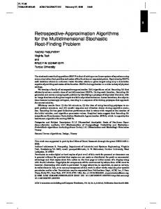
Reduce(f; �; �; �i for i = 1; : : :; k)
(7 + �)� ?1�?1 log(7m�?1 ). While jf j � � and f and ` are not �-optimal, For each edge vw, `(vw) e�f (vw) . Call FindPath(f; `; �) to nd an �-bad ow path P and a short path Q with the same endpoints as P. Reroute �i units of ow from P to Q. Return f.
�
Figure 1: Procedure Reduce. gradually update f until f and ` (de ned by the above formula) become �-optimal. Each update is done by choosing an �-bad ow path, rerouting some ow from this path to a much shorter path (with respect to `), and recomputing the length function. We will prove below that the parameter � in the de nition of length can be selected so that relaxed optimality condition R1 is always satis ed. Through iterative reroutings of ow, we gradually enforce relaxed optimality condition R2. When both relaxed optimality conditions are satis ed then Theorem 3.2 can be used to infer that f is �-optimal. For simplicity iof presentation, we shall assume for now that the value of the length function `(vw) = e�f (vw) at an edge vw can be computed in one step from f (vw) and represented in a single computer word. In Section 4.3 we will remove this assumption and sho that it is su�cient to compute an approximation to this value, and show that the time required for computing a su�ciently good approximation does not change the asymptotic running times of our algorithms. Procedure Reduce (see Figure 1), takes as input a multicommodity ow f , a target value � , an error parameter �, and a ow quantum �i for each commodity i. We require that each ow path comprising fi carries ow that is an integer multiple of �i . The procedure repeatedly reroutes �i units of ow from an �-bad path of commodity i to a shortest path. We will need a technical granularity condition that �i is small enough for every i to guarantee that approximate optimality is achievable through such reroutings. In particular, we assume that upon invocation of Reduce, for every commodity i we have
� �i � �2 102 log(7 m�?1 )
(3)
Upon termination, the procedure outputs an improved multicommodity ow f such that either jf j is less than the target value � or f is �-optimal. (Recall that we have assumed that � � 1=10.) In the remainder of this section, we analyze the procedure Reduce shown in Figure 1. First, we show that throughout Reduce f and ` satisfy relaxed optimality condition R1. Second, we show that if the granularity condition is satis ed, the number of iterations in Reduce is small. Third, we give an even smaller bound on the number of iterations for the case in which the ow f is O(�)optimal upon invocation of Reduce. This bound will be used in Section 5 to analyze an �-scaling algorithm presented there. Fourth, we describe e�cient implementations of procedure FindPath.
4.1 Bounding the number of iterations of Reduce
Lemma 4.1 If f is a multicommodity ow, and � � (7 + �)jf j?1�?1 log(7m�?1), then the multicommodity ow f and the length function `(vw) = e�f (vw) satisfy relaxed optimality condition R1.
Proof : Assume jf j ? f (v; w) � 7� f (v; w) for an edge vw 2 E and let �0 denote 7� . Observe that 8
j`j1 � e�jf j. Hence, we have j`j1 � e�jf j � e�jf j = e�jf j�0(1+�0 )?1 : `(v; w) e�f (v;w) e�jf j(1+�0)?1 We can use the bound on � in the statement of the lemma to conclude that this last term is at least 7m . Thus, `(vw) � � j`j1. � 7m At the beginning of Reduce, � is set equal to (7 + �)� ?1 �?1 log(7m�?1 ). As long as jf j � � , the value of � is su�ciently large, so by Lemma 4.1, relaxed optimality condition R1 is satis ed. If we are lucky and relaxed optimality condition R2 is also satis ed, then it follows that f and ` are �-optimal. Now we show that if R2 is not satis ed, then we can make signi cant progress. Like Shahrokhi and Matula, we use j`j1 as a measure of progress.
Lemma 4.2 Suppose �i and � satisfy the granularity condition. Then rerouting �i units of ow from an �-bad path of commodity i to the shortest path with the same endpoints decreases j`j1 by �
( minfD;kd (i)g j`j1 log m). i
Proof : Let P be an �-bad path from si to ti, and let Q be a shortest (si; ti)-path. Let A = P ? Q, and B = Q ? P . The only edges whose length changes due to the rerouting are those in A [ B . The decrease in j`j1 is `(A) + `(B ) ? e?�� `(A) ? e�� `(B ), which can also be written as i
i
(1 ? e?�� )(`(A) ? `(B )) ? (1 ? e?�� )(e�� ? 1)`(B ): i
i
i
The granularity condition, the de nition of �, and the assumption that � � 1=10, imply that 1 141 139 � x x ?x ��i � 7+ 102 � � �=7 � 1=70. For 0 � x � 70 , we have e � 1 + x, e � 1 + 140 x, and e � 1 ? 140 x.
Thus the decrease is at least 139 �� (`(A) ? `(B )) ? (�� ) � 141 �� � `(B ): i 140 i 140 i Now, observe that `(A) ? `(B ) is the same as `(P ) ? `(Q), and `(Q) = dist` (si ; ti). Also `(B ) � `(P ). This gives a lower bound of 139 �� (`(P ) ? dist (s ; t )) ? � 141 �2 � 2� `(P ): ` i i 140 i 140 i But P is �-bad, so this must be at least 139 �� (�0 `(P ) + �0 jf j 141 �2 � 2`(P ) j ` j ) ? i 1 140 minfD; kd(i)g 140 i �i j`j : = 139 ��i �0 `(P ) ? 141 �2 �i2`(P ) + 139 ��0 jf j 140 140 140 minfD; kd(i)g 1 � 0 We have seen that 7+ 102 � � ��i , which implies that 139� � 141��i and therefore the rst term dominates the second term. Thus the third term gives a lower bound on the decrease in j`j1. Substituting the value of � and using the fact that during execution of Reduce we have � � jf j, yields the claim of the lemma. The following theorem bounds the number of iterations in Reduce.
Theorem 4.3 If, for every commodity i, � and �i satisfy the granularity condition and jf j = O(� ) (i)g ) iterations. initially then the procedure Reduce terminates after O(�?1 maxi minfD;kd � i
9
Proof : Theorem 3.2 implies that if f and ` satisfy the relaxed optimality conditions then they are �-optimal. By Lemma 4.1, relaxed optimality condition R1 is maintained throughout all iterations. The fact that f is not yet �-optimal implies that condition R2 is not yet satis ed. Hence there exists an �-bad path for FindPath to nd. A single rerouting of ow from an �-bad path of commodity � ?1 i to a shortest path results in a reduction in j`j1 of at least ( minfD;kd (i)g j`j1 log(m� )). Since (i)g log?1 (m�?1 )) iterations reduce j`j by at least 1 ? x < e?x , it follows that every O(maxi minfD;kd 1 � i
a constant factor. Next we bound the number of times j`j1 can be reduced by a constant factor. Let f 0 denote the input multicommodity ow. For every edge0 vw, f 0 (vw) � jf 0j. Hence after we rst assign lengths to edges, the value of j`j1 is at most me�jf j . The length of every edge remains at least 1 so j`j1 is always at least m. Therefore, j`j1 can be reduced by a factor of e at most �jf 0 j times, which is O(�?1 log(m�?1 )) by the assumption that f = O(� ) and the value of �. This proves that Reduce terminated in the claimed number of iterations. i
Theorem 4.4 Suppose that the input ow f is O(�)-optimal, � and � satisfy the granularity condition, (i)g ) iterations. and jf j = O(� ) initially. Then the procedure Reduce terminates after O(maxi minfD;kd � i
Proof : Again let f 0 denote the input multicommodity ow. The assumption that f 0 is O(�)-optimal implies that jf 0j � (1 +?O (�))jf j for every multicommodity ow f . Therefore, the value of j`j1 is never less than e(1+O(�)) 1�jf 0j . As in Theorem 4.3, the initial value of j`j1 is at most me�jf 0j , so the number of times j`j1 can be reduced by a constant factor is O(��jf 0 j + log m), which is O(��jf 0 j) by
the choice of � and � . The theorem then follows as in the proof of Theorem 4.3.
4.2 Implementing an Iteration of Reduce We have shown that Reduce terminates after a small number of iterations. It remains to show that each iteration can be carried out quickly. Reduce consists of three steps|computing lengths, executing Findpath and rerouting ow. We discuss computing lengths in Section 4.3. In this section, we discuss the other two steps. We now consider the time taken by procedure FindPath. We will give three implementations of this procedure. First, we will give a simple deterministic implementation that runs in O(k� (m + P d(i) n log n) + n i � ) time, then a more sophisticated implementation that runs in time O(k� n log n + m(log n + min fk; k� log dmaxg)), and nally a randomized implementation that runs in expected O(�?1 (m + n log n)) time. All of these algorithms use the shortest-paths algorithm of Fredman and Tarjan [3] that runs in O(m + n log n) time. To deterministically nd a bad ow path, we rst compute, for every source node si , the length of the shortest path from si to every other node v . This takes O(k�(m + n log n)) time. In the simplest implementation we then compute the length of every ow path in P and compare its length to the P d(i) length of the shortest path to decide if the path is �-bad. There could be as many as �i � ow � P paths, each consisting of up to n edges, hence computing these lengths takes O n i d�(i) time. To decrease the time required for FindPath we have to nd an �-bad path, if one exists, without computing the length of so many paths. Observe that if there is an �-bad ow path for commodity i then the longest ow path for commodity i must be �-bad. Thus, instead of looking for an �-bad path in Pi for some commodity i, it su�ces to nd an �-bad path in the directed graph obtained by taking all ow paths in Pi , and treating the paths as directed away from si . In order to see if there is an �-bad path we need to compute the length of the longest path from si to ti in this directed graph. To facilitate this computation we shall maintain that the directed ow graph is acyclic. i
i
i
10
Let Gi denote the ow graph of commodity i. If Gi is acyclic, an O(m) time dynamic programming computation su�ces to compute the longest paths from si to every other node. Suppose that in an iteration we reroute ow from an �-bad path from si to ti , in the ow graph Gi . We must rst update the ow graph Gi to re ect this change. Second, the update might introduce directed cycles in Gi, so we must eliminate such cycles of ow. We use an algorithm due to Sleator and Tarjan [16] to implement this process. Sleator and Tarjan gave a simple O(nm) algorithm and a more sophisticated O(m log n) algorithm for the problem of converting an arbitrary ow into an acyclic ow. Note that eliminating cycles only decreases the ows on edges, so it cannot increase j`j1. Thus our bound on the number of iterations in Reduce still holds. We compute the total time required for each iteration of Reduce as follows. In order to implement FindPath, we must compute shortest path from si to ti in G and the longest path from si to ti in Gi for every commodity i, so the time required is O(k� (m + n log n) + km). Furthermore, after each rerouting, we must update the appropriate ow graph and eliminate cycles. Elimination of cycles takes O(m log n) time. Combining these bounds gives an O(k� n log n + m(k +log n)) bound on the running time of FindPath. In fact, further improvement is possible if we consider the ow graphs of all commodities with the same source and same ow quantum �i together. Let Gv;� be the directed graph obtained by taking the union of all ow paths P 2 Pi for a commodity i with si = v and �i = � , treating each path as directed away from v . If Gv;� is acyclic, an O(m) time dynamic programming computation su�ces to compute the longest paths from v to every other node in Gv;� . During our concurrent ow algorithm all commodities with the same demand will have same ow quantum. To limit the di�erent ow graphs that we have to consider we want to limit the number of di�erent demands. By decomposing demand d(i) into at most log d(i) demands with source si and sink ti we can assume that each demand is a power of 2. This way the number of di�erent ow graphs that we have to maintain is at most k� log dmax.
Lemma 4.5 The total time required for deterministically implementing an iteration of Reduce (assuming that exponentiation is a single step) is O(k�n log n + m(log n + min fk; k� log dmaxg)). Next, we give a randomized implementation of FindPath that is much faster when � is not too small; this implementation seems simple enough to be practical. If f and ` are not �-optimal, then relaxed optimality condition R2 is not satis ed, and thus �-bad paths contribute at least an � -fraction of the total sum P P i P 2P `(P )fi (P ). Therefore, by randomly choosing a ow path P 7 with probability proportional to its contribution to the above sum, we have at least an 7� chance of selecting an �-bad path. Furthermore, we will show that we can select a candidate �-bad path according to the right probability in O(m) time. Then we can compute a shortest path with the same endpoints in O(m + n log n) time. This enables us to determine whether or not P was an �-bad path. Thus we can implement FindPath in O(�?1 (m + n log n)) expected time. The contribution of a ow path P to the above sum is just the length of P times the ow on P , so we must choose P with probability proportional to this value. In order to avoid examining all such ow paths explicitly, we use a two-step procedure, as described in the following lemma. i
Lemma 4.6 If we choose an edge vw with probability proportional to `(vw)f (vw), and then we select a ow path among paths through this edge vw with probability proportional to the value of the ow carried on the path, thenPthePprobability that we have selected a given ow path P is proportional to its contribution to the sum i P 2P `(P )fi (P ). i
Proof : Let B =
P P
Select an edge vw with probability f (vw)`(vw)=B . Once an edge vw is selected, choose a path P 2 Pi through edge vw with probability ff((vwP )) . Consider a i
P 2Pi `(P )fi (P ).
i
11
commodity i and a path P 2 Pi .
Pr(P chosen) = =
X
vw2P
P) = Pr(vw chosen) � ff(i(vw )
`(wv)fi(P ) = fi (P )`(P ) : B B vw2P X
f (vw)`(vw) � fi (P ) B f (vw) vw2P X
Choosing an edge with probability proportional to `(vw)f (vw) can easily be done in O(m) time. In order to then choose with the right probability a ow path going through that edge, we need a data structure to organize these ow paths. For each edge we maintain a balanced binary tree with one leaf for each ow path through the edge, labeled with the ow value of that ow path. Each internal node of the binary tree is labeled with the total ow value of its descendent leaves. The number of paths is polynomial in n and �?1 , therefore using this data structure, we can randomly choose a ow path through a given edge in O(log n) time. In order to maintain this data structure, each time we change the ow on an edge, we must update the binary tree for that edge, at a cost of O(log n) time. In one iteration of Reduce the
ow only changes on O(n) edges, therefore the time to do these updates is O(n log n) per call to FindPath, which is dominated by the time to compute single-source shortest paths. We have shown that if relaxed optimality condition R2 is not satis ed, then, with probability of at least �=7, we can nd an �-bad path in O(m + n log n) time. FindPath continues to pick paths until either an �-bad path is found or 7=� trials are made. Observe that given that f and ` are not yet �-optimal (which implies that condition R2 is not yet satis ed), the probability of failure to nd an �-bad path in 7=� trials is bounded by 1=e. Thus, in this case, Reduce can terminate, claiming that f and ` are �-optimal with probability of at least 1 ? 1=e. Computing lengths and updating
ows can each be done in O(n log n) time, thus we get the following bound:
Lemma 4.7 One iteration of Reduce can be implemented randomly in time (�?1(m + n log n)) time (assuming that exponentiation is a single step).
The randomized algorithm as it stands is Monte Carlo; there is a non-zero probability that erroneously claims to terminate with an �-optimal f . To make the algorithm Las Vegas (never wrong, sometimes slow), we introduce a deterministic check. If FindPath fails to nd an �-bad path, Reduce computes the sum Pi dist` (si ; ti)d(i) to the required precision and compares it with jf jj`j1 to determine whether f and ` are really �-optimal. If not, the loop resumes. The time required to compute the sum is O(k� (m + n log n)), because at most k� single-source shortest path computations are required. The probability that the check must be done t times in a single call to ?1 t?1 , so the total expected contribution to the running time of Reduce is Reduce is at most (e ) � at most O(k (m + n log n)). (i)g , Recall that the bound on the number of iterations of Reduce is greater than maxi minfD;kd � which in turn is at least k. Since in each iteration we carry out at least one shortest path computation, the additional time spent on checking does not asymptotically increase our bound on the running time for Reduce. We conclude this section with a theorem summarizing the running time of Reduce for some cases of particular interest. For all of these bounds the running time is computed by multiplying the appropriate time for an iteration of Reduce by the appropriate number of iterations of Reduce. These bounds depend on the assumption that exponentiation is a single step. In Subsection 4.3 we Reduce
i
12
shall show that the same bounds can be achieved without this assumption. We shall also give a more e�cient implementation for the case when � is a constant. (i)g Theorem 4.8 Let f = O(� ) and � and �i satisfy the granularity condition. Let H (k; d; �) = maxi minfD;kd � and let k^ = min fk; k� log dmaxg. Then the following table contains running times for various implemeni
tations of procedure Reduce (assuming that exponentiation is a single step).
Randomized Implementation Deterministic Implementation � � ? � 1 � � � poly1(n) O �?2 (m + n log n)H(k; d; �) O �?1H(k; d; �)[k�n logn + m(log n + k^)] � � ? � 1 � � � poly1(n) , O �?1 (m + n log n)H(k; d; �) O H(k; d; �)[k�n logn + m(log n + k^)] f is O(�)-opt.
4.3 Further implementation details In this section, we will show how to get rid of the assumption that exponentiation can be performed in a single step. We will also give a more e�cient implementation of the procedure Reduce for the case when � is xed.
4.3.1 Removing the assumption that exponentiation can be performed in O(1) time To remove the assumption that exponentiation can be performed in O(1) time, we will need to do two things. First we will show that it is su�cient to work with edge-lengths `^(vw) that are approximations to the actual lengths `(vw) = e�f (vw). We then show that computing these approximate edge-lengths does not change the asymptotic running times of our algorithms. The rst step is to note that in the proof of Lemma 4.2, we never used the fact that we reroute
ow onto a shortest path. We only need that we reroute ow onto a su�ciently short path. More precisely, it is easy to convert the proof of Lemma 4.2 into a proof for the following claim.
Lemma 4.9 Suppose �i and � satisfy the granularity condition and let P be a ow path of commodity
i. Let Q be a path connecting the endpoints of P such that the length of Q is no more than �0 `(P )=2 + �0 jDf j j`j1=2 greater than the length of the shortest path connecting the same endpoints. Then rerouting � �i units of ow from path P to Q decreases j`j1 by ( minfD;kd (i)g j`j1 log m)). i
We will now show that in order to compute the lengths of paths up to the precision given in this lemma, we only need to compute the lengths of edges up to a reasonably small amount of precision. By Lemma 4.9, the length of a path can have a rounding error of �0 jDf j j`j1=2. Each path has at most n edges, so it will su�ce to ensure that each edge has a rounding error of n1 (�0 jDf j j`j1=2). We will now bound this quantity. jf j is the maximum
ow on an edge and hence must be at least as large P as the average ow on an edge, i.e. jf jP� vw f (vw)=m. Every unit of ow contributes to the total
ow on at least one edge, and hence vw f (vw) � D and combining with the previous equation, we get that jf j=D � 1=m. j`j1 is at least as big as the length of the longest edge, i.e. 0 j`j1 � e�jf j. � e�jf j. Each Plugging in these bounds we see that it su�ces to compute with an error of at most nm edge has a positive length of at most e�0jf j and can be expressed as e�jf j�, where 0 < � � 1. Thus we � . To do so, we need to compute O(log(�?1 nm)) bits which need to compute � up to an error of nm by the assumption that � is inverse polynomial in n is just O(log n) bits. By using the Taylor series expansion of ex , we can compute one bit of the length function in O(1) time. Therefore, to compute the lengths of all edges at each iteration of Reduce, we 13
need O(m log n) time. In the deterministic implementation of Reduce each iteration takes at least
(m log n) time (the time required for cycle cancelling), therefore the time spent on computing the lengths is dominated by the running time of an iteration. The approximation above depends on the current value of jf j, which may change after each iteration. It was crucial that we recomputed the lengths of every edge in every iteration. The time to do so, O(m log n), would dominate the running time of the randomized implementation of Reduce. (Recall that the randomized implementation does not do cycle cancelling.) Thus, we need to nd an approximation which does not need to be recomputed at every iteration. We will choose one which does not depend on the current jf j and hence will only need to be updated on the O(n) edges on which the ow actually changes. We proceed to describe such an approximation which will depend on � rather than jf j. Throughout Reduce all edge length are at most eO(�� ), and at least one edge has length more than e�� . Therefore, j`j1 is at least e�� , and by the same argument as for the deterministic case O(�?1 log n) bits of precision su�ce throughout Reduce. When we rst call Reduce, we must spend O(�?1 m log n) time to compute all the edge lengths. For each subsequent iteration, we only need to spend O(�?1 n log n) time updating the O(n) edges whose length has changed. Since each iteration of Reduce is expected to take O(�?1 (m + n log n)) time to compute shortest paths in FindPath, the time for updating edges is dominated by the time required by FindPath. While it appears that the time to initially compute all the edge lengths may dominate the time spent in one invocation of Reduce, we shall see in Section 5 that whenever any of our algorithms calls Reduce, it will have at least (log n) iterations. Each iteration is expected to take at least (�?1 m) time to compute the shortest paths in FindPath. Therefore, the time spent on initializing lengths will be dominated by the running time of Reduce. Note that in describing the randomized version of FindPath in Lemma 4.6, we assumed we knew the exact lengths. However, by usingPthe approximate lengths we do not signi cantly change a P path's apparent contribution to the sum i P 2P `(P )fi (P ). Hence we do not signi cantly reduce the probability of selecting a bad path. Thus we have shown that without any assumptions, Reduce can be implemented deterministically in the same time as is stated in Theorem 4.8. Although for the randomized version, there is additional initialization time, for all the algorithms in this paper that initialization time is dominated by the time spent in the iterations of Reduce. i
Theorem 4.10 The times required for the deterministic implementations of procedure Reduce stated in Theorem 4.8 hold without the assumption that exponentiation is a single step. The time required by the randomized implementations increases by an additive factor of O(�?1 m log n) without this assumption. 4.3.2 Further improvements for xed � In this section we show how one can reduce the time per iteration of Reduce for the case in which � is a constant. First we show how using approximate lengths can reduce the time required by FindPath; we use an approximate shortest-paths algorithm that runs in O(m + n�?1 ) time. Then we give improved implementation details for an iteration of Reduce to decrease the time required by other parts of Reduce. We will describe how, given the lengths and an �-bad path P from s to t, we can nd a path Q with the same endpoints such that `(Q) � dist` (s; t) + �0 `(P )=2 in O(m + n�?1 ) time. First, we discard all edges with length greater than `(P ), for they can never be in a path that is shorter than P (if P is a shortest path between s and t then P is not an �-bad path). Next, on0 the remaining graph, we compute shortest paths from s using approximate edge-lengths `~(v; w) = � `2(nP ) d`(vw) �0 `2(nP ) e, thus 14
giving us dist`~(s; t), an approximation of dist` (s; t), the length of the actual shortest (s; t)-path. There are at0 most n ? 1 edges on any shortest path, and for each such edge, the approximate length is at most � `2(nP ) more than the actual length. Thus we know that 0 0 dist`~(s; t) � dist` (s; t) + n � `2(nP ) = dist` (s; t) + � `(2P ) 0 Further, since each shortest path length is an integer multiple of � `2(nP ) , and no more than `(P ), we can use Dial's implementation of Dijkstra's algorithm [2] to compute dist`~(s; t) in O(m + n�?1 ) time. Implementing FindPath with this approximate shortest path computation directly improves the time required by a deterministic implementation of Reduce. The randomized implementation of ?1 ?1 FindPath with approximate shortest path computation requires O(� (m + n� )) expected time. In order to claim that an iteration of Reduce can be implemented in the same amount of time, we must handle two di�culties, updating edge lengths and updating each edge's table of ow paths when ow is rerouted. Previously, these steps took O(n log n) time, which was dominated by the time for FindPath. We have reduced the time for FindPath, so the time for these steps now dominates. We show how to carry out these steps in O(n) time. For the rst step, we show that a table can be precomputed so that each edge length can be updated in constant time. For the second step, we sketch a three-level data structure that allows selection of a random ow path through an edge in O(n) time, and allows constant-time addition and deletion of ow paths. Say that before computing the length e�f (vw), we were to round �f (vw) to the nearest multiple of �=c, for some constant c. This will introduce an additional multiplicative error of 1 + O(�=c) in the length of each edge and hence an additional multiplicative error of 1 + O(�=c) on each path. However, by arguments similar to the previous subsection, this will still give us a su�ciently precise approximation. Now we will show, that by rounding in this way there are a small enough number of possible values for `(vw) that we can just compute them all at the beginning of an iteration of Reduce and then compute the length of an edge by simply looking up the value in a precomputed table. The largest value of �f (vw) we ever encounter is O(�?1 log n). Since we are only concerned with multiples of �=c, there are a total of only O(�?2 log n) values, we will ever encounter. At the beginning of each iteration, we can compute each of these numbers to a precision of O(log n) bits in O(�?2 log2 n) time. Once we have computed all these numbers, we can compute the length of an edge by computing �f (vw), truncating to a multiple of �=c and then looking up the value of `(vw) in the table. This takes O(1) time. Thus for constant �, we are spending O(log2 n + m) = O(m) time per iteration. Now we address the problem of maintaining, for each edge, the ow paths going through that edge. Henceforth we will describe the data structure associated with a single edge. First suppose that all the ow paths carry the same amount of ow, i.e. �i is the same for each. In this case, we keep pointers to the ow paths in an array. We maintain that the array is at most one-quarter empty. It is then easy to randomly select a ow path in constant expected time; one randomly chooses an index and checks whether the corresponding array entry has a pointer to a ow path. If so, select that ow path. If not, try another index. One can delete ow paths from the array in constant time. If one maintains a list of empty entries, one can also insert in constant time. If the array gets too full, copy its contents into a new array of twice the size. The time required for copying can be amortized over the time required for the insertions that lled the array. If the array gets too empty, copy its contents into a new array of half the size. The time required for copying can be amortized over the time required for the deletions that emptied the array. (See, for example, [1], for a detailed description of this data structure.) Now we consider the more general case, in which the ow values of ow paths may vary. In this case, we use a three-level data structure. In the top level, the paths are organized according to their 15
starting nodes. In the second level, the paths with a common starting node are organized according to their ending nodes. The paths with the same starting and ending nodes may be assumed to belong to the same commodity and hence all carry the same amount of ow. Thus these paths can be organized using the array as described above. The rst level consists of a list; each list item speci es a starting node, the total ow of all ow paths with that starting node, and a pointer to the second-level data structure organizing the ow paths with the given starting node. Each second-level data structure consists of a list; each list item speci es an ending node, the total ow of all ow paths with that ending node and the given starting node, and a pointer to the third-level data structure, the array containing ow paths with the given starting and ending nodes. Now we analyze the time required to maintain this data structure. Adding and deleting a ow path takes constant time. Choosing a random ow path with the right probability can be accomplished in O(n) time. First we randomly choose a value between 0 and the total ow through the edge. Then we scan the rst-level list to select an appropriate item based on the value. Next we scan the second-level list pointed to by that item, and select an item in the second-level list. Each of these two steps takes O(n) time. Finally, we select an entry in the third-level array. In the third level array, all the ows have the same �i , thus this can be accomplished in O(1) expected time by the scheme described above. So we have shown that for constant �, each of the three steps in procedure Reduce can be implemented in O(m) expected time, thus yielding the following theorem.
Theorem 4.11 Let f = O(� ) and � and �i satisfy the granularity condition. Let H (k; d; �) = (i)g and let k^ = min fk; k� log d g. For any constant � > 0 the procedure Reduce can maxi minfD;kd max �
be implemented in randomized O(mH (k; d; �)) and in deterministic O(H (k; d; � )m(log n + k^)) time. i
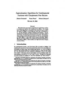
5 Concurrent ow algorithms In this section, we give approximation algorithms for the concurrent ow problem with uniform capacities. We describe two algorithms: Concurrent and ScalingConcurrent. Concurrent is simpler and is best if � is constant. ScalingConcurrent gradually scales � to the right value, and is faster for small �. Algorithm Concurrent (see Figure 2) consists of a sequence of calls to procedure Reduce described in the previous section. The initial ow is constructed by routing each commodity i on a single ow path from si to ti . Initially, we set �i = d(i). Before each call to Reduce we divide the
ow quantum �i by 2 for every commodity where this is needed to satisfy the granularity condition (3). Each call to Reduce modi es the multicommodity ow f so that either jf j decreases by a factor of 2 or f becomes �-optimal. (The procedure Reduce can set a global ag to indicate whether it has concluded that f is �-optimal.) In the latter case our algorithm can terminate and return the
ow. As we will see, O(log m) calls to Reduce will su�ce to achieve �-optimality.
Theorem 5.1 The algorithm Concurrent nds an �-optimal multicommodity ow in O((�?1 k + �?3 m)(k�n log n + m(log n + minfk; k� log dmaxg)) log n), or in expected time
O((k�?2 + m�?4 )(m + n log n) log n).
Proof : Immediately after the initialization we have jf j � D. To bound the number of phases we need a lower bound on the minimum value of jf j. Observe that for every multicommodity ow f ,
the total amount of ow in the network is D. Every unit of ow contributes to the total ow on at 16
Concurrent(G; �; fd(i); (si ; ti) : 1 � i � kg)
For each commodity i: �i d(i), create a simple path from si to ti and route d(i) ow on it. � jf j=2. While f is not �-optimal, For every i, Until �i and � satisfy the granularity condition, �i �i=2. Call Reduce(f; �; �; d). � �=2. Return f.
Figure 2: Procedure Concurrent. P
least one of the edges, and hence vw2E f (vw) � D. Therefore,
jf j � D=m:
(4)
This implies that the number of iterations of the main loop of Concurrent is at most O(log m). By Theorems 4.3 and 4.8, procedure Reduce invoked during a single iteration of Concurrent (i)g ) iterations. rst spends O(m log n) time initializing edge lengths and then executes O(�?1 minfD;kd � Throughout the algorithm �i is either equal to d(i), or is �(�2 �= log(m�?1 )) for every i. In the rst case, min fD; kd(i)g = min fD; kd(i)g = min � D ; k� � k: �i d(i) d(i) In the second case min fD; kd(i)g = min fD; kd(i)g �?2 � ?1 log(m�?1 ) � �?2 D log(m�?1 ): i
�i
� Thus the total number of iterations of the loop of Reduce is at most O(�?1 (k + �?2 D� log(m�?1 )), and the time spent on the initialization the edge length is dominated. The value � is halved at every iteration, therefore the total number of calls required for all iterations is at most O(�?1 k log n) plus twice the number required for the last iteration of Concurrent. It follows from (4) that � is ( mD ), and the total number of iterations of the loop of Reduce is at most O(�?1 k log n + �?3 m log n). Consider the special case when � is constant. We use the version of Reduce implemented with
an approximate shortest path computation, and apply the bounds of Theorem 4.11 combined with a proof similar to that of Theorem 5.1 to get the following result:
Theorem 5.2 For any constant � > 0, an �-optimal solution for the unit-capacity concurrent ow
problem can be found in O(m(k + m) log2 n) expected time by a randomized algorithm and in O(m(k + m)(log n + min fk; k� log dmaxg) log n) time by a deterministic algorithm.
If � is less than a constant, we use the algorithm ScalingConcurrent, shown in Figure 3. It starts with a large �, and then gradually scales � down to the required value. More precisely, algorithm ScalingConcurrent starts by applying algorithm Concurrent with � = 101 . ScalingConcurrent then repeatedly divides � by a factor of 2 and calls Reduce. After the initial call to Concurrent, f is 101 -optimal, i.e. jf j is no more than twice the minimum possible value. Therefore, jf j cannot be decreased below �=2, and every subsequent call to Reduce returns an �-optimal multicommodity ow (with the current value of �). As in Concurrent, each call to Reduce uses the largest ow quantum � permitted by the granularity condition (3). 17
ScalingConcurrent(G; �0 ; fd(i); (si ; ti) : 1 � i � kg)
� 101 . Call Concurrent(G; �; fd(i); (si ; ti) : 1 � i � kg), and let f be the resulting ow. � �=2.
While � > �0, � �=2, For every i, Until �i and � satisfy the granularity condition, �i �i=2. Call Reduce(f; �; �; �). Return f.
Figure 3: Procedure ScalingConcurrent.
Theorem 5.3 The algorithm ScalingConcurrent nds an �-optimal multicommodity ow in expected time O((k�?1 + m�?3 log n)(m + n log n)).
Proof : As is stated in Theorem 5.2, the call to procedure Concurrent takes O(km log n+m2 log m) time, and returns a multicommodity ow f that is 101 -optimal, hence jf j is no more than twice the
minimum. Therefore every subsequent call to Reduce returns an �-optimal multicommodity ow f . The time required by one iteration is dominated by the call to Reduce. The input ow f of Reduce is 2�-optimal, so, by Theorems 4.8 and 4.10, the time required by the randomized imple(i)g ). We have seen that max minfD;kd(i)g is mentation of Reduce is O(�?1 (m + n log n) maxi minfD;kd i � � at most O(k + �?2 m log m). The value of � is reduced by a factor of two in every iteration. Therefore, the total time required for all iterations is at most twice the time required by the last iteration. The last iteration takes O((k + �?2 m log n)(�?1 (m + n log n))) time, which proves the claim. Consider an implementation of Concurrent or ScalingConcurrent with the deterministic version of Reduce. The time required by FindPath does not depend on �, so we can not claim that the time is bounded by at most twice the time required for the last call to Reduce. Since there are at most log �?1 iterations, we have the following theorem. i
i
Theorem 5.4 An �-optimal solution to the unit-capacity concurrent ow problem can be found deterministically in time O(km log2 n +(k log �?1 + �?2 m log n)(k�n log n + m(log n +min fk; k� log dmaxg))).
6 Two applications In this section we describe two applications of our unit-capacity concurrent ow algorithm. The rst application is to e�ciently implement Leighton and Rao's sparsest cut approximation algorithm [11], and the second application is to approximately minimize channel width in VLSI routing; the second problem was considered by Raghavan and Thompson [13] and Raghavan [12]. We start by reviewing the result of Leighton and Rao concerning nding an approximately sparsest cut in a graph. For any partition of the nodes of a graph G into two sets A and B , the associated cut is the set of edges between A and B , and � (A; B ) denotes the number of edges in that cut. A cut is sparsest if � (A; B )=(jAjjB j) is minimized. Leighton and Rao [11] gave an O(log n)-approximation algorithm for nding the sparsest cut of a graph. By applying this algorithm they obtained polylogtimes-optimal approximation algorithms for a wide variety of NP-complete graph problems, including 18
minimum feedback arc set, minimum cut linear arrangement, and minimum area layout. Leighton and Rao exploited the following connection between sparsest cuts and concurrent ow. Consider an all-pairs multicommodity ow in G, where there is a unit of demand between every pair of nodes. In a feasible ow f , for any partition A [ B of the nodes of G, a total of at least jAjjBj units of ow must cross the cut between A and B. Consequently, one such edge must carry at least jAjjB j=� (A; B ) ow for the sparsest cut A [ B . Leighton and Rao prove an approximate max- ow, min-cut theorem for the all-pairs concurrent ow problem, by showing that in fact this lower bound for jf j is at most an O(log n) factor below the minimum value. Their approximate sparsest-cut algorithm makes use of this connection. More precisely given a nearly optimal length function (dual variables) they show how to nd a partition A [ B that is within a factor of O(log n) of the minimum value of jf j, and hence of the value of the sparsest cut.1 The computational bottleneck of their method is solving a unit-capacity concurrent ow problem, in which there is a demand of 1 between every pair of nodes. In their paper, they appealed to the fact that concurrent ow can be formulated as a linear program, and hence can be solved in polynomial time. A much more e�cient approach is to use our unit-capacity approximation algorithm. The number of commodities required is O(n2 ). Leighton [10] has discovered a technique to reduce the number of commodities required. He shows that if the graph in which there is an edge connecting each source-sink pair is an expander graph, then the resulting ow problem su�ces for the purpose of nding an approximately sparsest cut. (We call this graph the demand graph.) In an expander we have: For any partition of the node set into A and B , where jAj � jB j, the number of commodities crossing the associated cut is �(jAj). Therefore the value of jf j for this smaller ow problem is (jAj=� (A; B )). Since jB j � n=2, it follows that njf j is (jAjjB j)=� (A; B )). The smaller ow problem essentially \simulates" the original all-pairs problem. Moreover, Leighton and Rao's sparsest-cut algorithm can start with the length function for the smaller ow problem in place of that for the all-pairs problem. Thus Leighton's idea allows one to nd an approximate sparsest-cut after solving a much smaller concurrent ow problem. If one is willing to tolerate a small probability of error in the approximation, one can use O(n) randomly selected source-sink pairs for the commodities. It is well known how to randomly select node pairs so that, with high probability, the resulting demand graph is an expander. By Theorem 5.2, algorithm Concurrent takes expected time O(m2 log2 m) to nd an appropriate solution for this smaller problem.
Theorem 6.1 An O(log n)-factor approximation to the sparsest cut in a graph can be found by a randomized algorithm in O(m2 log2 m) time.
The second application we discuss is approximately minimizing channel width in VLSI routing. Often a VLSI design consists of a collection of modules separated by channels; the modules are connected up by wires that are routed through the channels. For purposes of regularity the channels have uniform width. It is desirable to minimize that width in order to minimize the total area of the VLSI circuit. Raghavan and Thompson [13] give an approximation algorithm for minimizing the channel width. They model the problem as a graph problem in which one must route wires between pairs of nodes in a graph G so as to minimize the maximum number of wires routed through an edge. To approximately solve the problem, they rst solve a concurrent ow problem where there is a commodity with demand 1 for each path that needs to be routed. An optimal solution fopt fails 1 Their algorithm also works for edge-weighted graphs; weights translate to edge capacities in the corresponding concurrent ow problem.
19
to be a wire routing only in that it may consist of paths of fractional ow. However, the value of
jfoptj is certainly a lower bound on the minimum channel width. Raghavan and Thompson give a randomized method for converting the fractional ow fopt to an integral ow, increasing the channel width only slightly. The resulting wire routing f achieves channel width q
jf j � jfoptj + O( jfoptj log n) p which is at most w + O( w log n), where w
(5)
min min is the minimum width. In fact, the constant min implicit in this bound is quite small. Later Raghavan [12] showed how this conversion method can be made deterministic. The computational bottleneck is, once again, solving a unit-capacity concurrent ow problem. Theorems 5.3 and 5.4 are applicable, and yield good algorithms. But if wmin is (log n), we can do substantially better.2 In this case, a modi ed version of our algorithm ScalingConcurrent directly yields an integral f satisfying (5), although the big-Oh constant is not as good as that of [13]. Consider the procedure ScalingConcurrent. It consists of two parts. First the procedure 1 1 Concurrent is called with � = 10 to achieve 10 -optimality. Next, ScalingConcurrent repeatedly calls Reduce, reducing the error parameter � by a factor of two every iteration, till the required accuracy is achieved. The demands are the same for every commodity, hence �i is independent of i, and we shall denote it by � . We claim that if wmin = (log n) then � , which is initially 1 for this application, need never be reduced. Consequently, there remains a single path of ow per commodity, and the randomized conversion method of Raghavan and Thompson p becomes unnecessary. We show that these paths constitute a routing with width wmin + O( wmin log n). First suppose the call to Concurrent terminates because the granularity condition becomes false. At this point, we have that
1 > �2 �=(51 log(7m�?1 )):
(6)
We have that � � jf j=2 and � = 101 ,pand therefore jf j = O(log n). By our assumption that wmin =
(log n), and hence jf j � wmin + O( wmin log n). Now assume that the call to Concurrent terminates with a 101 -optimal ow. We proceed with ScalingConcurrent. It terminates when the granularity condition becomes false, at which point inequality (6) implies that �2 = O((log m)=� ). The ow f is �-optimal and integral. Sopjf j � wmin + p O(wmin (log m)=� ). Since � = jf j=2 � wmin=2, this bound on jf j is at most wmin + O( wmin log m), as required.
Theorem p6.2 If wmin denotes the minimum possible width and wmin = (log m), a routing of width wmin + O( wminplog n) can be found by a randomized algorithm in expected time O(km log n log k + k3=2(m+n log n)= log n), and by a deterministic algorithm in time O(k log k(k�n log n+mk� +m log n)). Proof : We have shown that algorithm ScalingConcurrent nds the required routing if it is
terminated as soon as the granularity condition becomes false with � = 1. Now we analyze the time required. We have D = k and d(i) = 1 for every i, and throughout the algorithm we have �i = 1 for every i. The number of calls to Reduce during Concurrent is O(log k) (initially jf j � k, and it never gets below 1 with � = 1). Therefore the number iterations of the loop of Reduce required during 2 This
is the case of most interst, for if wmin is o(log n), then the error term in (5) dominates wmin.
20
is O(k log k). Next we proceed with ScalingConcurrent. The number of iterations is at most O(log k), because � is reduced by a factor of two each iteration, � starts at 101 and never gets below 1=k. Each iteration is a call to Reduce, which in turn results in O(k) iterations of the loop of Reduce. The time required by one iteration of the loop deterministically is O(k� n log n + m(k� + log m)), and the total time to nd a good routing of wires is O(k log k(k� n log n + mk� + m log n)). The expected time required by the randomized implementation of Reduce is O(m log n + ? 1 k� (m + n log n)). The total expected time required by Concurrent is O(mk log k log n). After the call to Concurrent � decreases by a factor of two each iteration, it follows that the total expected time required for all iterations is O(m log n logp�?1 ) plus twice the time for the last call to Reduce. During the last call to Reduce, �?1 = O( k= log n), so the time required for all iterp ations is O(km log n log k + k3=2(m + n log n)= log n). This time dominates the time required by Concurrent since wmin = (log n) implies k = (log n). Concurrent
Acknowledgments We are grateful to Andrew Goldberg, Tom Leighton, Satish Rao, David Shmoys, and Pravin Vaidya for helpful discussions.
References [1] Thomas H. Cormen, Charles E. Leiserson, and Ronald L. Rivest. Introduction to Algorithms. MIT Press/McGraw-Hill, 1990, pp. 367-375. [2] R. Dial. Algorithm 360: Shortest path forest with topological ordering. Communications of the ACM, 12:632{633, 1969. [3] M.L. Fredman and R.E. Tarjan. Fibonacci heaps and their uses in improved network optimization algorithms. Journal of the ACM, 34:596{615, 1987. [4] A. V. Goldberg and R. E. Tarjan. Solving minimum-cost ow problems by successive approximation. Mathematics of Operations Research, 15(3):430{466, 1990. [5] M. D. Hansen. Approximation algorithms for geometric embeddings in the plane with applications to parallel processing problems. In Proceedings of the 30th Annual Symposium on Foundations of Computer Science, pages 604{610. IEEE, October 1989. [6] S. Kapoor and P. M. Vaidya. Fast algorithms for convex quadratic programming and multicommodity ows. In Proceedings of the 18th Annual ACM Symposium on Theory of Computing, pages 147{159, 1986. [7] P. Klein, A. Agrawal, R. Ravi, and S. Rao. Approximation through multicommodity ow. In Proceedings of the 31st Annual Symposium on Foundations of Computer Science, pages 726{727, 1990. [8] P. Klein and C. Stein. Leighton-Rao might be practical: a faster approximation algorithm for uniform concurrent ow. Unpublished manuscript, November 1989. [9] P. Klein, C. Stein, and E� . Tardos. Leighton-Rao might be practical: faster approximation algorithms for concurrent ow with uniform capacities. In Proceedings of the 22nd Annual ACM Symposium on Theory of Computing, pages 310{321, May 1990. 21
[10] F. T. Leighton, November 1989. Private communication. [11] T. Leighton and S. Rao. An approximate max- ow min-cut theorem for uniform multicommodity
ow problems with applications to approximation algorithms. In Proceedings of the 29th Annual Symposium on Foundations of Computer Science, pages 422{431, 1988. [12] P. Raghavan. Probabilistic construction of deterministic algorithms: approximating packing integer programs. In Proceedings of the 27th Annual Symposium on Foundations of Computer Science, pages 10{18, 1986. [13] P. Raghavan and C. D. Thompson. Provably good routing in graphs: regular arrays. In Proceedings of the 17th Annual ACM Symposium on Theory of Computing, pages 79{87, 1985. [14] R. Ravi, A. Agrawal, and P. Klein. Ordering problems approximated: single-processsor scheduling and interval graph completion. In Proceedings of the 1989 ICALP Conference, 1991. To appear. [15] F. Shahrokhi and D. W. Matula. The maximum concurrent ow problem. Journal of the ACM, 37:318 { 334, 1990. [16] D. D. Sleator and R. E. Tarjan. A data structure for dynamic trees. Journal of Computer and System Sciences, 26:362{391, 1983. [17] E. Tardos. Improved approximation algorithm for concurrent multi-commodity ows. Technical Report 872, School of Operations Research and Industrial Engineering, Cornell University, October 1989. [18] P. M. Vaidya. Speeding up linear programming using fast matrix multiplication. In Proceedings of the 30th Annual Symposium on Foundations of Computer Science, pages 332{337, 1989.
22