Faster Gradient Descent Training of Hidden Markov Models, Using ...

Faster Gradient Descent Training of Hidden Markov Models, Using Individual Learning Rate Adaptation Pantelis G. Bagos, Theodore D. Liakopoulos, and Stavros J. Hamodrakas Department of Cell Biology and Biophysics, Faculty of Biology, University of Athens Panepistimiopolis, Athens 15701, Greece {pbagos,liakop}@biol.uoa.gr, [email protected]

Abstract. Hidden Markov Models (HMMs) are probabilistic models, suitable for a wide range of pattern recognition tasks. In this work, we propose a new gradient descent method for Conditional Maximum Likelihood (CML) training of HMMs, which significantly outperforms traditional gradient descent. Instead of using fixed learning rate for every adjustable parameter of the HMM, we propose the use of independent learning rate/step-size adaptation, which has been proved valuable as a strategy in Artificial Neural Networks training. We show here that our approach compared to standard gradient descent performs significantly better. The convergence speed is increased up to five times, while at the same time the training procedure becomes more robust, as tested on applications from molecular biology. This is accomplished without additional computational complexity or the need for parameter tuning.

1 Introduction Hidden Markov Models (HMMs) are probabilistic models suitable for a wide range of pattern recognition applications. Initially developed for speech recognition [1], during the last few years they became very popular in molecular biology for protein modeling [2,3] and gene finding [4,5]. Traditionally, the parameters of an HMM (emission and transition probabilities) are optimized according to the Maximum Likelihood (ML) criterion. A widely used algorithm for this task is the efficient Baum-Welch algorithm [6], which is in fact an Expectation-Maximization (EM) algorithm [7], guaranteed to converge to at least a local maximum of the likelihood. Baldi and Chauvin later proposed a gradient descent method capable of the same task, which offers a number of advantages over the Baum-Welch algorithm, including smoothness and on-line training abilities [8]. When training an HMM using labeled sequences [9], we can either choose to train the model according to the ML criterion, or to perform Conditional Maximum Likelihood (CML) training which is shown to perform better in several applications [10]. ML training could be performed (after some trivial modifications) with the use of standard techniques such as the Baum-Welch algorithm or gradient descent, whereas for CML training one should rely solely on gradient descent methods. The main advantage of the Baum-Welch algorithm (and hence the ML training) is due to its simplicity and the fact that requires no parameter tuning. Furthermore comG. Paliouras and Y. Sakakibara (Eds.): ICGI 2004, LNAI 3264, pp. 40–52, 2004. © Springer-Verlag Berlin Heidelberg 2004

Faster Gradient Descent Training of Hidden Markov Models

41

pared to standard gradient descent, even for ML training, the Baum-Welch algorithm achieves significantly faster convergence rates [11]. On the other hand gradient descent (especially in the case of large models) requires careful search in the parameter space for an appropriate learning rate in order to achieve the best possible performance. In the present work, we extend the gradient descent approach for CML training of HMMs. We then, adopting ideas from the literature regarding training techniques applied on feed-forward back-propagated multilayer perceptrons, introduce a new scheme for gradient descent optimization for HMMs. We propose the use of independent learning rate/step-size adaptation for every trainable parameter of the HMM (emission and transition probabilities), and we show that not only outperforms significantly the convergence rate of the standard gradient descent, but also leads to a much more robust training procedure whereas at the same time it is equally simple enough, since it requires almost no parameter tuning. In the following sections we will first establish the appropriate notation for describing a Hidden Markov Model with labeled sequences, following mainly the notation used in [2] and [12]. We will then briefly describe the algorithms for parameter estimation with ML and CML training and afterwards we will introduce our proposal, of individual learning rate adaptation as a faster and simpler alternative to standard gradient descent. Eventually, we will show the superiority of our approach on a real life application from computational molecular biology, training a model for the prediction of the transmembrane segments of β-barrel outer membrane proteins.

2 Hidden Markov Models A Hidden Markov Model is composed of a set of (hidden) states, a set of observable symbols and a set of transition and emission probabilities. Two states k, l are connected by means of the transition probabilities αkl, forming a 1st order Markovian process. Assuming a protein sequence x of length L denoted as: x = x1 , x2 ,..., xL

(1)

where the xi’s are the 20 amino acids, we usually denote the “path” (i.e. the sequence of states) ending up to a particular position of the amino acid sequence (the sequence of symbols), by π. Each state k is associated with an emission probability ek(xi), which is the probability of a particular symbol xi to be emitted by that state. When using labeled sequences, each amino acid sequence x is accompanied by a sequence of labels y for each position i in the sequence: y = y1 , y2 ,..., y L

(2)

Consequently, one has to declare a new probability distribution, in addition to the transition and emission probabilities, the probability ∆k(c) of a state k having a label c. In almost all biological applications this probability is just a delta-function, since a

42

Pantelis G. Bagos, Theodore D. Liakopoulos, and Stavros J. Hamodrakas

particular state is not allowed to match more than one label. The total probability of a sequence x given a model is calculated by summing over all possible paths: P ( x | θ ) = ∑ P ( x , π | θ ) = ∑ a0 π π

π

1

∏e

πi

( xi ) aπ π i

i =1

(3)

i +1

This quantity is calculated using a dynamic programming algorithm known as the forward algorithm, or alternatively by the similar backward algorithm [1]. In [9] Krogh proposed a simple modified version of the forward and backward algorithms, incorporating the concept of labeled data. Thus we can also use, the joint probability of the sequence x and the labeling y given the model: P ( x, y | θ ) =

∑ P ( x, y,π | θ ) = ∑ P ( x,π | θ ) = ∑ a ∏ e 0π 1

π

π ∈Π y

π ∈Π y

πi

( xi ) aπ π i

i +1

(4)

i =1

The idea behind this approach is that summation has to be done only over those paths Πy that are in agreement with the labels y. If multiple sequences are available for training (which is usually the case), they are assumed independent, and the total likelihood of the model is just a product of probabilities of the form (3) and (4) for each of the sequences. The generalization of Equations (3) and (4) from one to many sequences is therefore trivial, and we will consider only one training sequence x in the following. 2.1 Maximum Likelihood and Conditional Maximum Likelihood The Maximum Likelihood (ML) estimate for any arbitrary model parameter, is denoted by:

θ

ML

= arg max P ( x | θ ) θ

(5)

The dominant algorithm for ML training is the elegant Baum-Welch algorithm [6]. It is a special case of the Expectation-Maximization (EM) algorithm [7], proposed for Maximum Likelihood (ML) estimation for incomplete data. The algorithm, updates iteratively the model parameters (emission and transition probabilities), using their expectations, computed with the use of forward and backward algorithms. Convergence to at least a local maximum of the likelihood is guaranteed, and since it requires no initial parameters, the algorithm needs no parameter tuning. It has been shown, that maximizing the likelihood with the Baum-Welch algorithm can be done equivalently with a gradient descent method [8]. It should be mentioned here, as it is apparent from the above equations where the summation is performed over the entire training set, that we consider only batch (off-line) mode of training. Gradient descent could also be performed on on-line mode, but we will not consider this option in this work since the collection of heuristics we present are especially developed for batch mode of training.

Faster Gradient Descent Training of Hidden Markov Models

43

In the CML approach (which is usually referred to as discriminative training) the goal is to maximize the probability of correct labeling, instead of the probability of the sequences [9, 10, 12]. This is formulated as:

θ

CML

= arg max P ( y | x, θ ) = arg max θ

θ

P ( x, y | θ ) P (x | θ )

(6)

When turning to negative log-likelihoods this is equivalent to minimizing the difference between the logarithms of the quantities in Equations (4) and (3). Thus the log-likelihood can be expressed as the difference between the log-likelihood in the clamped phase and that of the free-running phase [9] ! = − log P ( y | x, θ ) = ! c − ! f

(7)

! c = − log P ( x,y | θ )

(8)

! f = − log P ( x | θ )

(9)

where

The maximization procedure cannot be performed with the Baum-Welch algorithm [9, 10] and a gradient descent method is more appropriate. The gradients of the loglikelihood, w.r.t. the transition and emission probabilities according to [12] are: ∂! ∂akl ∂! ∂ek ( b )

=

=

∂! c ∂akl

∂! c

∂ek ( b )

−

−

∂! f

Akl − Akl c

∂akl

=−

∂! f ∂ek ( b )

f

E k (b ) − E k (b ) c

=−

(10)

akl f

ek (b )

(11)

The superscripts c and f in the above expectations correspond to the clamped and free-running phase discussed earlier. The expectations A, E, are computed as described in [12], using the forward and backward algorithms [1, 2]. 2.2 Gradient Descent Optimization By calculating the derivatives of the log-likelihood with respect to a generic parameter θ of the model, we proceed with gradient-descent and iteratively update these parameters according to:

θ

( t +1)

=θ

(t )

−η

∂! ∂θ

(t )

(12)

44

Pantelis G. Bagos, Theodore D. Liakopoulos, and Stavros J. Hamodrakas

where η is the learning rate. Since the model parameters are probabilities, performing gradient descent optimization would most probably lead to negative estimates [8]. To avoid the risk of obtaining negative estimates, we have to use a proper parameter transformation, namely the normalization of the estimates in the range [0,1] and perform gradient-descent optimization on the new variables [8,12]. For example, for the transition probabilities, we obtain:

α kl =

exp ( z kl )

∑ exp ( z )

(13)

kl ′

l'

Now, doing gradient descent on z’s, z

( t + 1) kl

=z

(t ) kl

−n

∂!

(t )

(14)

∂z kl

yields the following update formula for the transitions: (t )  ∂!  α kl exp  −η   ∂z kl  = (t )  ∂!  (t ) ∑ α kl ' exp  −η ∂z  l'   kl ′ (t )

( t +1)

α kl

(15)

The gradients with respect to the new variables zkl can be expressed entirely in terms of the expected counts and the transition probabilities at the previous iteration. Similar results could be obtained for the emission probabilities. Thus, when we train the model according to the CML criterion the derivatives of the log-likelihood w.r.t. a transition probability is:

∂!   = −  Aklc − Aklf − akl ∑ ( Aklc ' − Aklf ' )  ∂zkl l′  

(16)

Substituting now Equation (16) into Equation (15), we get an expression entirely in terms of the model parameters and their expectations.

  l′ =   (t ) c f c f ∑ α kl ' exp  −η  Akl − Akl − akl ∑′ ( Akl ' − Akl ' )  l' l (t )

( t + 1)

α kl

 

 

α kl exp  −η Akl − Akl − akl ∑ ( Akl ' − Akl ' )    c

f

c

f

(17)

The last equation describes the update formula for the transitions probabilities according to CML training with standard gradient descent [12]. The main disadvantage of gradient descent optimization is that it can be very slow [11]. In the following section we introduce our proposal for a faster version of gradient descent optimization, using information included only in the first derivative of the likelihood function.

Faster Gradient Descent Training of Hidden Markov Models

45

These kinds of techniques have been proved very successful in speeding up the convergence rate of back-propagation in multi-layer perceptrons, and at the same time they are also improving the stability during training. However, even though they are a natural extension to the gradient descent optimization of HMMs, to our knowledge no such effort has been done in the past.

3 Individual Learning Rate Adaptation One of the greatest problems in training large models (HMMs or ANNs) with gradient descent is to find an optimal learning rate [13]. A small learning rate will slow down the convergence speed. On the other hand, a large learning rate will probably cause oscillations during training, finally leading to divergence and no useful model would be trained. A few ways of escaping this problem have been proposed in the literature of the machine learning community [14]. One option is to use some kind of adaptation rule, for adapting the learning rate during training. This could be done for instance starting with a large learning rate and decrease it by a small amount at each iteration, forcing it though to be the same for every model parameter, or alternatively to adapt it individually for every parameter of the model, relying on information included in the first derivative of the likelihood function [14]. Another approach is to turn on second order methods, using information of the second derivative. Here we consider only methods relying on the first derivative, and we developed two algorithms that use individual learning rate adaptation that are presented below. The first, denoted as Algorithm 1, alters the learning rate according to the sign of the two last partial derivatives of the likelihood w.r.t. a specific model parameter. Since we are working with transformed variables, the partial derivative, which we consider, is that of the new variable. For example, speaking for transition probabilities we will use the partial derivative of the likelihood w.r.t. the zkl and not w.r.t. the original αkl. If the partial derivative possesses the same sign for two consecutive steps, the learning rate is increased (multiplied by a factor of a+ >1), whereas if the derivative changes sign, the learning rate is decreased (multiplied by a factor of a 0, then

∂z kl

} else if

( t −1)

.

∂!

( t −1)

= max ∆ kl

(t )

)

( t −1)

∂z kl

(

+

.a , ∆ max

< 0, then ( t −1)

−

.a , ∆ min

)

=0

  ∂! ( t )  ( t )  α kl exp  − sign   .∆ kl  ∂z kl     = (t )     ∂ ! ∑ α kl(t') exp  − sign  ∂z  .∆ kl '(t )  l'   kl '   (t )

( t +1)

α kl } }

4 Results and Discussion In this section we present results comparing the convergence speed of our algorithms against the standard gradient descent. We apply our proposed algorithms in a real problem from molecular biology, training a model to predict the transmembrane regions of β-barrel membrane proteins [16]. These proteins are localized on the outer membrane of the gram-negative bacteria, and their transmembrane regions are formed by antiparallel, amphipathic β-strands, as opposed to the α-helical membrane pro-

48

Pantelis G. Bagos, Theodore D. Liakopoulos, and Stavros J. Hamodrakas

teins, found in the bacterial inner membrane, and in the cell membrane of eukaryotes, that have their membrane spanning regions formed by hydrophobic α-helices [17]. The topology prediction of β-barrel membrane proteins, i.e. predicting precisely the amino-acid segments that span the lipid bilayer, is one of the hard problems in current bioinformatics research [16]. The model that we used is cyclic with 61 states with some of them sharing the same emission probabilities (hence named tied states). The full details of the model are presented in [18]. We have to note, that similar HMMs, are found to be the best available predictors for α-helical membrane protein topology [19], and this particular method, currently performs better for β-barrel membrane protein topology prediction, outperforming significantly, two other Neural Network-based methods [20]. For training, we used 16 non-homologous outer membrane proteins with structures known at atomic resolution, deposited at the Protein Data Bank (PDB) [21]. The sequences x, are the amino-acid sequences found in PDB, whereas the labels y required for the training phase, were deduced by the three dimensional structures. We use one label for the amino-acids occurring in the membrane-spanning regions (TM), a second for those in the periplasmic space (IN) and a third for those in the extracellular space (OUT). In the prediction phase, the input is only the sequence x, and the model predicts the most probable path of states with the corresponding labeling y, using the Viterbi algorithm [1, 2]. For standard gradient descent we use learning rates (η), ranging from 0.001 to 0.1 for both emission and transition probabilities, whereas the same values were used for the initial parameters η0 (in algorithm 1) and ∆0 (in algorithm 2), for every parameter of the model. For the two algorithms that we proposed, we additionally used a+=1.2 and a-=0.5, for increasing and decreasing factors, as originally proposed for the RPROP algorithm, even though the algorithms are not sensitive to these parameters. Finally, for setting the minimum and maximum allowed learning rates we used ηmin (algorithm 1) and ∆min (algorithm 2) equal to 10-20 and ηmax (algorithm 1) and ∆max (algorithm 2) equal to 10. The results are summarized in Table 1. It is obvious that both of our algorithms perform significantly better than standard gradient descent. The training procedure with the 2 newly proposed algorithms is more robust, since even choosing a very small or a very large initial value for the learning rate, the algorithm eventually converges to the same value of negative log-likelihood. This is not the case for standard gradient descent, since a small learning rate (η = 0.001) will cause the algorithm to converge extremely slowly (negative log-likelihood equal to 391.5 at 250 iterations) or even get trapped in local maxima of the likelihood, while at the same time a large value will cause the algorithm to diverge (for η > 0.03). In real life applications, one has to conduct an extensive search in the parameter space in order to find the optimal problem-specific learning rate. It is interesting to note, that no matter the initial values of the learning rates we used, after 50 iterations, our 2 algorithms, converge to approximately the same negative log-likelihood, which is in any case better compared to that obtained by standard gradient descent. Furthermore, we should mention that Algorithm 1 diverged only for ηkl = 0.1, whereas Algorithm 2 did not diverge in the range of the initial parameters we used.

Faster Gradient Descent Training of Hidden Markov Models

49

Table 1. Evolution of negative log-likelihoods for algorithm 1, algorithm 2 and standard gradient descent, using different initial values for the learning rate, #: negative log-likelihood greater than 10000, meaning that the algorithm diverged

Algorithm 2

Algorithm 1

Standard Gradient Descent

Iterations 50

100

150

200

250

459.7871 391.7835 372.8962 357.1228 353.7927 # # #

424.3475 372.7111 357.1751 344.7693 342.4032 # # #

408.3465 363.2065 349.5669 342.7547 338.8682 # # #

398.4966 357.1393 344.9322 337.6631 337.3911 # # #

391.5139 352.8225 341.8101 335.6162 336.5716 # # #

0.001 0.005 0.010 0.020 0.030 0.040 0.050 0.100 ∆kl

331.0293 330.0261 329.9236 329.6344 329.5086 330.2231 475.0815 #

328.6714 328.4753 328.4093 328.3149 328.1867 328.7799 332.7297 #

327.4731 327.2319 327.4881 327.1772 326.8927 327.7404 328.3895 #

326.1206 326.0366 326.5018 326.0632 325.7983 326.7106 327.6025 #

325.3529 325.3092 325.7104 325.1964 325.1218 325.6933 327.0391 #

0.001 0.005 0.010 0.020 0.030 0.040 0.050 0.100

330.1204 329.4728 329.5845 329.2549 329.0184 329.1602 329.0520 328.7986

328.2821 327.8869 327.9141 327.8328 327.6231 327.7389 327.7299 327.4951

327.3199 327.0973 326.8738 327.0722 326.8671 327.0219 326.9171 326.6774

326.6095 326.3861 325.9267 326.4339 326.1906 326.2906 326.1581 325.9476

325.9399 325.8135 325.4198 325.8361 325.5751 325.7256 325.5698 325.5050

η 0.001 0.005 0.010 0.020 0.030 0.040 0.050 0.100 ηkl

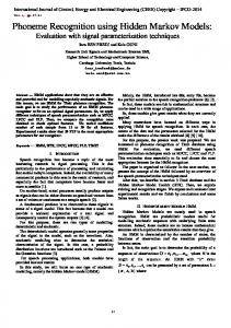
On the other hand, the 2 newly proposed algorithms are much faster than standard gradient descent. From Table 1 and Figure 1, we observe that standard gradient descent, even when an optimal learning rate has been chosen (η = 0.02), requires as much as five times the number of iterations in order to reach the appropriate loglikelihood. We should mention here, that in real life applications, we would have chosen a threshold for the difference in the log-likelihood, between two consecutive iterations (for example 0.01). In such cases the training procedure would have been stopped much earlier, using the two proposed algorithms, than with the standard gradient descent. We should note here, that the observed differences in the values of negative loglikelihood correspond also to better predictive performance of the model. By the use of our two proposed algorithms the correlation coefficient for the correctly predicted residues, in a two state mode (transmembrane vs. non-transmembrane), ranges between 0.848-0.851, whereas for standard gradient descent ranges between 0.8190.846. Similarly, the fraction of the correctly predicted residues in a two state mode ranges between 0.899-0.901, while at the same time the standard gradient descent

50

Pantelis G. Bagos, Theodore D. Liakopoulos, and Stavros J. Hamodrakas

Fig. 1. Evolution of the negative log-likelihoods obtained using the three algorithms, with the same initial values for the learning rate (0.02). This learning rate was found to be the optimal for standard gradient descent. Note that after 50 iterations the lines for the two proposed algorithms are practically indistinguishable, and also that convergence is achieved much faster, compared to standard gradient descent

yields a prediction in the range of 0.871-0.885. In all cases these measures were computed without counting the cases of divergence, where no useful model could be trained. Obviously, the two algorithms perform consistently better, irrespective of the initial values of the parameters. If we used different learning rates for the emission and transition probabilities, we would probably perform a more reliable training for standard gradient descent. Unfortunately, this would result in having to optimize simultaneously two parameters, which it would turn out to require more trials for finding optimal values for each one. Our two proposed algorithms on the other hand, do not depend that much on the initial values, and thus this problem is not present.

5 Conclusions We have presented two simple, yet powerful modifications of the standard gradient descent method for training Hidden Markov Models, with the CML criterion. The approach was based on individually learning rate adaptation, which have been proved useful for speeding up the convergence of multi-layer perceptrons, but up to date no such kind of study have been performed on HMMs. The results obtained from this study are encouraging; our proposed algorithms not only outperform, as one would expect, the standard gradient descent in terms of training speed, but also provide a much more robust training procedure. Furthermore, in all cases the predictive performance is better, as judged from the measures of the per-residue accuracy mentioned earlier. In conclusion, the two algorithms presented here, converge much faster

Faster Gradient Descent Training of Hidden Markov Models

51

to the same value of the negative log-likelihood, and produce better results. Thus, it is clear that they are superior compared to standard gradient descent. Since the required parameter tuning is minimal, without increasing the computational complexity or the memory requirements, our algorithms constitute a potential replacement for the standard gradient descent for CML training.

References 1. Rabiner, L.: A tutorial on hidden Markov models and selected applications in speech recognition. Proc IEEE. 77(2) (1989) 257-286 2. Durbin, R., Eddy, S., Krogh, A., Mithison, G.: Biological sequence analysis, probabilistic models of proteins and nucleic acids. Cambridge University Press (1998) 3. Krogh, A., Larsson, B., von Heijne, G., Sonnhammer, E.L.: Predicting transmembrane protein topology with a hidden Markov model, application to complete genomes. J. Mol. Biol. 305(3) (2001) 567-80 4. Henderson, J., Salzberg, S., Fasman, K.H.: Finding genes in DNA with a hidden Markov model. J. Comput. Biol. 4(2) (1997) 127-142 5. Krogh, A., Mian, I.S., Haussler, D.: A hidden Markov model that finds genes in E. coli DNA. Nucleic Acids Res. 22(22) (1994) 4768-78 6. Baum, L.: An inequality and associated maximization technique in statistical estimation for probalistic functions of Markov processes. Inequalities. 3 (1972) 1-8 7. Dempster, A.P., Laird, N.M., Rubin, D.B.: Maximum likelihood from incomplete data via the EM algorithm. J. Royal Stat. Soc. B. 39 (1977) 1-38 8. Baldi, P., Chauvin, Y.: Smooth On-Line Learning Algorithms for Hidden Markov Models. Neural Comput. 6(2) (1994) 305-316 9. Krogh, A.: Hidden Markov models for labeled sequences, Proceedings of the12th IAPR International Conference on Pattern Recognition (1994) 140-144 10. Krogh, A.: Two methods for improving performance of an HMM and their application for gene finding. Proc Int Conf Intell Syst Mol Biol. 5 (1997) 179-86 11. Bagos, P.G., Liakopoulos, T.D., Hamodrakas, S.J.: Maximum Likelihood and Conditional Maximum Likelihood learning algorithms for Hidden Markov Models with labeled dataApplication to transmembrane protein topology prediction. In Simos, T.E. (ed): Computational Methods in Sciences and Engineering, Proceedings of the International Conference 2003 (ICCMSE 2003), World Scientific Publishing Co. Pte. Ltd. Singapore (2003) 47-55 12. Krogh, A., Riis, S.K.: Hidden neural networks. Neural Comput. 11(2) (1999) 541-63 13. Bishop, C.M.: Neural Networks for Pattern Recognition. Oxford University Press (1998) 14. Schiffmann, W., Joost, M., Werner, R.: Optimization of the Backpropagation Algorithm for Training Multi-Layer Perceptrons. Technical report (1994) University of Koblenz, Institute of Physics. 15. Riedmiller, M., Braun, H.: RPROP-A Fast Adaptive Learning Algorithm, Proceedings of the 1992 International Symposium on Computer and Information Sciences, Antalya, Turkey, (1992) 279-285 16. Schulz, G.E.: The structure of bacterial outer membrane proteins, Biochim. Biophys. Acta., 1565(2) (2002) 308-17 17. Von Heijne, G.: Recent advances in the understanding of membrane protein assembly and function. Quart. Rev. Biophys., 32(4) (1999) 285-307

52

Pantelis G. Bagos, Theodore D. Liakopoulos, and Stavros J. Hamodrakas

18. Bagos, P.G., Liakopoulos, T.D., Spyropoulos, I.C., Hamodrakas, S.J.: A Hidden Markov Model capable of predicting and discriminating β-barrel outer membrane proteins. BMC Bioinformatics 5:29 (2004) 19. Moller S., Croning M.D., Apweiler R.: Evaluation of methods for the prediction of membrane spanning regions. Bioinformatics, 17(7) (2001) 646-53 20. Bagos, P.G., Liakopoulos, T.D., Spyropoulos, I.C., Hamodrakas, S.J.: PRED-TMBB: a web server for predicting the topology of beta-barrel outer membrane proteins. Nucleic Acids Res. 32(Web Server Issue) (2004) W400-W404 21. Berman, H.M., Battistuz, T., Bhat, T.N., Bluhm, W.F., Bourne, P.E., Burkhardt, K., Feng, Z., Gilliland, G.L., Iype, L., Jain, S., et al: The Protein Data Bank. Acta Crystallogr. D Biol. Crystallogr., 58(Pt 6 No 1) (2002) 899-907