Hindawi Publishing Corporation Mobile Information Systems Volume 2015, Article ID 818307, 18 pages http://dx.doi.org/10.1155/2015/818307
Research Article FastFlow: Efficient Scalable Model-Driven Framework for Processing Massive Mobile Stream Data Cang-hong Jin,1,2 Ze-min Liu,1 Ming-hui Wu,2 and Jing Ying1 1
College of Computer Science and Technology, Zhejiang University, Hangzhou 310027, China Department of Computer Science and Engineering, Zhejiang University City College, Hangzhou 310015, China
2
Correspondence should be addressed to Ming-hui Wu;
[email protected] Received 18 January 2015; Revised 15 April 2015; Accepted 28 April 2015 Academic Editor: Laurence T. Yang Copyright © 2015 Cang-hong Jin et al. This is an open access article distributed under the Creative Commons Attribution License, which permits unrestricted use, distribution, and reproduction in any medium, provided the original work is properly cited. Massive stream data mining and computing require dealing with an infinite sequence of data items with low latency. As far as we know, current Stream Processing Engines (SPEs) cannot handle massive stream data efficiently due to their inability of horizontal computation modeling and lack of interactive query. In this paper, we detail the challenges of stream data processing and introduce FastFlow, a model-driven infrastructure. FastFlow differs from other existing SPEs in terms of its user-friendly interface, support of complex operators, heterogeneous outputs, extensible computing model, and real-time deployment. Further, FastFlow includes optimizers to reorganize the execution topology for batch query to reduce resource cost rather than executing each query independently.
1. Introduction and Motivation Tremendous and potentially infinite volumes of data streams are generated by real-time surveillance systems, communication networks, online transaction process, and other dynamic environments [1]. Due to the high commercial and research value of these massive stream data, numerous Stream Processing Engines (SPEs) have been proposed to process those data, from both industry and academic community. Differing in their system architectures, operation models, and/or rule languages, many of these SPEs are converted to notable mature products during the last decade [2] (e.g., StreamBase [3], InfoSphere Streams [4], Storm [5], and Apama [6]). These SPEs may offer very different functionalities because of their diverse purposes and focuses (e.g., stock market analysis, utility studies, process, and quality control), but due to unique characteristics of stream data all of them should meet the common requirements: one-pass scan without persistent storage of the whole stream and processing steam on the fly. Note that traditional DBMS (Database Management System) needs to store and index data before analyzing it and thus cannot fulfill the requirements very well [7].
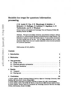
Although there are a number of existing SPEs offering solutions to handle Complex Event Processing (CEP) problem, we argue that two main challenges require better solutions. First, traditional SPEs (e.g., Esper, SQLStream, and StreamBase) are designed to handle medium-sized sequence records. Hence, the computation power of a single server is not enough when the volume of stream data is huge. As Figure 1(a) shows, a common solution for this issue is to use scaling-up strategy that partitions and replicates data to multiple servers. However, this scale-up solution makes it hard to reuse intermediate results because different logics are assigned to separate computing nodes and thus may waste computing resource for redundant computation. Second, lack of interaction during the analytical process reduces the flexibility of these SPEs. For instance, Storm and Apache S4 only supply primitive operations to analysts and use Directed Acyclic Graph (DAG) to schedule execution logic. DAG is a computing model in which each edge terms a stream and each vertex is a primitive operator. Figure 1(b) depicts the DAG model. Using DAG model, business logics should be predefined and translated into machine understandable program by software developers and then deploy to
2
Mobile Information Systems
Sink 1 Rule 1
Sink 2
Sink 1 Sink 2 .. .
Rule n
Rule 2 ···
Stream Shuffle component
Horizontal cluster
Sink n Substream
Stream
Substream Rule i
Sink n
Rule j
Sink i
Sink j
Rule 1, 2, . . . , n
(a)
(b)
Figure 1: Two implementation architectures of handling massive stream data. (a) terms scale-up model, which splits input stream into several substreams by hash function or manually. Analysts define business logic requirements as separated rules that are sent to operator nodes in queue. The relation of source, operator, and sink is (1-1-1), while (b) presents a horizontal distributed computing model, which treats rules as a set and shares stream data among multiple operators. Hence, the relation of source, operator, and sink is (1-n-n).
Table 1: Features of representative stream processing engines. Free or commercial
Computing model
Build business logic online
Rule types
Commercial
Scale-up
Yes
Declarative and SQL-like
Drools Storm Apache S4
Free Free Free
Scale-up Horizontal Horizontal
No No No
Declarative Provide basic primitives Provide a bit more basic primitives than Storm
StreamBase FastFlow
Commercial Prototype
Scale-up Horizontal
Yes Yes
Declarative and SQL-like SQL-like
Esper
the servers. Thus business logics cannot be changed on the fly. Hence, SPE systems like Storm and Apache S4 cannot flexibly adopt customers’ changes on business logics. To overcome these issues exposed by existing SPEs, we aim to propose a solution with efficient resource usage, flexible logic deployment, and easy scale-up. Among various important tasks of SPEs we already mentioned, in this paper we focus on mining the dynamically updated statistical mobile data of a user track system. More specifically, the system collects semistructured stream data flow continuously and incorporates essential data mining techniques such as association and characterization on real time. Since traditional database systems cannot handle these temporally ordered, fast changing, massive, and potentially infinite data [7], here, we present a novel stream data processing framework FastFlow, which consists of web UI model, XML formatted metamodel, and execution model. The unique features of FastFlow include enabling of changing business logic on the fly and better scaling of computing power. We will show that a SQL-user should be able to quickly grasp stream processing with ease. Current Situations and Challenges. We compare features of common SPEs with FastFlow in Table 1. Some engines (e.g., Esper, Drools) support changing rule on the fly but cannot deal with massive data very well due to their scale-up distribution designs [8], while other systems (e.g., Storm, Apache S4) can support easy-extension deployment but only offer primitive operators. In contrast, FastFlow supports both horizontal computing model and flexible logic definition. In this paper, our framework only supports some simple stream
queries and operations, but it can be extended to handle more complex queries and rules. Our Contributions. In this paper, we make the following contributions. First, in FastFlow we supply user-friendly web UI for users to build and deploy business logic model on the fly; that is, FastFlow allows users define and modify business logic without programmers involved. Second, we model the cost of primitive operations and achieve accurate estimation of global cost of given business logic. Third, FastFlow contains optimizers (local optimizer for single query and global optimizer batch query) to effectively reorganize query execution topology to enhance efficiency.
2. Business and Technique Background 2.1. Mobile Stream Data. In this paper, we categorize the features of mobile data into two classes: demographic feature and activity feature. Demographic feature includes static content of mobile device such as device manufacturer (e.g., Samsung, Apple, and Xiaomi), smartphone models (e.g., iPhone 5S, Note 2, and Mi3), OS version (e.g., IOS 7 or Android 4.0), device screen size, CPU, RAM, and device price. Activity features which record mobile events include GPS location, various sensors’ collected data, application list, connected net type, and currently running applications. Hence, activity features present a stream of up-to-the-minute activity across the device which reflects the user behavior [9].
Mobile Information Systems
3 Big data processing model
Real-time model
Interactive model
Online system Real-time analytics Complex event processing
Parameterized report OLAP Visualization exploration
Esper, Storm, and Yahoo S4
Impala, Shark, and Presto
Noninteractive model
Batch model
Data preprocessing Incremental batch processing Dashboard Hadoop, Sqoop
Data mining Daily enterprise report Batch processing Hadoop, Tez, Stinger, Disco, and HPCC
Figure 2: A hierarchical architecture of big data processing models, covering batch and real-time categories, including real-time model, interactive model, noninteractive model, and batch model.
2.2. Data Collection and Storage. In SPEs once a stream data item is processed, it is usually discarded and cannot be reoperated since SPEs do not have enough space to store archive data. FastFlow works under the same requirement. In the context of mobile stream data, once the application status changed, SDK would generate an event record and upload to collection server. Millions of application events produce a huge amount of data streams continuously. Before sending data to FastFlow, we do dictionary coding and duplication removing in some distributed memory storage systems as Redis [10] and Kafka [11]. 2.3. Data Processing Models. As Figure 2 shows, commercial and mature big data platform can be generalized as four different models: real-time model, interactive model, noninteractive model, and batch model. Real-Time Processing Model. Real-time data processing model (RTM) involves continuous stream data, online processing, and output report. RTM systems process diverse data sources with very small latency and are applied in bank ATMs and customer service system. Some RTM systems like Esper, Storm, and S4 have been well developed in recent years. Interactive Model. Like DBMS in traditional industry, interactive model (IM) is designed for parameter-based querying and multiple points visualization exploring. In terms of big data operation, IM platform accepts user command input and executes command in computing environment. Cloudera Impala, Databricks Shark, and Presto are such examples of IM systems. Noninteractive Model. Unlike interactive model which needs human operation, noninteractive model (NIM) systems run with relative fixed process logic. Therefore, NIM is usually used as data preprocessing or data extract, transform, and load (ETL) tool. For example, Hadoop and Sqoop could be treated as ETL tools to migrate data from relational database to Hadoop Distributed File System (HDFS). Batch Model. Batch model (BM) is suitable for those tasks that have long running process without manual intervention.
Data are preselected and commands are predefined in scripts; BM programs process jobs without human interaction. BM systems, such as Hadoop, Tez, Stinger, Disco, and HPCC, have the benefit of allowing users to log out system or disconnect without stopping the running jobs. Based on four different models above, FastFlow falls into a mixed model of real-time and interactive ones. Similar to what Impala and DBMS do, FastFlow supports SQLlike query model and processes stream data in real time. Furthermore, FastFlow does not need to index and store stream data in files like other DBMSs do, and it could return continuous result as CEPs do. 2.4. Model Driven Architecture on Big Data. Model Driven Architecture (MDA) is used to describe the concepts and their relations for system framework [12]. A system can be expressed by an abstraction model at different levels where each level presents certain aspects of the system. Object Management Group (OMG) [13] defines three different models of MDA: concept model, metamodel, and platform model. Concept model has the highest abstraction and is described in business viewpoint. Metamodel is platform independence level with technological viewpoint. Platform model gives the most detailed information of system implementation and generates execution code for various running environments. MDA promotes the creation of machine-readable, highly abstract models that are developed independently of implementation technology. Several MDA related approaches are proposed for migrating system from traditional platform to cloud platform [9]. Article [14] proposes a model-driven tool for analyzing real-time stream processing applications so that performance bottlenecks can be pinpointed. The idea and mechanism of MDA are introduced in our paper. FastFlow accepts concept model by web UI, transforms model to metamodel with optimizers, and finally implements model on special storm platform.
3. Model-Driven FastFlow Framework In this section, we give the overview of FastFlow. Following the model-driven architecture in Figure 3, we define all three
4
Mobile Information Systems
Concept model
0···1
Metamodel
Instance of
1···n 0···1
Platform
Transformation
Figure 3: Model Driven Architecture transformation process.
OperatorNode Sessions
Events
Devices Events Stream data
From(events) Source chosen
Events Where(model = samsung) 𝜎 operator
Select(userid) Π operator
Linear order
Figure 4: Split query into a set of operators and organize in linear order.
main component models (concept query model, operation node model, and topology model) which are related to the three abstraction levels accordingly. 3.1. Interactive Concept Model Definition. Unlike other SEPs which require developers’ involvement in implementation of business logic, FastFlow offers a web interface to human agents without knowing much technical details of the system to easily define business logic. For example, one can simply issue a query “select nettype, region, model from events where nettype = ‘Wi-Fi’ [Range 10 min]” to extract phone model and related areas for those Wi-Fi users in the past ten minutes. 3.2. Modularize Metamodel via Composite Operators. When a user defines and submits the concept model via GUI, the concept model needs to be transformed to a set of basic fundamental operators. We provide three major operators in FastFlow. OperatorNode. OperatorNode (ON) is a computing element in FastFlow and is categorized into three classes by its sources and sinks: monadic operator model, combine operator model, and separate operator model. ON is determined by the number of input streams and output streams. Monadic operator model works for the cases with single input stream and single output stream. Monadic operator includes select node, where node, rename node, aggregate node, and arithmetic nodes. Combine operator accepts multiple data stream as input, processes them, and outputs single output stream. For instance, join node and union node are combine operators. Separate operator has single stream source as input and copies or shuffles it to several successors. TimeNode. TimeNode (TN) in FastFlow defines the sliding time window for executing query model and manages finegrained event expiry. TN informs the engine how long each relevant query task should be retained and also improves the efficiency of cluster resource by discarding expired tasks. CacheNode. The main purpose of CacheNode (CN) is to temporarily save data in local or distributed storage. Since
some operators are aggregation based and ranking based (e.g., sum, count, and top-𝑘), CN saves and updates current event status tentatively and can be treated as a connection node among different ONs. Operator nodes and their relations can be described as CM(𝑁, 𝑅), where 𝑁 is OperatorNode, TimeNode, or CacheNode (i.e., select, where, and from) and 𝑅 could be presented as an arrow from one node to its successor like 𝑅(𝑛start , 𝑛end ). For example, a query “select userid from events where model = ‘Samsung”’ consists of three OperatorNodes: select (userid), from (events), and where (model = “Samsung”). Select, from, and where are operators while objects in brackets are attribute items. One possible implementation of query is expressed in Figure 4, in which all three operators are linearly ordered. When a tuple of stream data comes, it will be processed through the first node to the last node. Beside the above three main basic operators, we present a directed acyclic graph (DAG), formed by a set of vertices and edges, to model business logic in partial orders. A vertex presents a single operator and an edge shows constraint. DAGs could be used to generate processes in which data flows in a consistent direction through a network of processors. Besides taking operator functions into account, in our framework, we also consider the intermediate results reuse in DAG to reduce the cost of cluster resources. 3.3. Metamodel Structure and Persistence. Metamodel could be defined by source, operator, and sink. In addition, we also give a description of cluster environment like number of nodes in cluster, the parallelism of node, and the throughput of sources and sinks. We choose Extensible Markup Language (XML) as our persistence model, which is structureformatted and easy to define business semantic by holders. A variety of XML tools and API have been developed and rich online documents and examples are easily to touch. Since metamodel is not platform dependent, it can exchange and transfer model to multiple platforms prevalently [15]. In FastFlow, we describe metamodel in three folders: running environment, data structure description, and execution topology. Algorithm 1 shows the structure of metamodel in XML.
Mobile Information Systems
5
300000 cluster sid app id usr id sess stamp sess zone ⋅⋅⋅ ⋅⋅⋅ 2 WWIIFrontline ⋅⋅⋅ Algorithm 1: XML formatted metamodel with three submodules, including system configuration, data format, and operator description.
We use the element “configuration” to denote the feature of processing cluster. Element “executionTime’’ defines the range of sliding window, that is, 30000 ms, while “executionType” terms cluster or local mode to execute topology. Element “dataFormat” gives schema of stream data including data source connection information, data type, and attribute name. Finally, “operators” describes function type, storm grouping type, and operating parameter condition. 3.4. FastFlow Processing via MDA. According to the components in MDA model, the overview of FastFlow framework processing includes four parts in Figure 5: user-friendly web UI, FastFlow engine, cluster environment, and data source. Business analysts describe logic via web UI. Then the logic is transferred to metamodel. FastFlow engine accepts metamodel and parses it into operator nodes, applies optimizers to reorganize execution topology, and generates machine understandable execution code. The execution code is distributed to cloud cluster. Once the code is executed on the cluster, outputs are extracted continuously. Note that the local optimizer and the global optimizer included in FastFlow engine are designed to generate optimal execution topology.
4. Operator Cost Estimation and Optimization In this section we focus on how to transfer metamodel to execution plan efficiently. We introduce how to measure resource cost for different operators and give two optimizers to improve efficiency of resource utility.
4.1. Estimate Costs of Operators. Since user cannot access model transformation functions directly, we need an optimizer to accept metamodel, parse model, and find the best execution plan. For those data streaming environment with multiple nodes in scalable cluster like Storm or S4, data processing plan is treated as DAG and allocated to several connected nodes. The primary resources in cluster are available CPUs, memory, and network bandwidth. Hence, our optimizers aim to optimize the utility of these resources. There are still two challenges left for optimizing plan. One is how to weight resource because a variety of applications are running in heterogeneous clusters. Different application administrators focus on different facets according to their available resources. For example, when the cluster is short of CPU, the efficiency of algorithm has more weight than I/O performance. In this paper, the term 𝑆𝑇 is defined as resource of type 𝑇. For example, we can present 𝑆CPU as CPU resource. Instead of treating importance of all resources equally, we give a special value for every type of resources by 𝑊𝑇 . Moreover, for distributed cluster systems, if we want to monitor the utility of certain computing node, the term could be presented as 𝑤𝑟op , where 𝑟 is resource type and op is computing node. Another challenge is how to predict resource cost for different implementations. We introduce statistic-based approaches to estimate resources cost. Suppose that tuple in stream data has 𝑛 attributes with type int, vchar, and so forth, we give naive estimation model and complex estimation model to predict field size (PFS) for projection operation (i.e., select). For naive estimation model, we only consider the number of attributes in tuples regardless
6
Mobile Information Systems Various outputs Get continuous result
Generate continuous data
FastFlow core engine Local optimizer FastFlow core engine
Topology and execution code
Choose report type
Define concept model
Clusters Kafka or Redis
Stream data source
Analysts
Select data source
Operator nodes
Rule repository
Transformation engine
Global optimizer
Metamodel WebUI
Figure 5: Overview of processing by FastFlow. It can be organized into three phases, including web-based business concept model definition, FastFlow core engine, horizontal scalability cluster, and various perspectives.
of attribute type. For example, given an 𝑛-attribute tuple, PFS for 𝑘 selected field is 𝑘/𝑛, while for complex estimation model, PFS takes filed type into account and defines formula as PFS(attr𝑘 ) = FiledSize(attr𝑘 )/ ∑𝑛𝑖=1 FiledSize(attr𝑖 ). Furthermore, selection operations (i.e., where) can filter small parts of whole records and discard others. Therefore, the selectivity of a condition 𝜃𝑖 is the probability that a tuple in the source 𝑟 satisfies 𝜃𝑖 . If 𝑠𝑖 is the number of satisfying tuples in 𝑟, the percentage of selected size (PSS) is 𝑠𝑖 /𝑛𝑟 . For a set of conjunction selection operations 𝜃1 , 𝜃2 , . . . , 𝜃𝑘 , the estimate cost is given by formula PSS (𝜎𝜃1∧𝜃2⋅⋅⋅∧𝜃𝑘 (DS)) = 𝑠1 × 𝑠2 × ⋅ ⋅ ⋅ × 𝑠𝑘 /𝑛𝑟𝑘 . Similarly, the disjunction and negation estimations are PSS (𝜎𝜃1∨𝜃2⋅⋅⋅∨𝜃𝑘 (DS)) = 1 − (1 − 𝑠1 /𝑛𝑟 ) × (1 − 𝑠2 /𝑛𝑟 ) × ⋅ ⋅ ⋅ × (1 − 𝑠𝑛 /𝑛𝑟 ) and PSS(𝜎¬𝜃𝑖 (DS)) = 1 − 𝑠𝑖 /𝑛𝑟 . We treat reduction factor 𝑟𝑓op as PFS or PSS for special operator op and estimate global resource cost by formula gc = ∑op∈⟨ops⟩ ∑ 𝑟∈⟨CPU,mem,bandwidth⟩ 𝑟𝑓op × 𝑤𝑟op . If the topology has smaller gc, it has more efficient resource usage in high probability. 4.2. Equivalence Rule Optimization. In order to optimize the execution topology, we should have some criteria to guarantee the function semantic stable during various implementations. Equivalence rule defines the situation of several execution processors that if we give the same inputs any processors then we would get the same result. For example, in query “select userid from events where model = ‘samsung’,” from (events) model points out that data source and others operators describe projection and filter functions. We could see that execution paradigms “from-select-where” and “fromwhere-select” would have the same outputs and meet equivalence rules. In this paper, we focus on single stream source with multiple queries for simple and define five equivalence rules, including the following. ER1 (equivalent conjunctive selection). Conjunctive selection operation could be reconstructed into a sequence of separated
selections as 𝜎𝜃1∧𝜃2 (DS) = 𝜎𝜃1 (𝜎𝜃2 (DS)), where DS is data source and 𝜃 is selection condition. ER2 (equivalent commutative selection). The selection operations can switch position like 𝜎𝜃1 (𝜎𝜃2 (DS)) = 𝜎𝜃2 (𝜎𝜃1 (DS)). ER3 (equivalent multiple projections). Only the last projection operation is needed while others could be ignored as ∏𝑡1 (∏𝑡2 (⋅ ⋅ ⋅ (∏𝑡𝑛 (DS)) ⋅ ⋅ ⋅ )) = ∏𝑡1 (DS), where 𝑡𝑖 denotes a project attribute. ER4 (equivalent sliding window). The sliding window could be added to any function operation. For example, 𝜎𝜃1∧𝜃2 (DS)[Range], 𝜎𝜃1 (𝜎𝜃2 (DS[Range])), and 𝜎𝜃1 (𝜎𝜃2 (DS)[Range]) are the same, where Range denotes the slidingwindow size. ER5 (equivalent exchange). Projection operation and filter operation could be exchanged in linear order as ∏𝑡 𝜎𝜃 (DS) = 𝜎𝜃 ∏𝑡 (DS). The above five rules will be used in query transform process and be designed for reducing resource cost via alternative implementations. The similar idea could be found in traditional query optimizer [16]; however in this paper these rules do not only focus on single query processing but also intend to optimize multiple queries in cluster nodes. 4.3. Topology Optimization Design. FastFlow includes two kinds of optimizers, Local optimizer and Global optimizer, to deal with resources allocation at different levels. Local optimizer, which focuses on single query, reorganizes execution topology to reduce resources cost. Global optimizer tries to optimize the overall efficiency of multiple tasks, for example, by reusing the intermediate results across different tasks. By using equivalent rules, we could translate business logic to multiple metamodels and estimate resource cost of
Mobile Information Systems
7
Input: : operation model list 𝑐op : cost of cpu, memory and network for special operators 𝑤𝑟op : weight for resource and operator Output: metaModel: the optimal execution way (1) Initialize (0-1)-matrix operatorMatrix(𝑜𝑝𝑀1 , 𝑜𝑝𝑀2 ) (2) metaModel ← (3) metaModel ← opMsliding window (4) vertex ← 0, minweight ← 0 (5) for all opM in operationModel do (6) if opM.type = source selection then (7) metaModel ← opMsource (8) operationModel\opMsource (9) else (10) vertex ← opMsource (11) for all opM in operationModel do (12) if operatorMatrix(vertex, opM) = 1 and min{𝑐𝑜𝑝𝑀 , 𝑚𝑖𝑛𝑤𝑒𝑖𝑔ℎ𝑡} < 𝑚𝑖𝑛𝑤𝑒𝑖𝑔ℎ𝑡 then (13) vertex ← opM and operationModel\opM and metaModel ← opM (14) 𝑚𝑖𝑛𝑤𝑒𝑖𝑔ℎ𝑡 ← min{𝑐𝑜𝑝𝑀 , 𝑚𝑖𝑛𝑤𝑒𝑖𝑔ℎ𝑡} (15) else (16) continue (17) end for (18) end if (19) end for (20) return metaModel Algorithm 2: Local optimizer.
each model. In this section, we present the algorithms of local optimizer and global optimizer. 4.3.1. Local Optimizer. Local optimizer is responsible for generating optimal execution plan for single query task. As described in Figure 4, a single task could be expressed as a linear sequence with special order. Algorithm 2 is a method to estimate cost for given strategy and find the optimal way to implement business logic. In Algorithm 2, we denote operators of each query as a set of tuples . We first generate operatorMatrix, a (0, 1)-matrix according to equivalent rules, to express the connection of two operators. The sliding-window operator and source operator are put at the beginning (i.e., lines 3–10). For other operators, we connect them by taking both equivalent rules and estimated resource cost into consideration. We evaluate cost for each operator and put smaller cost node in the front (i.e., lines 11–19) such that most parts of data could be discarded earlier to release the resource. 4.3.2. Global Optimizer. Global optimizer focuses on cluster performance by multiple queries. For each data stream, there are many queries for different business logic, which could be clustered to multiple sets by their operators. Queries in special set are more similar than queries outside. For instance, there are four query models Q1, Q2, Q3, and Q4 in a cluster, which are expressed in Box 1. According to operator nodes, these queries have common parts shared among each other (like select region or where nettype = “Wi-Fi”). For those queries, unlike traditional DBMS (MySQL, PostregSQL) and scale-up CEPs (drools, Esper) to treat
opj
opi
Sequence
opi
opj
opj
···
···
opk
opk
AND split
opi
AND join
Figure 6: Define basic connection model in DAG based on their source and sink, including sequence, AND split, and AND join.
queries independent and handle them separately, FastFlow integrates multiple execution paths and generates a global execution topology. We show three basic topology connection types in Figure 6: sequence, AND split, and AND join. Sequence supports both single query and multiple queries. AND split and AND join are suitable for merging multiple queries. Any topology with complex logic could be composed by these three basic models. We present the global optimizer in Algorithm 3 which consists of four separate steps: extracting common operators, evaluating similarity of queries, local optimizer, and global optimizer. We use Figure 7 to illustrate process of global optimizer. First, we extract common operators, which are shared in more than one query, from simple to complex models, categorize operators into three folders, and mark operator code from one to six. Then, we use Jaccard similarity coefficient [17], a
8
Mobile Information Systems
Q1: select nettype, region, model from events where nettype = “Wi-Fi” [Range 10 min] Q2: select nettype, region, model, user, receivetime, ip from events where nettype = “Wi-Fi” [Range 10 min] Q3: select nettype, region, model, user, receivetime, ip from events where nettype = “Wi-Fi” and ip contains “117.136” [Range 10 min] Q4: selectdistinct(user) from events where nettype = “Wi-Fi” [Range 10 min] Box 1: Four queries in certain cluster with high relativity.
Input: : a set of operation list 𝑐op : cost of cpu, memory and bandwidth for special operation 𝑤𝑡 : weight of different resources Output: metaTopology: the optimal execution topology Step 1. Initialize and split basic operators (1) Initialize (0-1)-matrix OperationMatrix(𝑜𝑝𝑀1 , 𝑜𝑝𝑀2 ) (2) Extract basic operators com(operationModel) from Step 2. Set similarity of multiple queries (3) calculate pairwise JaccardSimilarity(Q1, Q2) (4) ← order pairwise queries by their similarity score Step 3. Local optimizer (5) localoptimalTopology ← (6) localoptimalTopology ← Meta-Model Local Optimize(, cop , 𝑤𝑡 ) Step 4. Global optimizer (7) metaTopology ← (8) for all Q1, Q2 in do (9) if Q1, Q2 not in metaTopology then (10) metaTopology ← Merge Q1, Q2 and keep global semantic (11) end for (12) return metaTopology Algorithm 3: Global optimizer.
statistic method for comparing the similarity of different sets, to calculate the score of pairwise queries. Jaccard similarity (JS) could be expressed as formula JS(𝐴, 𝐵) = |𝐴 ∩ 𝐵|/|𝐴 ∪ 𝐵|, where 𝐴 and 𝐵 are two sets. As Figure 7 shows, set Q1 has code (1, 5) and Q2 has code (1, 2, 3, 5); thus the Jaccard similarity JS(Q1, Q2) = 0.5. We list all similarity scores for six pairwise queries in Steps 1-2. Next, Step 3 plans resource-cost optimal execution path for every query by Algorithm 2. In Step 4, we merge local optimal queries by the descending order of their similarity score. Note that execution order in global optimizer might be different with the order in local optimizer because we need to keep the query semantic for all queries in global topology. For example, in order to merge Q2 and Q3, filter operator (code 4) should be moved from the beginning node to the end node. Q1 changes the order of execution path as well for matching existing topology completely.
5. FastFlow Implementation According to the three phases in the MDA architecture, the concept model is defined by queries, while the platform-independent model (metaexecution plan) is proposed by optimizers and is stored in structured format files
as XML. Now, we focus on the last phase: how to implement execution plan to specific platform running code. Since Apache Storm is a free and open source distributed real-time computation system. It could be used for real-time analytics, online machine learning, continuous computing, and ETL. Moreover, it is scalable, fault-tolerant, and easy to operate and extend. In this work, we use Storm to set up FastFlow. Figure 8 shows the class design of the FastFlow framework. Some classes inherit from Storm interface. FastFlow contains three main execution components which are also defined in Storm: ISpout, IBolt, and Execution Topology. ISpout defines the input source of system, IBolt processes stream data step by step, and Execution Topology describes global running plan for multiple given tasks. IBolt could be implemented by various operation types like monadic operator, combine operator, and separate operator. To clarify, TaskMetaModel is related to metadata model defined in XML configuration file. Kafka component is treated as storage node. The two optimizers are cooperated with Execution Topology. All the generated codes are deployed to Storm environment for horizontal scale.
Mobile Information Systems
9 Common operators
Code
nettype, region, model receivetime, and ip
Type
Projection
Filter
Query
Similarity
1
Q1
Q2
0.5
2
Q1
Q3
0.4
user
3
Q1
Q4
0.25
Contains “117.136”
4
Q2
Q3
0.8
nettype = “Wi-Fi”
5
Q2
Q4
0.4
distinct(user)
6
Q3
Q4
0.33
Advanced operator
Query
1
1
1
2
5
5
5
4
2
3 (a) Query Q1
(b) Query Q2
1 (Q1, Q2, Q3)
2 (Q2, Q3)
4
5
(Q3)
Step 3
6
5
(d) Query Q4
(c) Query Q3
1 5
3
3
(Q2, Q3)
(Q2, Q3)
Steps 1-2
1 (Q1, Q2, Q3)
2
4
(Q2, Q3)
(Q1, Q2, Q3)
5
(Q3)
2
(Q1, Q2, Q3, Q4)
Step 4
4 (Q3)
(Q2, Q3)
3
3
3
(Q2, Q3)
(Q2, Q3)
(Q2, Q3, Q4)
Sim(Q2, Q3) = 0.8
Sim(Q1, Q2) = 0.5
Sim(Q3, Q4) = 0.33
6 (Q4)
Figure 7: A case study of global optimizer. Given four queries, get common operators and calculate query Jaccard similarity in Steps 1-2, generate local optimal execution plan for single query, and merge multiple queries by global optimizer. TopologyBuilder
StormSubmitter + submitTopology()
ExecutionTopology
≪interface≫ IRichBolt + execute()
+ setSpout() + setBolt()
MonadicOperator
CombineOperator
SeparateOperator
- sources - sinks
- sources - sinks
- sources - sinks
+ execute()
+ execute()
+ execute()
+ optimize(): ExecutionTopology
LocalOptimizer
GlobalOptimizer
+ optimize(): ExecutionTopology
+ optimize(): ExecutionTopology
DescribeSpec MetaDataTransform
TaskMetaModel
- metainstance + transform()
XMLParser
StreamBean
ExecutionModel
- operatorModel - executionModel - streamData + generateCode()
OperatorModel 1..*
Optimizer
≪interface≫ IRichSpout + nextTuple()
Kafka
ReadSpout
BIReport
- sources
- type
+ nextTuple()
+ showRpt()
Figure 8: Classes graph of FastFlow main components.
10
Mobile Information Systems 120
320
110
300 280
90
Memory size (MB)
CPU utilization (%)
100
80 70 60
240 220 200
50
180
40 30
260
P(5)
P(10)
P(20) P(30) Size of projection
P(40)
P(50)
160
P(5)
P(10)
P(20) P(30) Size of projection
P(40)
P(50)
3.5
Output bandwidth (MB)
3.0 2.5 2.0 1.5 1.0 0.5
P(5)
P(10)
P(20) P(30) Size of projection
P(40)
P(50)
Figure 9: Resource cost for projection operator. Choose various sizes of projection and estimate CPU utilization, memory usage, and output bandwidth.
6. Performance Evaluation 6.1. Experimental Conditions Platforms. The FastFlow is set up on four-machine cluster, which installs CentOS 6.3 and JDK 7. The cluster includes Dell servers with 8 core Intel Xeon 2.27 GHz, 6TB-size hard disk and interconnected by 1 Gbs network. The RAM of servers is 63.0 GB. The version of Storm is 0.9.0.1. We build web queries interface by PhP and JQuery and use data-driven documents (D3) [18] to output results. Resource Monitor. In order to monitor resource cost of processes in FastFlow, we introduce the Atop tool, an ASCII fullscreen performance monitor, which reports process related resources like CPU utilization, memory consumption, and network throughout. Atops are installed on all cluster servers with a program running to collect machine report every second for further analysis. Note that Storm project cannot support resource monitoring for spout and bolt. In order to track resource of every bolt, we set multiple forts for different Storm workers and
control the number of executors. Then, we could get worker status by its process id. In order to make the experiment nondiscriminatory, we utilize multiple complex operators and run FastFlow for one minute. Dataset. The stream data in our experiment is collected by embedded SDK in mobile applications, which presents user session status information. Each tuple contains 55 fields: 6 string fields (e.g., session), 4 long fields (e.g., applicationId), 8 byte fields (e.g., MAC and IP), and 37 Integer fields (e.g., factoryId, model id). 6.2. Estimate Primitive Operator Performance and Resource Weight. We first analyze the overhead of primitive operator separately on a single server. We choose several common operators, like select, where, distinct, and groupby, to evaluate resource cost like CPU, memory, and network bandwidth. The resource monitor collects 60 tuples and the cost results are presented in Figures 9–11. In these figures, 𝑃(𝑛) means selecting 𝑛 fields to project in query and 𝐹(𝑛) presents choosing 𝑛 where conditions in our experiments.
Mobile Information Systems
11 2.5 Average bandwidth (MB/s)
Average bandwidth (MB/s)
3.5
3.0 2.5 2.0 1.5 1.0 0.5
0
10
P(10) P(20) P(30)
20
30 Runtime (s)
40
50
2.0 1.5 1.0 0.5 0.0
60
0
P(40) P(50)
10
20
30 Runtime (s)
40
50
60
F(3) F(4)
F(1) F(2)
Figure 10: Bandwidth cost for projection operator and filter operator. CPU influence
160
320
140
300 Size of memory (MB)
CPU utilization (%)
120 100 80 60
280 260 240 220
40 20
Memory influence
340
200
Regex
Group Distinct Operator type
Filter(2)
180
Regex
Group Distinct Operator type
Filter(2)
Figure 11: Comparison of resource cost for basic and complex operator types.
In Figure 9, under throughput 2000 tuples per second, with increasing the size of projection, we notice that CPU utilization stays around 70% and memory utilization is around 240 MB. It is obvious that CPU and memory have less influence by projection. However, the output is heavily related to the complexity of projection. The more attributes extracted, the larger output bandwidth needed. Figure 10 shows the result of bandwidth cost for different filter conditions projection operators. We can observe that the decrease in efficiency of filter operator (e.g., where) is usually smaller than projection operator (e.g., select). Because filter operators prune tuples based on the distribution of data value, projection operators prune data by fixed structures and thus when merging an additional condition, the conjunction set size will decrease rapidly. For those advanced operators
(i.e., grouping, regex rule, and distinct), we monitor their CPU and memory utilization in Figure 11. We find that the group operator is the most costly since it has to apply hash function on each item for allocation. The experiments above estimate the resource cost of various operator types. Now we show the influence of stream data throughput. We vary steam data emitting ratio from 2000/second to 20000/second and present results in Figure 12. We can see that CPU usage increases with bigger the throughput, but memory usage is not affected much by varying throughput. In order to set the resource weights of CPU, memory, and bandwidth, we should take into consideration both the above analytical experiments and the limitation of these resources in our cluster. We can draw the conclusion that
Mobile Information Systems 300
500
250
450
Size of memory (MB)
CPU utilization (%)
12
200 150 100 50 0 2000 4000 6000 8000 10000 12000 14000 16000 18000 20000 Throughput Projection Distinct
Regex Filter
400 350 300 250 200 150 2000 4000 6000 8000 10000 12000 14000 16000 18000 20000 Throughput Regex Filter
Projection Distinct
Figure 12: CPU and memory cost for different operator types under increasing throughput.
Table 2: Resource weight of various operators in our experiment.
Projection filter Advanced Ops
CPU 0.5 0.4 0.3
Memory 0.1 0.05 0.1
Bandwidth 0.3 0.4 0.2
CPU and bandwidth are relatively more sensitive to operator type and data volume while memory usage is relatively stable. We further argue that the limitation of hardware resource, maximum of CPU, memory, and bandwidth are 800%, 63 GB, and 100 MB. From Figures 9–12, CPU usage is around 10– 20%, memory is nearly 0.5%, and bandwidth is around 2%. It does make sense for stream data processor since the tuples do not need to be stored (i.e., need not large RAM) and should be handled on the fly (i.e., CPU is busy). According to the resource occupation percent above, we set the related weights for various operators. Setting value to tuple is flexible. In real application, weights could be predefined by suitable rules or adjusted online by cluster current status. Table 2 shows the fixed value for our following experiments by using self-defined formula 𝑝 𝑤𝑅 = (slop + percent) × 𝑚, where slop factor is used for data size increase impaction and 𝑚 is fixed to magnify final value. 6.3. Local Optimizer Performance. In this section, we report the performance of local optimizer. We also compare its effectiveness with normal execution model. Since the initial input stream and final output results are the same no matter which execution plan is used, we only focus on the internal bandwidth between operators. Taking Q 1–3 in Table 1 as examples and following the process in Figure 7, we could estimate the priorities of different queries and different execution plans. Recall that there are two cost-based estimated models: na¨ıve model and complex model. For na¨ıve estimation, in our experiment, there are a total of 55 fields in each tuple with equal weight, while for complex estimation, the field type and definition should be considered. We calculate the cost of filed in Q1–3 as follows: nettype = 0.016, region = 0.016,
model = 0.016, user = 0.052, receiveTime = 0.052, and ip = 0.082. We also give the distribution of data values, which could be collected by sample data. In our cases, the cost of “nettype = Wi-Fi” is 0.21 and the cost of “ip contains 117.136” is 0.14. For each query, we give two plan paths and evaluate score by both estimation models. Note that we use local optimizer to generate execution plan 1 but not for plan 2 (i.e., its query order is not changed). In Table 3, we first run queries Q1–3 by two different strategies and treat execution plan 1 as optimal strategy and execution plan 2 as baseline strategy. For both execution plans, we apply na¨ıve model and complex model to estimate resource cost. We find that the choices of optimal plan under different estimation methods are not always the same. In Table 3, the na¨ıve model chooses plan 2 as the optimal one which is not correct for actual evaluation. Hence, the complex model is more accurate than na¨ıve model, especially when the field types are diverse. Figure 13 presents the resource cost of three types for Q1, Q2, and Q3. It shows that the optimal execution plan delivers significantly better performance. 6.4. Global Optimizer Performance. In order to estimate effectiveness of global optimizer, we first do experiments in Q1–Q4 with two open source tools: Esper and Drools which are used in Twitter and JBoss. These two tools are bestof-breed rule engines which also offer CEP and are easily integrated with java program. We install Esper and Drools rule engine in Storm topology separately, rewrite Q1–Q4 to their special language, and monitor CPU, memory, and bandwidth for one minute under the emit ratio 2000/second. From the results in Figure 14, the CPU utilization of Esper is higher than Drools. However, Drools uses more memory than Esper since it needs additional working memory to store temporary results. In terms of network, the input stream is copied and assigned to different rule engines for both models. Thus, the bandwidth utilizations from two systems are close for all queries. For FastFlow, we set up execution topology with six atom operators as Figure 7 shows and evaluate the recourse cost of them. In Figure 15, we note that resource costs of operators are not balanced, which are highly related to its function as
Mobile Information Systems
13
Table 3: Query execution plan and related priority scores of different models (the weights of operators are in Box 1). Execution Plan 1 (optimal) Na¨ıve estimation Complex estimation 1.24 1.29 0.71 0.66 1.00 0.99
CPU influence
100
Plan path 5-1 (1, 2, 3)-5 (1, 2, 3)-5-4
Execution Plan 2 (normal) Na¨ıve estimation Complex estimation 0.72 0.73 0.93 0.60 0.93 0.59
Memory influence
800 700
80
Size of memory (MB)
600
60
40
500 400 300 200
20
100 0
Q1
Q2
0
Q3
Q1
Q2
Q3
Network influence
800 700 600 Size of bandwidth (MB)
Q1 Q2 Q3
Plan path 1-5 5-(1, 2, 3) 4-5-(1, 2, 3)
CPU utilization (%)
Query
500 400 300 200 100 0
Q1
Q2
Q3
Execution plan 2 Execution plan 1
Figure 13: Comparison of resource cost between normal execution plan and optimal execution plan.
14
Mobile Information Systems CPU influence
70
700
60
600
50 40 30
500 400 300
20
200
10
100
0
Q1
Q2
Memory influence
800
Size of memory (MB)
CPU utilization (%)
80
Q3
0
Q4
Q1
Q2
Q3
Q4
Network influence
1.8
1.6
Size of bandwidth (MB)
1.4 1.2 1.0 0.8 0.6 0.4 0.2 0.0
Q1
Q2
Q3
Q4
Esper Drools
Figure 14: Estimate resource cost of Esper and Drools.
well as its position in topology. For example, operator 5 needs more CPU and bandwidth than others because it needs to handle full dataset which is much bigger than other operators. In contrast, operator 4 is at the end of topology and only deals with only small part of data. Thus these factors should be considered to assign operators to proper machines. At last we compare FastFlow with Esper and Drools on different execution topologies. Based on Figure 7, we evaluate cost for two goals: (1) verify the performance and effectiveness of FastFlow and (2) test the influence of topology structure. The cost of Esper and Drools are the sum of costs of four queries in Figure 14 and the cost of FastFlow
is the sum of resource costs on related operator nodes in Figure 15. As Figure 16 shows, FastFlow has better resource utility than Esper and Drools in all three dimensions, especially in Step 1 and Step 2 where the topologies are the same which means that the additional query does not bring any burden to the whole system.
7. Related Work Our work relates to various past efforts in scalable distributed computation, complex event processing, and MDA.
Mobile Information Systems
15 CPU influence
40
35
300 250 Size of memory (MB)
CPU utilization (%)
30 25 20 15
200 150 100
10
50
10 0
Memory influence
350
op1
op2
op3
op4
op5
0
op6
op1
op2
op3
op4
op5
op6
Network influence
1.8
1.6
Size of bandwidth (MB)
1.4 1.2 1.0 0.8 0.6 0.4 0.2 0.0
op1
op2
op3
op4
op5
op6
Figure 15: Estimate resource cost for all operator nodes.
Large Scalable Computing. Iterative computing models exist in data mining, information retrieval, and other computingintensive applications. For example, MapReduce and Dryad are two popular platforms to take dataflow by a directed acyclic graph operators [7]. HaLoop modifies MapReduce model and supports iterative algorithms [15] and Hone, a “scaling-down” Hadoop, designs a novel mechanism to run program in single multicore high end sever [19]. Projects over MapReduce like Apache Pig and Apache Hive aim at supporting aggregate analyses by high level language [20]. Another recent framework such as Spark is treated as replacement of Hadoop. Spark proposes a novel structure RDD to process data in memory and achieves 10 times better performance than Hadoop in many use cases [21].
However, MapReduce is suitable for batch job and does not handle stream data as we study in this paper. Complex Event Processing. Implementations of complex event processing have been documented in previous works. Wu et al. [22] introduce continuous query language and use native operators to handle these queries. Apama and Stream Insight [23] monitor moving event streams and detect significant patterns based on predefined rules. Moreover, several industry companies have their own CEP engine such as Esper, Tibco StreamBase, or Oracle Event Processing. However, these applications focus on complex business logic rather than computation model. So they are not suitable for massive data, while horizontal CEP applications like Storm and
16
Mobile Information Systems CPU influence
160
140
5
2
4
(Q2, Q3)
(Q2, Q3) 3
120 100 80 60 40 20
(Q2, Q3)
0
Esper
Drools
1.2 1.0 0.8 0.6 0.4 0.2 0.0
FastFlow
Drools
Esper
FastFlow
Network influence
3.5 Size of bandwidth (MB)
(Q2, Q3)
1.4 Size of memory (GB)
CPU utilization (%)
1
Memory influence
1.6
3.0 2.5 2.0 1.5 1.0 0.5 0.0 Esper
Drools
FastFlow
(a) Step 1. Merge Q 2 and Q 3 into topology
(Q2, Q3) 3 (Q2, Q3)
200
150 100 50 0
Esper
Drools
FastFlow
2.0 1.5 1.0 0.5 0.0
Drools
Esper
Network influence
5 Size of bandwidth (MB)
4
Memory influence
2.5 Size of memory (GB)
2
CPU utilization (%)
(Q1, Q2, Q3) 5 (Q1, Q2, Q3)
CPU influence
250
1
4 3 2 1 0
FastFlow
Drools
Esper
FastFlow
(b) Step 2. Merge Q1 into topology CPU influence
5
2 (Q2, Q3)
(Q1, Q2, Q3, Q4)
4 (Q3)
3
(Q2, Q3, Q4)
6 (Q4)
200 150 100 50 0
Esper
Drools
FastFlow
3.0 2.5 2.0 1.5 1.0 0.5 0.0
Esper
Drools
FastFlow
Network influence
7 Size of bandwidth (MB)
(Q1, Q2, Q3)
250
Memory influence
3.5 Size of memory (GB)
1
CPU utilization (%)
300
6 5 4 3 2 1 0
Esper
Drools
FastFlow
(c) Step 3. Merge Q4 into topology
Figure 16: Compare global resource cost on modified topologies with Esper and Drools, including three steps: (Q2, Q3), (Q1, Q2, Q3), and (Q1, Q2, Q3, Q4).
Apache S4 [7, 24] achieve better scalability but only support basic primitive operators and cannot accept declarative and rule-based queries directly. Therefore, Storm and S4 suffer from programmers’ involvement and unfriendly interactive model. Model-Driven Architecture in Big Data. MDA is a useful tool to manage complexity, reducing the development effort required on software projects. MDA bridges the gap between the analysis and implementation. To our best knowledge, there is not much work done for MDA in Big Data. SciFlow [25] supplies an efficient mechanism for building a parallel application and enables the design, deployment, and execution of data intensive computing tasks on Hadoop. Article [26] monitors the behavior and performance of multiple
cloud servers and assigns queries to suitable server to execute business logic. These systems are built on MapReduce model, so they do not aim to solve stream data problem. Research [27] proposes a model-driven tool for pinpointing the bottlenecks in real-time stream processing. But the StormML and SimEvent models in that research are manually created and are designed for estimating the performance of applications rather than business logic description.
8. Conclusions and Future Work The era of the massive stream data is upon us, bringing with it an urgent need for advanced interactive data processor with low latency. In this paper, we present a framework called FastFlow, which supplies user-friendly interface, automatic
Mobile Information Systems model transformation, extensible scalability, and continuous outputs. The process chain of FastFlow consists of three phases: defining business logic model, planning optimal execution, and deploying and running on horizontal cluster. Moreover, from the resource utility perspective, we provide local and global optimizers in different levels, which aim to reduce the CPU, memory, and net I/O cost of cluster and share the results for multiple queries. In order to validate the effectiveness and efficiency of FastFlow, we have done some experiments and compared with existing CEP engines and built a prototype for mobile stream data. Many challenges in stream data processing need further research attention. FastFlow cannot support replacing and changing execution topologies on the fly. In addition to this, currently, we only provide single source queries, while in reality, it is common to face various stream sources. Besides SQL-like queries, machine learning and data mining approaches are also important for stream data and would be introduced to FastFlow later.
17
[9]
[10] [11]
[12] [13]
[14]
Conflict of Interests The authors declare that there is no conflict of interests regarding the publication of this paper.
[15]
Acknowledgments
[16]
This work is supported by the Zhejiang Provincial Natural Science Foundation of China (LQ14F020002) and Zhejiang Province Colleges and Universities Young and Middle-Aged Leading Academic Project (PD2013453).
[17]
References [1] P. Zikopoulos and C. Eaton, Understanding Big Data: Analytics for Enterprise Class Hadoop and Streaming Data, McGraw-Hill Osborne Media, 2011. [2] D. Wang, E. A. Rundensteiner, H. Wang, and R. T. Ellison III, “Active complex event processing: applications in real-time health care,” Proceedings of the VLDB Endowment, vol. 3, no. 1-2, pp. 1545–1548, 2010. [3] J. Dunkel, A. Fern´andez, R. Ortiz, and S. Ossowski, “Eventdriven architecture for decision support in traffic management systems,” Expert Systems with Applications, vol. 38, no. 6, pp. 6530–6539, 2011. [4] A. Biem, E. Bouillet, H. Feng et al., “IBM infosphere streams for scalable, real-time, intelligent transportation services,” in Proceedings of the ACM SIGMOD International Conference on Management of Data, pp. 1093–1103, ACM, June 2010. [5] N. Stojanovic, L. Stojanovic, Y. Xu, and B. Stajic, “Mobile CEP in real-time big data processing: challenges and opportunities,” in Proceedings of the the 8th ACM International Conference on Distributed Event-Based Systems (DEBS ’14), pp. 256–265, Mumbai, India, May 2014. [6] M. Cammert, C. Heinz, J. Kr¨amer, and T. Riemenschneider, US Patent Application 12/929,539, 2011. [7] W. Fan and A. Bifet, “Mining big data: current status, and forecast to the future,” ACM SIGKDD Explorations Newsletter, vol. 14, no. 2, pp. 1–5, 2012. [8] N. Stojanovic, L. Stojanovic, Y. Xu, and B. Stajic, “Mobile CEP in real-time big data processing: challenges and opportunities,”
[18]
[19]
[20]
[21]
[22]
[23]
[24]
in Proceedings of the 8th ACM International Conference on Distributed Event-Based Systems (DEBS ’14), pp. 256–265, ACM, May 2014. S. Hong, R. P. Sahu, M. R. Srikanth, S. Mandal, K. G. Woo, and I. P. Park, “Real-time analysis of ECG data using mobile data stream management system,” in Systems for Advanced Applications, pp. 224–233, Springer, Berlin, Germany, 2012. J. L. Carlson, Redis in Action, Manning Publications, 2013. R. Sumbaly, J. Kreps, and S. Shah, “The big data ecosystem at linkedin,” in Proceedings of the 2013 International Conference on Management of Data, pp. 1125–1134, ACM, 2013. A. G. Kleppe, J. Warmer, and W. Bast, MDA Explained: The Model Driven Architecture: Practice and Promise, 2003. J. B´ezivin and O. Gerb´e, “Towards a precise definition of the OMG/MDA framework,” in Proceedings of the 16th Annual International Conference on Automated Software Engineering (ASE ’01), pp. 273–280, IEEE, 2001. K. An and A. Gokhale, “A Model-driven performance analysis and deployment planning for real-time stream processing,” in Proceedings of the 19th IEEE Real-Time and Embedded Technology and Applications Symposium (RTAS ’13), IEEE, Philadelphia, Pa, USA, April 2013. Y. Bu, B. Howe, M. Balazinska, and M. D. Ernst, “HaLoop: efficient iterative data processing on large clusters,” Proceedings of the VLDB Endowment, vol. 3, no. 1-2, pp. 285–296, 2010. W. Kießling and G. K¨ostler, “Preference SQL: design, implementation, experiences,” in Proceedings of the 28th International Conference on Very Large Data Bases (VLDB ’02), pp. 990–1001, VLDB Endowment, Hong Kong, August 2002. H. Seifoddini and M. Djassemi, “The production data-based similarity coefficient versus Jaccard’s similarity coefficient,” Computers & Industrial Engineering, vol. 21, no. 1–4, pp. 263– 266, 1991. M. Bostock, V. Ogievetsky, and J. Heer, “D3 data-driven documents,” IEEE Transactions on Visualization and Computer Graphics, vol. 17, no. 12, pp. 2301–2309, 2011. K. A. Kumar, J. Gluck, A. Deshpande, and J. Lin, “Hone: ‘scaling down’ Hadoop on shared-memory systems,” Proceedings of the VLDB Endowment, vol. 6, no. 12, pp. 1354–1357, 2013. K. H. Lee, Y. J. Lee, H. Choi, Y. D. Chung, and B. Moon, “Parallel data processing with MapReduce: a survey,” ACM SIGMOD Record, vol. 40, no. 4, pp. 11–20, 2011. M. Zaharia, M. Chowdhury, T. Das et al., “Resilient distributed datasets: a fault-tolerant abstraction for in-memory cluster computing,” in Proceedings of the 9th USENIX conference on Networked Systems Design and Implementation, p. 2, USENIX Association, 2012. E. Wu, Y. Diao, and S. Rizvi, “High-performance complex event processing over streams,” in Proceedings of the ACM SIGMOD International Conference on Management of Data (SIGMOD ’06), pp. 407–418, ACM, 2006. T. Grabs and M. Lu, “Measuring performance of complex event processing systems,” in Topics in Performance Evaluation, Measurement and Characterization, pp. 83–96, Springer, Berlin, Germany, 2012. M. A. U. Nasir, G. D. F. Morales, D. Garc´ıa-Soriano, N. Kourtellis, and M. Serafini, “The power of both choices: practical load balancing for distributed stream processing engines,” https://melmeric.files.wordpress.com/2014/11/the-power-of-bothchoices-practical-load-balancing-for-distributed-stream-processing-engines.pdf.
18 [25] P. Xuan, Y. Zheng, S. Sarupria, and A. Apon, “SciFlow: a dataflow-driven model architecture for scientific computing using Hadoop,” in Proceedings of the IEEE International Conference on Big Data, Big Data 2013, pp. 36–44, IEEE, Silicon Valley, Calif, USA, October 2013. [26] M. Andreolini, M. Colajanni, and S. Tosi, “A software architecture for the analysis of large sets of data streams in cloud infrastructures,” in Proceedings of the 11th IEEE International Conference on Computer and Information Technology (CIT ’11), pp. 389–394, IEEE, September 2011. [27] S. Becker and M. Tichy, “Towards model-driven evolution of performance critical business information systems to cloud computing architectures,” Softwaretechnik-Trends, vol. 32, no. 2, pp. 7–8, 2012.
Mobile Information Systems
Journal of
Advances in
Industrial Engineering
Multimedia
Hindawi Publishing Corporation http://www.hindawi.com
The Scientific World Journal Volume 2014
Hindawi Publishing Corporation http://www.hindawi.com
Volume 2014
Applied Computational Intelligence and Soft Computing
International Journal of
Distributed Sensor Networks Hindawi Publishing Corporation http://www.hindawi.com
Volume 2014
Hindawi Publishing Corporation http://www.hindawi.com
Volume 2014
Hindawi Publishing Corporation http://www.hindawi.com
Volume 2014
Advances in
Fuzzy Systems Modelling & Simulation in Engineering Hindawi Publishing Corporation http://www.hindawi.com
Hindawi Publishing Corporation http://www.hindawi.com
Volume 2014
Volume 2014
Submit your manuscripts at http://www.hindawi.com
Journal of
Computer Networks and Communications
Advances in
Artificial Intelligence Hindawi Publishing Corporation http://www.hindawi.com
Hindawi Publishing Corporation http://www.hindawi.com
Volume 2014
International Journal of
Biomedical Imaging
Volume 2014
Advances in
Artificial Neural Systems
International Journal of
Computer Engineering
Computer Games Technology
Hindawi Publishing Corporation http://www.hindawi.com
Hindawi Publishing Corporation http://www.hindawi.com
Advances in
Volume 2014
Advances in
Software Engineering Volume 2014
Hindawi Publishing Corporation http://www.hindawi.com
Volume 2014
Hindawi Publishing Corporation http://www.hindawi.com
Volume 2014
Hindawi Publishing Corporation http://www.hindawi.com
Volume 2014
International Journal of
Reconfigurable Computing
Robotics Hindawi Publishing Corporation http://www.hindawi.com
Computational Intelligence and Neuroscience
Advances in
Human-Computer Interaction
Journal of
Volume 2014
Hindawi Publishing Corporation http://www.hindawi.com
Volume 2014
Hindawi Publishing Corporation http://www.hindawi.com
Journal of
Electrical and Computer Engineering Volume 2014
Hindawi Publishing Corporation http://www.hindawi.com
Volume 2014
Hindawi Publishing Corporation http://www.hindawi.com
Volume 2014