Fault-Adaptive Control: A CBS Application - Semantic Scholar

Fault-Adaptive Control: A CBS Application Gabor Karsai, Gautam Biswas, Tal Pasternak, and Sriram Narasimhan Institute for Software Integrated Systems Vanderbilt University PO Box 1829 Station B Nashville, TN 37235,USA {gabor,biswas,tal.pasternak,nsriram}@vuse.vanderbilt.edu Gabor Peceli, Gyula Simon, and Tamas Kovacshazy Department of Measurement and Information Systems Technical University of Budapest, H-1521 Budapest, Hungary {simon,khazy,peceli}@mit.bme.hu

Abstract Complex control applications require a capability for accommodating faults in the controlled plant. Fault accommodation involves the detection and isolation of faults, and taking an appropriate control action that mitigates the effect of the faults and maintains control. This requires the integration of fault diagnostics with control, in a feedback loop. This paper discusses how a generic framework for building fault-adaptive control systems can be created using a model-based approach. Instances of the framework are examples of complex CBS-s that have novel capabilities.

1. Introduction Today’s complex systems, like high-performance aircraft require sophisticated control techniques to support all aspects of operation: from flight controls through mission management to environmental controls, just to give a few examples. All this, of course, is done using a multitude of CBS, all of which rely heavily on software technology. Software acts both as the vehicle to implement functionalities and as the system integrator. One of the main goals of software is to implement control functions: open- or closed-loop control, from low-level regulation to highlevel supervisory control. Any real-life system is prone to failures: either physical (hardware) or logical (software). When a high degree of reliability and safety is desired the effects of these failures must be mitigated and control must be maintained under all fault scenarios. If systems are designed with redundancy, control decisions have to be made when and how the backup systems should be activated, and how exactly the reconfiguration should happen. All these decisions must be made by a control system that now incorporates not only simple regulatory loops and the supervisory con-

trol logic, but also a set of components that detect, isolate, and manage faults, in coordination with control functions. Control theory gives very little guidance to the implementer of these systems: while there are special cases for which the mathematical apparatus has been created, the full theory of control systems that can operate under fault conditions is not realized yet. Implementations tend to take a pragmatic approach: possible fault scenarios are enumerated and the system is prepared with appropriate fault accommodation actions for each case. For these cases, this approach works quite well, but may break down in unforeseen situations. In this paper, we show a systematic model-based approach that can be used to create control systems that can accommodate faults. We call this approach Fault-Adaptive Control Technology (FACT, for short), which integrates a number of areas from fault diagnostics, control theory, signal processing, software engineering and systems engineering. This paper first discusses the background areas that contribute to the FACT. Next, a reference-architecture of FACT systems is presented followed by details on how the architecture can be realized. The paper concludes with showing some initial results.

2. Background Fault-adaptive control involves solving a number of technical problems beyond the capabilities of traditional control approaches. First, the faults must be detected. Nominal behavior of the plant must be distinguished from faulty behavior, and the discrepancies between the two must be noted. Once a fault is detected, its source must be isolated. Fault source isolation is a process that generates a set of hypotheses regarding the cause of a fault, typically in

terms of physical components and their failure modes. After fault source isolation, a decision has to be made how to reconfigure the control system in order to accommodate the fault. Many alternatives may have to be evaluated, and one has to be selected which is optimal according to some metric. Finally, the reconfiguration must be executed: set points and control parameters changed, or different controllers selected.

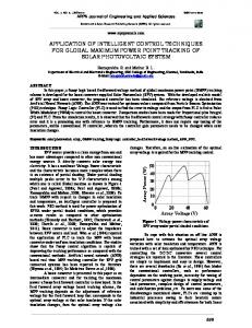
3. FACT Architecture Our overall approach, illustrated in Fig. 1, is centered on model-based approaches to design hybrid observers, fault detection and isolation algorithms, and controller selection and reconfiguration methodologies. Hybrid models [2], derived from hybrid bond graphs [3], which systematically incorporate continuous system dynamics and discrete events, establish the core of the modeling framework. Hybrid observers estimate the continuous dynamic states of the system and detect mode changes in the system operation. Sophisticated signal analysis and filtering methods linked to the hybrid observers will be used for detecting deviations from nominal behavior and triggering the fault isolation schemes.

Figure 1: Fault Adaptive Control Architecture Our diagnostic schemes integrate the use of failurepropagation graph based techniques for discrete-event diagnosis [4] and combine qualitative reasoning and quantitative parameter estimation methods for computationally efficient fault isolation [5] of degraded components (sensors, actuators, and plant components). The dynamic system state accumulated from the observer (discrete system mode plus continuous state vector) and fault isolation units (status of faulty and degraded sensors, actuators, and plant components) define the active system state model. The tracking, fault detection, and fault isolation mechanisms, illustrated on the left of Fig. 1, together constitute a bottom-up computational approach for estimating the dynamic system state (nominal or faulty) by monitoring plant and controller variables. The reconfiguration controller uses this information to select from the controller library the controller that is most effective in maintaining desired system operation and per-

formance. This requires the definition of metrics and decision criteria that govern the controller selection process. The selection and reconfiguration mechanisms operate in a top-down manner, using the dynamic state information to effect changes in supervisory control mechanisms, selection (not synthesis) of feedback control mechanisms, and re-tuning of low level regulators, such as PID or modelbased controllers. The overall computational architecture combines the bottom-up and top-down computational schemes in a seamless manner, via the shared active model. To implement and support the FACT architecture we have used our model-integrated computing tools [1]. We are in the process of building a toolset consisting of a graphical modeling environment, and a set of run-time components. The modeling environment will allow us to create models of the plant (using the modeling approaches described below), and to synthesize implementation code that, when integrated with the generic FACT run-time components will instantiate the architecture for a specific application domain.

3.1 Approaches to fault detection and isolation A primary component of our system is the model-based fault detection and isolation subsystem that can deal with sensor, actuator, and parametric faults in the system. Traditional FDI methods are mainly directed toward sensor and actuator faults. Numerical techniques for state and parameter estimation often face convergence and accuracy problems when dealing with models that have strong nonlinearities [12,13]. Furthermore, these schemes are applicable in continuous real-valued spaces, and they do not easily extend to situations where mode transitions cause discontinuous changes in the system models and system variables. Discrete-event based diagnosis techniques have been proposed, but they require the pre-compiling of the fault models and fault trajectories into finite state automata for tracking nominal and faulty system behavior [14,15]. These approaches have been successfully applied to wellstudied and well-understood systems. For example, finite state machine (FSM) models for tracking the system can be constructed from FMEA documents and historical data collected from the system. In other situations, they may be derived by simulating the detailed system model under a variety of scenarios, and then compiling the information generated into a FSM representation. In both cases, compiling FSM models can be very expensive, and a new FSM has to be generated whenever a new fault is added to the system, or the system configuration is modified. Besides, situations may arise when the discrete-event models are not sufficiently fine-grained to capture small degradations in components that do not produce immediate significant changes in system behavior, but the long-term effects may be very undesirable.

We propose two approaches to the FDI problem that generalize traditional approaches: (i) the use of a robust qualitative fault isolation scheme based on tracking fault transients combined with a parameter estimation scheme for refining fault hypotheses, and (ii) fault diagnostics based on discrete event models represented as fault propagation graphs. We discuss each of these methodologies in greater detail next.

3.2 The continuous approach 3.2.1 Modeling the Plant In our work, we assume the plant is made up of components, such as tanks and pipes that exhibit continuous behaviors. Other components like valves and switches that can be turned off and on at rates much faster than the normal dynamics of the plant. There are also components, such as pumps and motors that exhibit continuous behaviors, interspersed with more discrete on/off transitions. Plants that exhibit these mixed continuous/discrete behaviors are modeled as hybrid systems. Our approach to modeling the plant involves building hybrid automata that combines finite state machines with continuous representations [10]. The FSM, whose states correspond to the modes of operation of the system, captures the possible mode transitions in the system. A continuous system model that governs behavior evolution in that state augments each FSM state. The number of modes of a system may be large enough to make it infeasible to exhaustively generate the complete hybrid automata. We avoid this computational problem by enumerating states of the hybrid automata (which correspond to the modes of system operation) dynamically as system behavior evolves. We use the model of the controller and the direction of change of the system variables to predict possible mode transitions from the current mode of operation. Similarly, the controller model provides indications of all possible controlled transitions from the current mode. The combination of the two sets of constraints results in a small number of possible next modes, making it feasible to pre-compute the continuous models for the corresponding destination states. Conditions for transition to the destination state, and the reset conditions (i.e., the state vector value) in the new state are also pre-computed [11]. We use bond graphs as the modeling paradigm in the continuous domain [12]. Bond graphs represent energybased models of the system in terms of the effort and flow variables of the system. Bonds specify interconnections between elements that exchange energy, which is given by the rate of flow of energy, power = effort x flow. Bond graphs represent a generic modeling language that can be applied to a multitude of physical systems, such as electrical, fluid, mechanical, and thermal systems. There exist standard techniques to build bond graph models of systems based on physical principles. State equations can be sys-

tematically derived from the bond graph representation of the system. In addition, we can also systematically derive temporal causal graphs from bond graphs. This is very important since state equations can be used to simulate system behavior and state equations and temporal causal graphs constitute our diagnosis models. We use an enhanced form of bond graphs that allow controlled junctions that facilitate the modeling of discrete mode transitions in system behavior [3]. In general, the number of modes and possible transitions in a system model can be quite large. Instead of pre-enumerating the bond graph for each mode to build complete hybrid automata, the complete system model is developed as a hybrid bond graph, where individual junctions model local mode transitions [18,19]. The switching 0- and 1- junctions represent idealized discrete switching element that can turn the corresponding energy connection on and off. The physical on/off state for each of these controlled junctions is determined by external control signals and continuous variables crossing pre-specified thresholds. These can be specified as finite state sequential automata. 3.2.2 Fault Detection and Isolation

u Hybrid models

System

y

r

Observer and mode detector

mi Fault isolation

fh

Qualitative analysis Quantitative parameter estimation

Fault detection (Binary decision) Diagnosis models

u = inputs, y = measured output from system,  = predicted output from model, r = residual y – Pi = current mode, fh = fault hypotheses Figure 2: Fault Detection and Isolation Schematic Our diagnosis methodology illustrated in Fig. 2 consists of three mains steps, (i) using a hybrid observer to track system behavior, (ii) detecting fault occurrences, and (iii) isolating faults in the system. The hybrid observer uses the models of the system to track system behavior. We use hybrid bond graphs [3] as the primary modeling language for building hybrid system models. The observer uses the state equations models —derived automatically from the

bind graph models— for tracking continuous behavior in a mode, and the hybrid automaton for detecting and making mode transitions as system behavior evolves. Detection of mode changes requires access to controller signals for controlled jumps, and predictions of state variable values for autonomous jumps. If a mode change occurs in the system, the observer switches the tracking model (different set of state space equations), initializes the state variables in the new mode, and continues tracking system behavior with the new model [18,19]. The fault detector compares the observations from the system and the predictions from the observer to look for significant deviations in the observed signals. We use a simple decision scheme that signals a fault, if the discrepancy between an observation and prediction exceeds a pre-specified threshold for a few time steps, or if an abrupt change is detected in a signal value that cannot be explained by a mode change [14]. Once the fault has been detected, qualitative and quantitative techniques are used to isolate the fault in the system. We use temporal causal graphs [11] derived from hybrid bond graphs for the qualitative analysis, and state equations derived from bond graphs for the quantitative analysis [11,21]. In the qualitative analysis, we first identify an initial candidate set to explain the discrepancy in the observations and predictions. This is achieved by back propagating the qualitative value of the discrepancy (-, 0 or +) through the temporal causal graph of the system. The back propagation may have to be continued in previous modes to identify all possible candidates [15]. We can qualitatively predict future behavior of the system under each of the hypothesized fault conditions by forward propagating through the causal graph. These predictions include magnitude and higher order derivatives of the variables of the system. The predictions can be compared against the qualitative value of the observations to refine the candidate set. We use a technique called progressive monitoring [15] to achieve this. For the quantitative analysis, we estimate the deviated parameter values for each of the remaining fault candidates. To do this, we rewrite the state space equations in terms of the parameter associated with the fault candidate and use system identification techniques to estimate the parameter value [5]. These estimated parameter values could be used to quantitatively predict future behavior of the system, which can be compared to the observations from the system to eliminate some candidates.

3.3 The discrete approach 3.3.1 Failure Propagation Model For discrete diagnosis, the system dynamics is modeled as a tuple (T, L) where T is a set of transition events and L is an event ordering relation. L ⊆ T × T, defined as L = { | there is a transition in which τ2 immediately follows τ1 and τ1 ≠ τ2}.

A transition event represents either a discrete-state transition, or the crossing of a partition boundary in a continuous state space. The tuple (T,L) models the system dynamics, while additional information about the system, such as what outputs are observed when a transition event occurs, or which components are involved in a particular transition event, can be introduced by relations mapping T onto these sets. A subset Tf ⊆ T may be designated as set of fault events. The failure propagation relation, P ⊆ L is defined recursively as P = {∈ L | (τ1∈ Tf ) ∨ (∃τ [ ∈ P] ) }. A Failure Propagation Graph (FPG) is a digraph with vertices V ⊆ T, representing the relation P. A Timed Failure Propagation Graph is an FPG whose edges are labeled with the timing intervals: (tmin, tmax) with the values denoting the minimum and maximum elapsed time between the two transition events at the adjoining vertices. We are now ready to introduce the Failure Propagation Model. A Failure Propagation Model is a 8-tuple (V, E, F, D, A, T, W, Q), where (V, E) is a directed graph (whose vertices are interpreted as transition events), called the failure propagation graph, F is a finite set (whose elements are interpreted as failure modes), D is a finite set (whose elements are interpreted as discrepancies), A is a subset of D (whose elements are interpreted as alarms), T is a relation T ⊆ V× ℘(F) representing a map from sets of failure modes to transition events, W is a relation W ⊆ V× ℘(D) representing a map from sets of discrepancies to transition events and Q ⊆ W, is a relation Q ⊆ V × ℘(A) representing a map from sets of alarms to transition events. We need to consider a mapping between sets of inputs, outputs and faults in order to model observations and faults that are not necessarily independent [16]. The semantic precision of this definition of Failure Propagation Graphs makes it possible to generate the model directly from system models, such as Finite State Automata [16] or timed discrete-event models of quantized systems [17]. However, it is possible to perform diagnosis directly on the Failure Propagation Model, which makes it acceptable as a modeling language, in situations when the complete system model, which includes failure conditions is not known, but typical failure trajectories can be identified. For a system modeled as a Finite State Automata (X, Σ, δ, x0, Y, λ), where X and Σ are the finite state and event sets, x0 is the initial state, and δ: X × Σ × X is the transition function. A transition event can be defined as τ = where σ is a triggering event, x is a state, and δ(σ, x) is the next state. The event-ordering relation is then L = { | ∃σ1,σ2[(τ1 = ) ∧(τ2 = )∧ (x2=δ(σ1, x1))} Given a set of faults modeled as inputs Σf ⊆ Σ, the set of failure transition events is Tf = { ∈ T | σf ∈ Σf }

In this case a mapping can be identified between a failure mode σf ∈ Σf and any transition event τ f =. Alarms, which are events produced by sensors, are associated with outputs, for a Moore machine, in which an output is associated with a state. An output, ya is mapped to any transition τa= for which λ(δ(σ, x))= ya. In a similar fashion, discrepancies, which are unobserved fault conditions, can be mapped to states or transitions. For an FSA of a component constructed from the multiple FSA-s of its components it is also possible to label discrepancies as pertaining to specific components, based on the composition of the system. Any transition in the composed system corresponds to a transition in one or more of components’ FSA-s. 3.3.2 Diagnosis Algorithm Based on the Failure Propagation Model described above, diagnosis can be performed using the predictor-corrector principle [4]. A hypothesis set is maintained, and when a new alarm set is generated, it is compared to the predicted alarms, based on the Failure Propagation Model, and the hypothesis set is updated accordingly. The refined set will contain hypotheses that are compatible both with the observed data and the prediction. 3.3.2.1 Characterizing a Hypothesis The fault propagation graph describes how faults propagate to unalarmed discrepancies and alarms. At any time it is possible to hypothesize any combination of finite paths on the graph as an explanation to the current observation and passed observations. In diagnosis we are not interested in which path led to the current observation, so long as the faults hypothesized are the same. A set of faults is sufficient to identify an explanation for the observed alarms. In conclusion, a hypothesis will be a relation H ⊆ F × V, relating node sets that are consistent with previous and current observations with failure modes that explain them. 3.3.2.2 Hypothesis Set Refinement Each hypothesis consists of a set of faults and a set of current nodes. When a new event is reported, as a new set of alarms, A2 a new set of hypotheses, H2 is generated which would explain each hypothesis in terms of a previous hypothesis, H1 or solely in terms of new faults, or as a combination of both. Hypotheses, which cannot be used to explain the new event, can be ruled out. 3.3.2.3 Calculating a new hypothesis set We will employ the interpretation such that when a failure mode and an alarm are associated with the same transition event, the failure mode provides an explanation for the alarm. This implies that an effect of a failure mode may be

immediate, with no time delay. In other words, there may be failure modes, which are directly observable. A new hypothesis Hk must satisfy the following conditions: (1) All transition events represented in Hk must correspond exactly to the observed alarm set. The transition events in Hk must be in (Q; Ak) where the semicolon represents a relational product [20]. (2) All Failure Modes sets represented in Hk must be some disjunction of a. Failure mode sets from Hk-1, associated by relation Hk-1 to transition events, which are predecessors (by relation P) of the transition events in Hk b. Any set of failure modes, which map (by relation T) to transition events in Hk First we shall address (2). When an event is reported it must be explained by the combination of the previous observation and some (possibly empty) set of new faults. The relation T represents all failure modes associated with their corresponding failure mode instances. The relation P;Hk-1 represents previously hypothesized failure mode sets associated with transition events, which are successors of previously hypothesized transition events. We define the disjunctive superposition of two relations, R1 and R2 as R1 ◊ R2 by

R1 ◊ R2 = { s | (s∈ R1) ∨ (s ∈ R2) ∨ ∃s1, s2[(s1 ∈ R1) ∨ (s2 ∈R2) ∨ (s =s2 ∪ s3 )}

The disjunctive superposition operation represents the possibility of combining any previously hypothesized failure mode sets with any new (or repeated) failure mode sets. The disjunctive superposition T ◊ (P;Hk-1) gives all the combinations of current transition events that can be hypothesized, and relates each such set to a set of failuremodes that explains it. This result must be constrained by (1) resulting in the following formula, using • to denote a join: Hk = (T ◊ (P;Hk-1)) • (Q; A2) The join constrains the set of 2-tuples given by T ◊ (P;Hk-1) to include only those 2-tuples in which the second element (i.e. the transition-event set) is in Q; A2. This formula calculates all possible successor transition events, from the previous hypothesis and associates them with failure mode sets, previously hypothesized. It then finds all combinations of such failure mode sets with new failure mode sets and constrains the resulting set of combinations only to failure mode sets associated with transition events that would produce the observed set of alarms. Thus it predicts the next transition event from the previous hypothesis and corrects the prediction by constraining the hypothesis set to produce the observed alarms.

3.4 Controller selection Our approach is to develop a library of controllers, which will be indexed by sets of characteristics. The goal is to use the information about current system state, i.e., the current mode of operation and system state vector along with failed and degraded states of components and subsystems to select a controller that best suits current and long term performance objectives. This will require the development of efficient encoding schemes for the operational space of system behaviors and constraints that govern system performance. Sophisticated search algorithms will have to be developed for controller selection and reconfiguration. We are addressing the controller reconfiguration task at two levels. At the supervisory (discrete) level, reconfiguration implies modification of high-level control actions. This can take the form of replacing a current action sequence by a new sequence, or altering the sequencing of actions in the current set. This type of reconfiguration requires that the supervisory control logic be explicitly represented as a data structure. Our challenge is to adopt model-based approaches to representing supervisory control programs, and to develop reconfiguration procedures governed by different kinds of fault conditions. At the lower (continuous) level of control, the system relies on regulators, which can range from simple switching controllers to PID mechanisms to model-based controllers. (This is obviously not an exhaustive list.) Reconfiguration at this level can take on three different forms. 1. Set point changes for handling simple fault situations, such as a partially degraded component.

2. Controller tuning for handling cases where the fault changes the plant dynamics (e.g., changes in the capacitive and inertial parameters in the plant), and the retuning of the controller is a viable solution.

3. Structural changes (i.e., rewiring or replacing the regulators) may compensate for complex faults where the current controller architecture is unable to maintain the desired control because of a significant fault (e.g. sensor fault, actuator fault, major structural change in the plant, such as a pump failure or a valve stuck at closed). The switching of controllers in plant feedback loops is discussed in greater detail in the next section. All of the above cases may lead to the introduction of large switching transients into the system. We are investigating two ways to manage the reconfiguration. 1. The Blender approach. In this technique, a “new” controller gradually replaces the “old” controller. Upon the start of the reconfiguration, the old and new controllers are connected to a tapered switch, which initially connects the output of the "old" controller to the plant. As time proceeds, the switch is gradually moved from the old to the new controller. At the end of the

process, the controller completely replaces the old one. Interesting research issues that we have to deal with here, include design of the blending function for control signals at intermediate stages of the tapered switching process and the speed (and thus the dynamics) at which the switching is accomplished to avoid unnecessary transients in the plant dynamics during the reconfiguration process. 2. The State Initialization approach. If rapid reconfiguration is required, the tapered switch approach may not be fast enough. In this case, the new controller should replace the old one, possibly within the sampling interval set for the system. To avoid large bumps, the internal state of the new controller should be initialized in such a way that it generates a control signal after reconfiguration that is minimally different from the last signal generated by the old controller. We will investigate how these initial states of the new controller can be calculated based on the state of the old controller, and the state of the plant. There is an interesting and highly relevant aspect of controller reconfiguration that may need to be addressed in a later stage of the project, i.e., explicit management of reconfiguration transients. Early results [24,25] show that there are a number of techniques available for mitigating reconfiguration transients in control systems. If the proposed approach of controller re-initialization and/or blending does not meet the requirements for the reconfiguration dynamics other, explicit transient suppressions techniques can be applied to mitigate the effects of switching.

3.5 An application domain: aircraft fuel system Modern aircraft are equipped with sophisticated control systems in support of their fuel systems. The fuel system consist of a number of tanks, interconnecting pipes, valves, and pumps, whose tasks are manifold. First, the system should supply fuel to the engines under all flight conditions. Second, the center of gravity of the aircraft has to be maintained. To achieve this, the fuel may have to be pumped from tank to tank during flight. Third, in case of failures (e.g. pump failures, leakage in the tanks, valves getting stuck), the system should utilize the built-in redundancy to compensate for the failure, and to maintain control. We are currently working on creating models of a generic aircraft fuel system, and testing the FACT tools and techniques we have developed with the help of this example.

4. Results, Conclusions and Future Work We have applied our continuous and discrete FDI methodology to diagnosing faults in a three-tank system with a number of valves. A simple supervisory controller model was implemented that took the system through a number of tank filling, emptying, and mixing cycles. We were successful in tracking continuous system behavior through

discrete mode changes, and isolating faults when the occurred, with the discrete and continuous diagnostics algorithms. As a next step, we would like to extend the two diagnostic algorithms to work in a more cohesive fashion, and inform each other as they come up with fault hypotheses. The idea is to come up with schemes where we can track and analyze behaviors of complex systems at multiple levels of detail. Once this step is completed, we will integrate in the controller selection mechanisms to complete our implementation of the FACT architecture that has been presented in this paper.

Acknowledgements The DARPA/ITO SEC program (F30602-96-2-0227), and The Boeing Company have supported the activities described in this paper. We would like to thank Dr Kirby Keller and Mr. Mark Kay for their help.

References [1] Sztipanovits, J., Karsai, G.: “Model-Integrated Computing”, IEEE Computer, pp. 110-112, April, 1997. [2] Branicky, M.S., V. Borkar, S. Mitter, 1994. “A Unified Framework for Hybrid Control: Background, Model, and Theory,” Proceedings of the 33rd IEEE Conference on Decision and Control, Lake Buena Vista, FL, Paper No. LIDS-P-2239. [3] Mosterman P.J. and G. Biswas, 1998. “A theory of discontinuities in physical system models,” Journal of the Franklin Institute:335B, pp. 401-439. [4] Misra A., Sztipanovits J., and Carnes J., 1994. “Robust Diagnostics: Structural Redundancy Approach,” Knowledge Based Artificial Intelligence Systems in Aerospace and Industry, SPIE's Symposium on Intelligent Systems, Orlando. [5] Manders E.J., S. Narasimhan, G. Biswas, and P.J. Mosterman, 2000. A combined qualitative/quantitative approach for efficient fault isolation in complex dynamic systems. 4th Symposium on Fault Detection, Supervision and Safety Processes, pp. 512-517. [6] Patton, R.J., Frank, P.M., and Clark, R.N. (eds.), 2000. Issues of Fault Diagnosis for Dynamic Systems, SpringerVerlag, London, U.K. [7] Chen, J. and Patton, R.J. 1999. Robust Model-Based fault Diagnosis for Dynamic Systems, Kluwer Academic, Boston, MA. [8] Sampath, M. et al., 1996. “Fault Diagnosis using Discrete-Event Models,” IEEE Trans. On Control Systems Technology: 4(2), pp. 105-124. [9] Lunze, J. 1999. “A Timed Discrete Event Abstraction of Continuous Dynamic Systems,” Intl. Journal of Control: 72, pp. 1147-1164. [10] Alur, R. et al., 1993. Hybrid Automata: an algorithmic approach to the specification and verification of hybrid

systems, in, R.L. Grossman, et al., eds., Lecture Notes in Computer Science, Springer, Berlin, 736, pp. 209-229. [11] Narasimhan, S. and Biswas, G. 2000. Using Supervisory Controller Models for more Efficient Diagnosis of Hybrid Systems. Submitted to Hybrid Systems: Control and Computation, Intl. Workshop, Rome, Italy. [12] Rosenberg, R.C. and Karnopp, D.C. 1983. Introduction to Physical System Dynamics, McGraw Hill, NY. [13] Narasimhan, S., Biswas, G., Karsai, G., Pasternak, T., and Zhao, F., 2000. “Building Observers to Handle Fault Isolation and Control Problems in Hybrid Systems,” Proc. 2000 IEEE Intl. Conference on Systems, Man, and Cybernetics, Nashville, TN, pp. 2393-2398. [14] Manders E.J., Mosterman, P.J., and Biswas, G., 1999. Signal to symbol transformation techniques for robust diagnosis in TRANSCEND, Tenth International Workshop on Principles of Diagnosis, Loch Awe, Scotland, pp. 155165. [15] Mosterman P.J. and Biswas G., 1999. Diagnosis of Continuous Valued Systems in Transient Operating Regions, IEEE Trans. on Systems, Man and Cybernetics:29, pp. 554-565. [16] Pasternak, T. Extended Relational Models for Diagnosis, Masters Thesis, Vanderbilt University, August 2000. [17] Lunze, J., Diagnosis of Quantized Systems by Means of Timed Discrete-Event Representation, in Proc. Of Thirds International Workshop on Hybrid Systems, Computation and Control, Lecture Notes in Computer Science, volume 1790, pages 258-271, March 2000. [18] Simon, G., Kovácsházy, T., and Péceli, G., 2000. “Transients in Reconfigurable Control Loops,” IEEE Instrumentation and Measurement Technology Conference, IMTC/2000, Baltimore, Maryland, USA. [19] Simon, G., Kovácsházy, T., and Péceli, G., 2000. “Transient Management in Reconfigurable Systems,” International Workshop on Self Adaptive Software, Oxford University, England. [20] Pierce, C. S. "Note B: The Logic of Relatives." In Studies in Logic by Members of the Johns Hopkins University Boston: Little Brown and Co. 1883