Fault-Detection and Fault-Tolerant Design for Microfluidicbased Biochips Yu-Chih Chen
Win San Vince Khwa
Ming Han Victor Yu
Department of EECS University of Michigan
[email protected]
Department of EECS University of Michigan
[email protected]
Department of EECS University of Michigan
[email protected]
different configurations of defective cells in order to simulate real-time behaviors of Microfluidics-based biochips. Two new detection algorithms (binary partition and local-detouring) have been implemented and compared with contemporary alternatives. The second priority is fault-tolerance, in which we plan to implement an algorithm to reconfigure module placement when defects occur. In complex designs, multiple defects are prone to occur concurrently. We will consider different arrangements of defective cells that may arise at runtime. Once defective cells are identified, automatic recovery techniques are essential. A design based on partial reconfiguration to avoid faulty cells has been suggested [4]. This scheme, however, requires the presence of large number of unused cells in the array, which suffers from area overhead. Moreover, it does not address situations with multiple defects, which we include in our design. We show in this paper that by implementing a more effective defect detection algorithm, biochips can be reconfigured to function for a longer period of time.
ABSTRACT Microfluidic-based biochips are often used in safety-critical applications, in which reliability is one of the most essential design metrics. In order to recover from erroneous operations, fault-tolerance is a desirable feature for these devices. Designing fault-tolerant biochips requires two steps: fault-detection and fault-recovery. Despite the strong dependency between these two steps, current researches often consider them as separate problems by neglecting their correlations. Our project focuses on proposing a design that attempts to combine fault-detection and faultrecovery to mitigate the reliability problem in microfluidics technology. Experimental results illustrated that our proposed detection method, comparing with contemporary alternatives, significantly improved the detection coverage and the chance to recover from runtime errors for larger size biochips.
Keywords Microfluidic, fault detection, fault tolerance.
2. Related Prior Works
1. INTRODUCTION
Several fault-detection algorithms have been proposed by researchers. This section will briefly discuss three algorithms relevant to our project – parallel scan, diagonal scan, and binary search.
Microfluidics-based biochips are microsystems that integrate several repetitive laboratory procedures onto a single chip. The architecture of the device is based on a two-dimensional array of electrodes (unit cells) that are used to manipulate discrete droplets, which are typically in nanoliter volumes. These miniscule biochips, usually in the range of square millimetres, have enabled on-chip immunoassays, DNA analysis, environmental toxicity monitoring, and many other fields in molecular biology [1]. Microfluidics technology offers many advantages over traditional laboratory methods, which include reduced volume consumption of fluids, faster processing speed, and lower costs due to the ability for mass production [1].
2.1 Parallel Scan Parallel scan-like test was first introduced by Tao Xu and Krishnendu Chakrabarty in 2007. The key idea is to manipulate multiple droplets in parallel to test the microfluidic array in a scan-like manner [2]. Prior to parallel scan, fault-detection was performed by single droplet scan test. One major drawback of single droplet testing is that its test time may be excessive for large arrays. Tao et al proposed that the scanning test can be done in parallel by using multiple droplets. Figure 1 illustrates both test methods.
Since microfluidics-based biochips are often used in safetycritical applications, reliability is one of the most important design metrics. In order to recover from erroneous operations, these devices need to be designed for fault-tolerance. Moreover, as the complexity of microfluidics-based lab-on-chip increases, defect density is expected to increase. As a result, efficient runtime recovery techniques are necessary. Designing fault-tolerant biochips requires two steps: faultdetection and fault-recovery. Even though there is a strong dependency between these two steps, current researches often consider them as separate problems by neglecting their correlations. Furthermore, most research [2], [3] focused on testing for correctness and searching for sources of defects. Works related to fault-recovery are limited, even though it is crucial in complex designs.
Figure 1. Single droplet scan (left) and Parallel scan (right).
We proposed a design that combines fault-detection and faulttolerance to mitigate the reliability problem in microfluidics technology. Our first priority is fault-detection. We consider
For parallel scan, droplets are manipulated in alternative rows/column because sufficient spacing between droplets must be
1
Both problems can be mitigated by performing the diagonal scan test after the parallel scan test. In this test, multiple droplets are to transverse the array in diagonal manner. Figure 5 shows the paths of droplets in a diagonal scan test.
maintained to avoid unintentional merging of droplets [5]. This implies that a total minimum of four iterations for vertical and horizontal scans are needed. In order for the parallel scanning to proceed, the first step is the transport the droplet from pseudosource to the starting position in alternative rows/columns. For this reason, a peripheral test is implemented to verify the cells on edge (Figure 2). Afterward, two iterations of column test and row test are performed. Based on the test outcomes, the location of the defect can be determined.
Figure 5. Illustration of diagonal scan test.
2.3 Binary Search The binary search algorithm is implemented by Su et al. to determine the location of defective cells [6]. The method proceed by first manipulate two droplets to traverse in opposite direction toward the defect by half the array size (N/2). If the droplet is unable to complete the round trip, detect is found in this path. The depth of the broken path is reduced by 2 , where n is the value for current iteration. Its complementary path is increased by the same amount. The bidirectional round trip test is repeated for times. The outcome of the tests can be interpreted to defect location.
Figure 2. Illustration of peripheral test.
2.2 Diagonal Scan The parallel scan method mentioned above has some disadvantages. As the cell fail rate or the array size increases, it can some time report back the incorrect defect location. Furthermore, there exist some unreachable sites on the biochip [2]. Incorrect defect location can happen when there are multiple defects in the array. Figure 3 below illustrated one possible instance such that incorrect defect locations can be reported.
Figure 6 below is an example of how to locate a defective cell on a 8x8 array. First, two droplets are manipulated to traverse toward the defect with depth value of four. It is found that the bottom chain is broken. In the second iteration, the depth of the top and bottom droplet is modified to six and two, respectively. Similarly, the third iteration is done with depth five and three. By converting the binary result for each droplet to integer, we can determine the detect location is five cells (101 = 5) below and two cells above (010 = 2).
Figure 3. Example of reporting incorrect defect locations. Unreachable sites on the biochip are another major concern. A cell can become unreachable if there are defects in all four directions. Figure 4 below demonstrates this situation. Figure 6. Illustration of binary search.
3. Problem Formulation 3.1 Assumptions As previously described, the biochip is modeled as a twodimensional array of cells. These cells are formulated by using a graph. Each cell is a vertex and the connection between cells is defined as an edge. There are two types of errors: vertex error and edge error. The former represents that a cell cannot transport drop to any neighboring cells. The latter means the path between two cells failed (can be either a short or an open). Modeling a biochip has the potential of becoming extremely complex; several assumptions were made to simplify our system. First, we assumed
Figure 4. Example of unreachable cell.
2
the peripheral tests (Figure 2) of each chip are successful. Second, pseudo sources and pseudo sinks are defect-free. These two assumptions are required to keep the detection complexity down. Furthermore, they are also enforced in most reference papers we have surveyed so far. Lastly, we will only consider vertex errors and omit edge errors. The justification is that the probability of pure edge error is quite low comparing to that of vertex error. The latest papers also concentrate the discussion on vertex errors.
single defect on a biochip due to the small size of the chip. Since the size of biochips is anticipated to increase, the number of defects is expected to rise too. The third conceptual novelty is integrating fault-detection and fault-tolerance. Current related works [1-6] either focus on one problem or the other. However, due to their interdependencies, they must be considered together in order to design a completely reliable biochip. The next subsection addresses this topic.
3.2 Defect Modeling
The three experimental innovations, namely defect detection, module placement, and module reconfiguration, are detailed in the next three sections. This paper proposes two defect detection algorithms that provide more detection coverage than existing methods do. Moreover, a fast module placement technique is described. Finally, unlike other recovery mechanisms that account for just one defect, a fault-tolerant scheme has been designed to tolerate multiple defects.
3.2.1 Fabrication Defects Another challenge is formulating a realistic defect model. It is a heuristic to assume defects are uniformly distributed across the biochip. In reality, however, defects actually occur close to one another. Any model that ignores the clustered defect pattern may risk grossly underestimating the true yield [7]. To implement the clustering effect into our model, we will distribute the defects in two iterations. In the first round, defects are uniformly distributed across the chip. Afterward, a second iteration of Gaussian defect distribution is performed on each defect location from the first iteration. To keep the amount of defects similar to that generated by pure uniform distribution, the rate of cell failure (Pc) during the first iteration is scaled down by a factor.
4.2 System Overview Figure 8 illustrates the systematic overview of the proposed design of fault-detecting and fault-tolerant biochips. First, a biochip is manufactured with fabrication defects present on chip. The biochip is checked for defects using any fault-defection algorithm. Module placement is then performed using a clientspecified microfluidic module library. Afterward, runtime defects occur continuously. Modules containing runtime defects are reconfigured to new locations to avoid using the defective cells. During field operation, the biochip must be periodically checked for runtime defects. Hence, module reconfiguration repeats until it fails, in which case the fabricated biochip must be discarded [4].
3.2.2 Runtime Defects After a thorough study of existing works, data related to runtime defects of biochips could not be found. Hence, a new model must be assigned. Reliability engineers often model failure rates of products over time using the bathtub curve, as seen in Figure 7. When customers begin using products, many failures, known as early failures, manifest themselves immediately but at a decreasing rate. Next, failure rate levels off and remains roughly constant. This region, which accounts for most of the product’s useful life, is characterized by random failures. Finally, materials eventually degrade and wear out at an increasing rate. Since many engineering products, such as microprocessors and integrated circuits, reflect the bathtub curve, we assume that the failure rate of biochip cells can also be characterized by the same curve.
Figure 8. System Overview of Proposed Design.
5. Defect Detection Figure 7. Bathtub Curve for Engineering Products.
5.1 Binary Partition When the size of array grows larger or the error rate becomes higher, most cells are blocked by defects. We cannot locate these defective cells using parallel or diagonal detections. Although most of these cells are correct, they are useless. Figure 9 is an array with a high error rate. We can see that the central region is blocked and therefore generates many undetectable cells.
4. Our Contributions 4.1 Novelties The paper investigates three conceptual novelties and implements three experimental novelties. The first conceptual novelty involves experimenting with large arrays of cells, such as 512 x 512. Conventional approaches [1-6] often limit themselves with small arrays, such as 8x8 and 10x10. Given the improved manufacturability of biochips and their potential to be used in more applications, more cells are required to perform more complex functions and to perform more functions concurrently. The second conceptual originality is addressing multiple defects simultaneously. Existing research [1-6] are constrained with just a
3
Figure 9. Example of a high error rate array. To deal with this problem, we try to partition the whole array into small sub-arrays. Then, we can detect the cells more easily and thus reducing the number of undetectable cells. Hence, we separate the array by defect-free columns or rows.
Figure 11. Operation of local detouring This method is effective because the probability that all three routes (one original straight route and two local detouring routes) are blocked is much lower than Pc. We can define a new Pc` based on statistical analysis seen below.
First, we find defect-free columns by parallel scanning. If there is at least one fault-free column, we separate the array by the column which is closest to the center. If there is no such fault-free column, we can try to partition it by a defect-free row. Since we partition it by a fault-free column, the droplet can move to the periphery of sub-arrays. Then, we can do parallel scanning and binary search on the sub-arrays. If there are still some undetectable cells, we repeat the same process on rows of sub-arrays. The binary partitioning is to be repeatedly executed until one of the following two conditions is matched: (1) the entire sub-array has no undetectable cells or (2) each row/column has at least one defect. Figure 9 is a good example of binary partition, if we partition the array by the central column, all the cells are detectable.
Pr Pr
Pr 1
1
The values of Pc’ are given in Table 1. The new Pc’s are much smaller than original Pcs, which suggest that the local detouring approach is a powerful technique for reducing the undetectable area. Table 1. Comparison of Pc and Pc’.
5.2 Local Detouring Binary partition can reduce the number of undetectable cells. However, when the error rate is too high or the size is too large, each row/column is blocked by at least one defect. In this case, binary partition is useless. Figure 10 demonstrates the case that each row/column has at least one defect.
Pc
0.005
0.01
0.02
0.03
0.04
0.05
Pc’
2.0E‐6
1.6E‐05
1.2E‐04
4.0E‐04
9.1E‐04
0.0017
Pc
0.06
0.07
0.08
0.09
0.1
0.11
Pc’
0.0029
0.0044
0.0064
0.0089
0.012
0.015
5.3 Reducing Runtime of Error Detection Although the local detouring method can reduce the number of undetectable cells, the slow movement of microfluidic droplets makes the runtime of error detection algorithms extremely critical. To deal with this problem, we achieved a more efficient algorithm by selecting an Initial Traversing Depth (ITD). It is known that for an array size of 512x512 with Pc values larger than 0.02, there is almost no error-free row/column. In most cases, a droplet is blocked by an error within a few moves. The original binary search, which tries to traverse all the rows/columns, is impractical and time-consuming. We aim to reduce the complexity by selecting a proper ITD value. Since Pc can be derived after several testing, we can set an ITD that is proportional to 1/Pc. If the ITD is larger than the farthest error, we can continue with the binary search. On the other hand, when the ITD is smaller than the farthest error, we must select a larger traversing depth and try again. In the original binary search, the ITD is 256 (N/2). We found through experiments that we can reduce the runtime by decreasing this value to a constant times 1/Pc. Selecting a proper ITD, we can greatly reduce the runtime. Figure 16 is an illustration of the impact.
Figure 10. Array without any defect-free row/column. Hence, we design the technique of local detouring as depicted in Figure 11. Once a defect is encountered, we will immediately look for a local detouring route around the defective location. We follow the green route first. If it is still blocked, we can pursue the red route. Unless the original straight route and the two detouring routes are blocked, the defect will not block that column/row. The array in Figure 10 can be partitioned by this local detouring method, and all undetected cells can be detected.
4
perform another perturbation. Since our objective is minimizing the run time of the chip, the cost function is time t plus the penalty of exceeding the array size.
6. Module Placement 6.1 Microfluidic Module Library Performing any analysis using the biochip requires a sequence of different operations. Many of the surveyed research paper define this sequence in a digital microfluidic module library. It would be ideal to implement an actual biomedical process in our system; however, current available libraries are designed for smaller size of biochips. For this reason, we decided to create the library for our 512x512 biochip. The Table 2 below is the library implemented. These module sizes and times are chosen similar to the modules used in a polymerase chain reaction for DNA analysis [4].
In this section, we carry out 10000 sets of operation of Table 2 (total 100000 sequenced modules) on a 512X512 chip. Since the computation is too complex, we need to simplify the algorithm. Instead of considering all the modules at the same time, we first consider 10000 OP1 modules then 10000 OP2 modules and repeat this until all operations are done. It may not be an optimized solution, but this new problem is feasible. Hence, we can use this reduced simulated annealing placer to place the modules.
7. Module Reconfiguration
Table 2. Module library
7.1 Key Parameters
Operation
Module Size
Duration(s)
OP1
4X4
6
OP2
2X4
4
Analogous to the definition of Pc, which is the probability of a cell failure due to fabrication, we define Pcr, which is the probability of a cell failure arising at runtime. We also define the utilization of the biochip to be
OP3
2X4
6
∑
OP4
4X8
4
OP5
6X6
6
OP6
2X2
3
OP7
1X2
2
OP8
1X2
3
The equation states that utilization is the sum of module areas divided by the size of the array. Thus, this relation monitors how “crowded” a given biochip is. Intuitively, the higher the utilization is, the more difficult reconfiguration becomes because the number of unused cells reduce.
OP9
2X4
2
7.2 Partial Reconfiguration
OP10
3X3
3
Our fault-tolerant technique is based on partial reconfiguration, as described in [4] and [9]. In [4], an algorithm was implemented for arrays with just a single failing cell. An enhanced algorithm has been developed to reconfigure multiple defective modules. The reconfiguration procedure first locates a defective cell that arises at runtime. If the cell has been occupied by a module, we traverse the entire array to locate an unused defect-free region that can accommodate that module. If the search is successful, relocation occurs; if not, reconfiguration fails. As long as reconfiguration has not failed, this process continues in order to locate the next defective cell.
6.2 Simulated Annealing Placement Since Simulated Annealing is an efficient algorithm in for placement, we implement a placer of SA. According to [8], we see that T-tree is a good representation of 3D placement. T-tree is a tree structure that each node can have at most three children. Each node represents an experiment module. The root will be placed at the lower left corner of the array. The middle child will be placed on the upper of it and the left child will be placed on the right of it. If a place is occupied by an error, we just move the modules upward or rightward. The parent, middle child and right child will start at the same time, and the left child will start after the parent module has finished. Figure 12 below is an example of a T-tree.
Figure 13. Example of Partial Reconfiguration. Figure 13 shows an example in which defective modules are relocated to unused defect-free cells. Note that healthy modules are not affected by reconfiguration. Figure 12. Example of a T-tree.
8. Experimental Results
The T-tree can do three perturbations: rotate a module, exchange two modules, and exchange two sub-trees. After performing a perturbation, we examine whether the sequence of operations is violated. If the sequence is violated, this new tree is illegal and we
8.1 Experiment Setup Experiments are carried out on Intel® Xeon® 3.00 GHz processor with 4 GB of memory work stations located in Duderstadt Center.
5
As Pc increases, the runtime of parallel and diagonal algorithms will decrease due to the errors being close to each other. On the contrary, the complexity of the local detouring algorithm will increase. This is due to the fact that more partitions are needed when Pc is higher, which lead to a complexity increase. However, this increasing trend is not monotonic; if the Pc is too high, the array can no longer be partitioned. In this situation, the number of steps will drop dramatically. Figure 16 clearly illustrates these phenomena.
The experiments can be categorized into three sections – detection coverage, module placement, and module reconfiguration. Each test is based on a 512x512 biochip array. Detection coverage investigates the impact of various algorithms on chip coverage under both Gaussian and normal defect distribution. In module placement, we compare the processing time required for a specific operation on biochips that have been through different detection algorithms. Lastly, in module reconfiguration, we inject random runtime defects onto the chip and analyze their chances of recovering.
To show the effects of selecting proper traverse depth, we have conducted an experiment for counting the number of steps required in the detection process for various algorithms. As one can see in Figure 16, compared with green line (original local detouring), the yellow line (reduced local detouring) needs much less operations. Since we can carry out detection in many subarrays, the running time is even lower than diagonal approaches.
8.2 Detection Coverage The number of undetected cells over total number cells is the probability of cell being undetectable Pu. In Figure 14, we can see that the binary partition method works better than previous parallel and diagonal methods. However, when the error rate grows higher, binary partition is not so useful. If we turn to the local detouring method, we can improve the performance further.
Figure 16: Runtime comparison of four different error detection methods
8.3 Module Placement
Figure 14: Pu comparison of four different error detection methods under random defect distribution
After defect detection, we use simulated annealing placer to place operation modules on the chip. If a cell is undetected, we cannot use it to do any operation. On the contrary, if we can detect almost all undetected cells, we have more computing resources. Hence, if the undetected probability is lower, we can achieve shorter run time. We can see that run time is a good yardstick to compare the performance among different detection methods. Also, we provide the case of ideal detection which can detect all cells.
If the defect distribution is clustered by Gaussian function, the result is shown in Figure 15. Since the defects tend to cluster together, we can get more defect-free area. Hence, the diagonal and partition approaches get slightly better result. However, it is hard to detour clustered defects. So, the performance of local detouring get worse.
The running time is defined as the time that can finish 10000 set of modules in Table 2. From Figure 14 and Figure 17, it is clear that the higher the undetected area, the longer the running time. If Pc is lower than 0.08, the Local Detouring algorithm can detect almost all cells. Hence, the run time is close to the ideal detection case. Since the parallel and diagonal have much higher undetected area, their running time is much longer.
Figure 15: Pu Comparison of four different error detection methods under Gaussian cluster defect distribution.
6
Percentages of functional chips over time for three different detection algorithms are displayed in Figure 19. Local detouring technique outperforms both diagonal and parallel algorithms. Specifically, using local detouring scheme for detection guarantees that all biochips can survive well into the random failure phase. On the other hand, when utilizing parallel and diagonal algorithms, only 10 percent and 0 percent of biochips can survive, respectively, before entering the random failure phase (time 3).
Figure 17: The run time vs. cell error probability in different detection methods.
8.4 Module Reconfiguration Figure 18 shows the reconfigurability for different biochip utilization rates at different values of Pcr. The experiments were performed using a Pc value of 0.1 in order to account for the worst case scenario during fabrication. For all values of Pcr, reconfigurability either stays the same or decreases as utilization increases, which agrees with our earlier intuition. Moreover, as Pcr increases, reconfigurability either stays the same or decreases (i.e. the curves shift to the left). This observation makes sense because the insertion of more runtime defects hinders the reconfiguration process.
Figure 19. Percentage of Functional Chips Over Time.
9. Conclusion In this paper, we have presented conceptual ideas and developed efficient algorithms to accommodate the next generation of microfluidic-based biochips. In particular, our design focuses on large biochips, addresses multiple defects on chip, and combines fault-detection and fault-tolerance methodologies to form a reliable design for biochips. We have developed effectual faultdetection algorithms that provide better detection coverage, an economic module placing technique that runs faster, and a more powerful module reconfiguration scheme that accounts for multiple defects. In the future, we would like to acquire a more realistic module library, especially for large biochip arrays. Also, we would like to obtain actual failure data for fabrication and runtime. Moreover, we would like to explore the possibility of performing complete module replacement and/or partial module replacement in the event that partial reconfiguration fails.
10. Lessons Learned In this project, we learned a great deal about the basics of microfluidics technology. We learned about the theory behind their operations and some of their applications. The fact that Microfluidic-based biochips combine knowledge from biomedical engineering and Mirco-Electro-Mechanical Systems (MEMS) is very interesting. In addition, we studied current design challenges in microfluidic-based biochips. We realized that current research is limited to small biochips with at most one defect per chip. With the fast growth of micofluidics technology, such constraints are impractical and ironic. Hence, we pioneered new research areas that center on large biochip arrays with multiple defects per chip. We also proposed the idea of performing periodic defect-detection and defect-recovery procedures once the biochip is in field. Furthermore, we learned different tricks to designing efficient defect-detection algorithms.
Figure 18. Reconfigurability vs. Biochip Utilization. The relationship between the effectiveness of the detection algorithm and the expected survival time of the biochip was also investigated. Following the bathtub curve in Figure 7, different values of Pcr were assigned to different time points. The values are listed in Table 3. Table 3. Probability of Runtime Defect at Different Times
Time 1 2 3-11 12 13
Pcr 0.1 0.05 0.025 0.05 0.1
7
Proceedings of Design, Automation and Test in Europe (DATE) Conference, pp.1202–1207, 2005.
We gained some C++ programming skills. Particularly, we became experienced with memory management in object-oriented programming. We encountered and alleviated memory-related issues due to the large size of biochips we were designing. Also, we became more comfortable working in teams. We organized effective team meetings and set appropriate deadlines. As a result, our project was a huge success.
[5]
F. Su and K. Chakrabarty, “Unified high-level synthesis and module placement for defect-tolerant microfluidic biochips”, in Proc. IEEE/ACM Des. Automat. Conf., 2005, pp. 825-830.
[6]
F. Su, W. Mukherjee, and K. Chakrabarty, “Defectoriented testing and diagonosis of digital microfluidicsbased biochips”, in Proceedings of the IEEE International Test Conference, pp. 21.2.
[7]
Bae, Suk Joo, Hwang, Jung Yoon and Kuo, Way. “Yield Prediction via Spatial Modeling of Clustered Defect Counts Across a Wafer Map”, IIE Transactions, 39:12, 1073 – 1083.
[8]
PING-HUNG YUH, CHIA-LIN YANG, and YAO-WEN CHANG, “Placement of Defect-Tolerant Digital Microfluidic Biochips Using the T-tree Formulation”, ACM Journal on Emerging Technologies in Computing Systems, Vol. 3, No. 3,Article 13, Publ. date: November 2007
[9]
T. Xu, K. Synthesis of pp.647-652, Design held Embedded
11. ACKNOWLEDGEMENTS We would like to thank Professor Valeria Bertacco for her guidance throughput the development of this project.
12. REFERENCES [1]
K. Chakrabarty and J. Zeng, "Design automation for microfluidics-based biochips", ACM Journal on Emerging Technologies in Computing Systems, vol. 1, pp. 186-223, December 2005.
[2]
T. Xu and K. Chakrabarty, "Parallel scan-like test and multiple-defect diagnosis for digital microfluidic biochips", IEEE Transactions on Biomedical Circuits and Systems, vol. 1, pp. 148-158, June 2007.
[3]
Y. Zhao, T. Xu and K. Chakrabarty, "Built-in self-test and fault diagnosis for lab-on-chip using digital microfluidic logic gates", Proc. IEEE International Test Conference, 2008.
[4]
F. Su and K. Chakrabarty, “Design of fault-tolerant and dynamically-reconfigurable microfluidic biochips”, In
8
Chakrabarty, and F. Su, "Defect-Aware Droplet-Based Microfluidic Biochips," vlsid, 20th International Conference on VLSI jointly with 6th International Conference on Systems (VLSID'07), 2007