Fault Diagnosis for Rotating Machinery Using Vibration ... - MDPI

sensors Article

Fault Diagnosis for Rotating Machinery Using Vibration Measurement Deep Statistical Feature Learning Chuan Li 1, *, René-Vinicio Sánchez 2 , Grover Zurita 2 , Mariela Cerrada 2 and Diego Cabrera 2 1 2

*

School of Mechanical Engineering, Dongguan University of Technology, Dongguan 523808, China Department of Mechanical Engineering, Universidad Politécnica Salesiana, Cuenca 010105, Ecuador; [email protected] (R.-V.S.); [email protected] (G.Z.); [email protected] (M.C.); [email protected] (D.C.) Correspondence: [email protected]; Tel.: +86-138-0838-1797

Academic Editor: Vittorio M. N. Passaro Received: 13 May 2016; Accepted: 13 June 2016; Published: 17 June 2016

Abstract: Fault diagnosis is important for the maintenance of rotating machinery. The detection of faults and fault patterns is a challenging part of machinery fault diagnosis. To tackle this problem, a model for deep statistical feature learning from vibration measurements of rotating machinery is presented in this paper. Vibration sensor signals collected from rotating mechanical systems are represented in the time, frequency, and time-frequency domains, each of which is then used to produce a statistical feature set. For learning statistical features, real-value Gaussian-Bernoulli restricted Boltzmann machines (GRBMs) are stacked to develop a Gaussian-Bernoulli deep Boltzmann machine (GDBM). The suggested approach is applied as a deep statistical feature learning tool for both gearbox and bearing systems. The fault classification performances in experiments using this approach are 95.17% for the gearbox, and 91.75% for the bearing system. The proposed approach is compared to such standard methods as a support vector machine, GRBM and a combination model. In experiments, the best fault classification rate was detected using the proposed model. The results show that deep learning with statistical feature extraction has an essential improvement potential for diagnosing rotating machinery faults. Keywords: fault diagnosis; deep learning; statistical feature; vibration sensor; rotating machinery

1. Introduction As one of the fundamental types of mechanical system, rotating machinery is widely applied in various fields. As a result of relative motion between mating surfaces, components of rotating machinery are prone to suffer from damage [1]. Effective fault diagnosis is thus important for maintaining the health of rotating machinery. One of the most challenging fault diagnosis tasks is the detection of faults and fault patterns, if any. Different methods have been developed for fault diagnosis in rotating components such as gearboxes and bearings [2–4]. Gao et al. [5,6] systematically reviewed the fault diagnosis with model-based, signal-based, knowledge-based, and hybrid/active approaches. The most successful methods have three main steps: determining the fault symptoms, extracting the sensitive features, and classifying the condition patterns. Various fault symptoms, including vibration measurements [7], thermal features [8], acoustic signals [9], oil debris [10], and other process parameters have been used as indices of the health of rotating systems. Vibration sensor signals have been proven effective for monitoring the health of rotating machinery. Even in the vibration sensor category, different features sensitive to fault detection have been extracted in recent years. Most of these feature extractions are performed in the time domain, Sensors 2016, 16, 895; doi:10.3390/s16060895

www.mdpi.com/journal/sensors

Sensors 2016, 16, 895

2 of 19

frequency domain, and time-frequency domain. To extract a fault feature in the time domain, Raad et al. [11] proposed using cyclostationarity as an indicator to diagnose gears. A diagnostic feature was introduced by Bartelmus and Zimroz [12] to monitor planetary gearboxes in time-varying operating conditions. The fault features are sometimes very sensitive in the frequency domain. Spectral kurtosis is one of the most popular fault features in the frequency domain [13]. Based on frequency domain kurtosis, an optimal mathematical morphology demodulation method was proposed for the diagnosis of bearing defects [14]. Compared to feature extraction in the time and frequency domains, time-frequency domain features have attracted much attention in both academia and industry. Continuous wavelet transform (CWT) [15], discrete wavelet transform (DWT) [16], wavelet packet transform (WPT) [17], second generation wavelet transform [18], comblet transform [19], and other time-frequency tools [20,21] have been successfully used to generate fault-sensitive features. In addition to feature extraction in a single domain, researchers have proposed detecting machinery faults in different domains. Lei et al. [22] proposed two diagnostic parameters from an examination of the vibration characteristics of planetary gearboxes in both the time and the frequency domains. Based on the extracted fault features, different classifiers have been used to distinguish the healthy condition from different fault patterns. A multi-stage feature selected by genetic algorithms was proposed by Cerrada et al. [23] for the fault diagnosis of gearboxes. An intelligent diagnosis model jointly using a wavelet support vector machine (SVM) and immune genetic algorithm (IGA) was introduced for gearbox fault diagnosis [24]. Discriminative subspace learning has been used to diagnose faults in bearings [25]. Tayarani-Bathaie et al. [26] introduced a dynamic neural network to diagnose gas turbine faults. An artificial neural network and empirical mode decomposition have been applied to automatic bearing fault diagnosis using vibration signals [27]. It is clear that the SVM family has achieved good results in comparison with peer classifiers. Recently, deep learning has gained much attention in the classification community. Tamilselvan and Wang [28] introduced deep belief learning based health-state classification for failure diagnosis in datasets including iris, wine, Wisconsin breast cancer diagnosis, Escherichia coli and others. Tran et al. [29] used deep belief networks for the diagnosis of reciprocating compressor valves. In this paper, we present a deep statistical feature learning approach for fault diagnosis in rotating machinery. The purpose of this paper is to use deep statistical feature learning as an integrated feature optimization and classification tool to improve fault diagnosis capability. For deep learning of statistical features with unknown value boundaries, a Gaussian-Bernoulli deep Boltzmann machine (GDBM) based on Gaussian-Bernoulli restricted Boltzmann machines (GRBMs) is proposed for the automatic learning of fault-sensitive features. The influences of different domains and typical rotating mechanical systems on fault classification are investigated. Deep learning is an effective learning framework for simultaneous statistical feature representation and classification, and the GRBM is a promising tool for dealing with unknown-boundary problems within the deep learning framework. The remainder of this paper is structured as follows: the statistical features of the machinery vibration measurements are introduced in Section 2, and feature learning using the unsupervised GRBM and the supervised GDBM are also proposed in this section. In Section 3, fault diagnosis experiments for a gearbox and bearings are reported. The results of the experiments and discussions of the results are presented in Section 4. Conclusions are given in Section 5. 2. Methodologies The GDBM is applied as a deep statistical feature learning tool for fault diagnosis in this paper. The methodologies used are introduced in this section. In Section 2.1, some classical statistical features are calculated from the time, frequency, and time-frequency domains of the vibration measurements. As the GDBM is constructed by stacking several GRBMs, and the GRBM is an improved version of the restricted Boltzmann machine (RBM), in Section 2.2 the basics of the GRBM are introduced. The statistical features calculated in the first subsection are used as the fault features represented by the unsupervised GRBM. As deep learning is an effective learning framework for simultaneous statistical

Sensors 2016, 16, 895

3 of 19

feature representation and classification, the GDBM is constructed in Section 2.3. More details can be found in the following sections. 2.1. Statistical Features of the Vibration Sensor Signals For a vibration measurement x(t) of the rotating machinery, its spectral representation X(f ) can be calculated by: ż `8 ˆ fq “ Xp f q “ xp xptqe´2πj f t dt (1) ´8

where the hat “ˆ” stands for the Fourier transform, t the time and f the frequency. For engineering applications, the collected vibration data are discrete values. Hence, the discrete version of Equation (1) (i.e., the discrete Fourier transform, DFT) should be used for the vibration data. There are several ways to calculate the DFT, among which the fast Fourier transform (FFT) is an efficient solution. The time domain measurement x(t) and the frequency domain spectrum X(f ) are capable of describing the machinery vibration in terms of time and frequency separately. For jointly representing the machinery vibration, the wavelet transform provides a powerful mathematical tool for signal processing and analysis. As mentioned in the Introduction, the CWT, DWT and WPT are in general the most popular categories in the wavelet transform family. Although different wavelet transforms have been successively applied in the fault diagnosis community, this paper uses the WPT to generate the time-frequency statistical features because it has comparatively low dimensions of the decomposition numbers and enhanced signal decomposition capability in the high frequency region. The WPT is an extension of the typical DWT, in which detailed information is further decomposed by the WPT in the high frequency region. In other words, the WPT decomposes x(t) into a set of wavelet packet (WP) nodes through a series of low-pass and high-pass filters recursively. With the integral scale parameter j and translation parameter k (k = 0, . . . , 2j ´ 1; j = 0, . . . , J, n ptq is defined by: which is the number of the decomposition levels), a WP function Tj,k n Tj,k ptq “ 2 j{2 T n p2 j t ´ kq

(2)

where n = 0, 1, . . . is the oscillation parameter [30]. The first two WP functions with j = k = 0 are the scaling function φ(t) and the mother wavelet function ψ(t), respectively. The remaining WP functions for n = 2, 3, . . . can be given by the WPT as: T 2n ptq “

? ÿ ? ÿ n n 2 hpkqT1,k p2t ´ kq and T 2n`1 ptq “ 2 gpkqT1,k p2t ´ kq k

k

(3)

where the low-pass filter h(k) and the high-pass filter g(k) have the following forms: 1 1 hpkq “ ? ă ϕptq, ϕp2t ´ kq ą and gpkq “ ? ă ψptq, ψp2t ´ kq ą 2 2

(4)

n are therefore the inner where represents the inner product operator. The WP coefficients Pj,k product between the signal and the WP functions, i.e.: n Pj,k

“ă

n xptq, Tj,k

ż8 ą“ ´8

n xptqTj,k ptqdptq

(5)

In this way, the signal x(t) is decomposed by the WPT into J levels. At the j-th (j = 0, . . . , J) level, there are 2j packets with the order n = 1, 2, . . . , 2j . For simplicity, we index the WP node as (j, n) whose n . coefficients are given by Pj,k

Sensors 2016, 16, 895

4 of 19

According to the above analyses, the vibration measurement of the rotating machinery can be represented in the time domain, the frequency domain and the time-frequency domain. This can be formulated by: $ ’ & xptq; Xp f q; Mpp, qq “ ’ % rP1 , P2 , ..., P2j s; 1,k 1,k j,k

p P R1 , q “ t P Rn0 , time domain p P R1 , q “ f P Rtn0 {2u , frequency domain J`1 j p P R2 ´1 , q P Rn0 {2 , time-frequency domain

(6)

where n0 is the length of x(t). As the three representations M(p,q) are usually very long, statistical features can be used as healthy condition indicators for rotating machinery. Statistical features have been approved as simple and effective features in fault diagnostics [17]. Based on the aforementioned studies, one can use the following statistical features for the vibration signals: 4 ´8 r M´µs Pp MqdM σ4

ş8

F1,p pMq “ F3,p pMq “

dmax| M| 1 N

N ř

3 ´8 r M´µs Pp MqdM σ3 d

ş8

, F2,p pMq “

max| M|

, F4,p pMq “ ˜

M2

1 N

q“1

,

N ř

?

1 N

¸2 , F5,p pMq

“

| M|

q“1

1 N

N ř

M2

q“1

N ř q“1

˜ F6,p pMq “

F9,p pMq “

max| M| 1 N

1 N

N ř

| M|

,

| M|

, F7,p pMq “ ´8 rM ´ µs2 PpMq, F8,p pMq “ ş8

1 N

N a ř |M|

(7)

¸2 , and

q“1

q“1

N ř

|M|

q “1

where N is the length of q for M(p,q), P(.) is the probability density [31], µ is the mean value, σ is standard deviation, and F1,p , . . . , F9,p stand for kurtosis, skewness factor, crest factor, clearance factor, shape factor, impulse indicator, variance, denominator of clearance factor (the square of the averaged square roots of absolute amplitude), and mean of absolute amplitude values of the p-th vector of M(p,q), respectively [32]. Note that there are nine statistical features for the time domain representation M(p,q) = x(t), 9 for the frequency domain representation M(p,q) = X(f ), and 9(2j + 1 ´ 1) 1 , P2 , ..., P2 j s. The feature set F is therefore for the time-frequency domain representation M(p,q) = rP1,k 1,k j,k given by: $ ’ & rF1,1 pMq, ..., F9,1 pMqs; F“ rF1,1 pMq, ..., F9,1 pMqs; ’ % rF pMq, ..., F pMq, F pMq, ..., F pMq, ..., F J`1 pMqs; 9,2 1,1 9,1 1,2 9,2 ´1

time domain frequency domain time-frequency domain

(8)

2.2. Statistical Feature Representation by Unsupervised Boltzmann Machines After determining the statistical features in the time domain, the frequency domain and the time-frequency domain, in this subsection the unsupervised Boltzmann machine is proposed for feature representation. The deep learning is a promising branch of the machine learning. It was developed to simulate the working mechanism of the brain to make sense of such data as images, sounds, and texts. The composed single layer GRBM model is the core to construct the deep learning (GDBM) frameworks in this work, and is originated from restricted Boltzmann machine (RBM). The Boltzmann machine is a log-linear energy based model, where the energy function is linear in its free parameters. To restrict the Boltzmann machines to those without visible-visible and hidden-hidden connections, the RBM was proposed by Hinton, the father of deep learning, to form deep learning networks [33].

Sensors 2016, 16, 895

5 of 19

Sensors 2016, 16,RBMs 895 5 of 19 (0 or 1). Conventional define the state of each visible and hidden neuron as binary codes For real-valued data, the RBM has to normalize the input variables into [0, 1] with treating them as thethe statereal of each visible andhave hidden neuronvalues, as binary codes or 1). probabilities.Conventional For regularRBMs casesdefine where values data limited e.g., [0, (0255] for pixels For real-valued data, the RBM has to normalize the input variables into [0, 1] with treating them in the image processing, the RBM works well [34]. However, our statistical features scatter in different as probabilities. For regular cases where the real values data have limited values, e.g., [0, 255] for ranges. For example, the minimal value for F1 is 0, but that for F5 will be a negative number. This pixels in the image processing, the RBM works well [34]. However, our statistical features scatter means that the conventional RBM is to cope our statistical features for the fault in different ranges. For example, thedifficult minimal value for Fwith 1 is 0, but that for F5 will be a negative diagnosis. number. This means that the conventional RBM is difficult to cope with our statistical features for the diagnosis. the real-valued data, the binary visible neurons can be replaced by the To fault accommodate To accommodate the real-valued data, the binary visible neuronsAlthough can be replaced the Gaussianneurons, Gaussian ones to generate the Gaussian-Bernoulli RBM (GRBM). withbyreal-valued ones to generate the Gaussian-Bernoulli RBM (GRBM). Although with real-valued neurons, the GRBM the GRBM exhibits same structure compared to its RBM counterpart as shown in Figure 1.

exhibits same structure compared to its RBM counterpart as shown in Figure 1.

h0

v0

...

h1

v1

h nh

...

v2

v nv

Figure 1. Illustration of the network connections with a GRBM. Note the GRBM exhibits same structure

Figure 1. Illustration of the network connections with a GRBM. Note the GRBM exhibits same compared to its RBM counterpart. structure compared to its RBM counterpart. For the GRBM shown in Figure 1, the energy function E(v, h) is given by:

For the GRBM shown in Figure 1, the energy function E(v, h) is given by: nh nh nv ÿ nv ÿ ÿ pvi ´ bi q2 2 ÿ vi n n n v v h Epv, h|θq “ Wij h j 2 ´v c jnhhj (v i 2bi ) ´ i σ E ( v, h |  )  i“1 2σ  W h  i i i “1 j “1 j2“1 ij j 2





2 i

i 1

i

i 1 j 1

c j 1

j

(9)

hj

(9)

where v and h denote the visible and the hidden neurons, bi and ci stand for the offsets of the visible

where v layers, and hwdenote the visible andfor the neurons, stand for the offsets of the visible the weights thehidden connection matrix,bσi iand is thecistandard deviation associated ij represents a Gaussian the visible neuron vfor θ isconnection the Gaussianmatrix, parameter Thestandard traditional gradient-based layers, wwith ij represents weights the σi[35]. is the deviation associated i , and training of the GRBM has difficulty learning σ , which is constrained to be positive. Hence, somegradientwith a Gaussian visible neuron vi, and θ is thei Gaussian parameter [35]. The traditional algorithms fix σ as unity. With the improved energy function, Cho et al. [35] proposed conditional based training of the iGRBM has difficulty learning σi, which is constrained to be positive. Hence, probabilities for the visible and the hidden neurons as follows: some algorithms fix σi as unity. With the improved energy function, Cho et al. [35] proposed n conditional probabilities for the visible and the hiddenÿhneurons2 as follows: ppvi “ v|hq “ pv|bi `

h j wij , σi q

j “1

(10)

nh

p(vi  v | h)  Ν (v | bi   h j wij ,  i2 )

and

ppvi “ v|hq “ pv|bi `

and

nh ÿ

j 1

h j wij , σi2 q and pphi “ 1|vq “ Spc j `

j“1

nv ÿ

(10) wij vi {σi2 q

(11)

i “1

2 , and S(.) is a where p.|µ, σ2 q is the Gaussian probability density function with mean µ and variancenσ nh v 2 sigmoid upgraded are given p(vfunction.  v | h)The Ν (v | b gradients h wwith , respect ) andtopthe (h GRBM  1| vparameters )  S (c  w vby:/  2 )

i

i

where

 E

E

A

j 1

j

ij

i

i

j



ij i

i

1 D @ D i @ ∇ Tij “ vi h j {σi2 ´ vi h j {σi2 , ∇bi “ vi {σi2 ´ vi {σi2 , ∇c j “ h j d ´ h j m , d m d m ¨C probability ˛ C G variance densityGfunction with mean μ and Ν (. |  ,  2 ) is the Gaussian n nh h (12) ÿ ÿ ‚ ∇logσ2 “ expp´logσ2 q ˝ pvi ´ bi q2 {2 ´ vi h j wij ´ pvi ´ bi q2 {2 ´ vi h j wij

A

A

E

A

(11)

E

σ2, and

S(.) is a sigmoid function. Thei upgraded gradients with respect to the GRBM parameters are given i j “1 j“1 d m by: where d and m represent the expectation computed over the data and the model 2 Tij  vi hrespectively.  vi h j /  i2 , bi  vi /  i2  vi /  i2 , c j  h j  h j , distributions, j /i d m d m d m nh  2   log   exp(  log  ) (v i  bi ) / 2   v i h j wij  j 1  2 i

nh

 (v i  bi ) / 2   v i h j wij

2 i

2

d

j 1

   m 

(12)

where d and m represent the expectation computed over the data and the model distributions,

Sensors 2016, 16, 895

6 of 19

When applying the GRBM for the unsupervised learning of the statistical features, the feature 2016, 16, 6 of 19 setSensors F should be895 used as v and the GRBM results GR(F) = h. In this way, the nv statistical features are represented by nh neurons [36]. For condition monitoring and fault type classification, GRBM representations can input a classifier such a support vector machine (SVM), decision tree, representations can bebe input to to a classifier such as as a support vector machine (SVM), decision tree, oror random forest. random forest. When applying SVM a classifier fordiagnosis fault diagnosis in rotating machinery, onechoose should When applying thethe SVM as a as classifier for fault in rotating machinery, one should choose a multi-class SVM. The classical SVM is a binary classifier. Different methods have been a multi-class SVM. The classical SVM is a binary classifier. Different methods have been proposed for proposed forSVMs usingto classical SVMs to compose multi-class SVMs. A pairwise strategyby was using classical compose multi-class SVMs. A pairwise coupling strategycoupling was introduced introduced by Hastie and Tibshirani [37] to perform multi-class classification by combining posterior Hastie and Tibshirani [37] to perform multi-class classification by combining posterior probabilities probabilities providedbinary by individual binary SVM classifiers. provided by individual SVM classifiers.

2.3. Deep Statistical Feature Learning and Classification 2.3. Deep Statistical Feature Learning and Classification Afterdetermining determiningthe thestatistical statistical features in frequency domain andand the the timeAfter in the thetime timedomain, domain,the the frequency domain frequency domain, in this subsection the unsupervised Boltzmann machine is proposed for feature time-frequency domain, in this subsection the unsupervised Boltzmann machine is proposed for representation. feature representation. a common sense, unsupervised mono-layer GRBM inferior a supervised multi-layer InIn a common sense, anan unsupervised mono-layer GRBM is is inferior to to a supervised multi-layer deep model. To stack several GRBMs on top of each other, a Gaussian-Bernoulli deep Boltzmann deep model. To stack several GRBMs on top of each other, a Gaussian-Bernoulli deep Boltzmann machine (GDBM) can constructed deep statistical feature learning machinery vibration machine (GDBM) can bebe constructed forfor deep statistical feature learning of of thethe machinery vibration signals. extension classical deep Boltzmann machine (DBM), GDBM was introduced signals. AsAs anan extension of of thethe classical deep Boltzmann machine (DBM), thethe GDBM was introduced Cho [36]. Unlike other RBM-based deep models such deep belief network and deep byby Cho et et al.al. [36]. Unlike other RBM-based deep models such asas thethe deep belief network and thethe deep autoencoder, each neuron intermediate layers GDBM connects with both top-down and autoencoder, each neuron in in thethe intermediate layers of of thethe GDBM connects with both top-down and bottom-up information. bottom-up information. The GDBM structure used this paper shown Figure The suggested GRBM composed The GDBM structure used in in this paper is is shown in in Figure 2a.2a. The suggested GRBM is is composed three GRBMs (i.e., GRBM 1, GRBM 2, and GRBM Each GRBM consists one visible layer and one of of three GRBMs (i.e., GRBM GRBM Each GRBM consists ofof one visible layer and one 1 , GRBM 2 , and 3 ).3). hidden layer, and the hidden layer of the previous GRBM is just the visible layer of the next GRBM. hidden layer, and the hidden layer of the previous GRBM is just the visible layer of the next GRBM. this way, first layer (data layer) and second layer (hidden layer forms GRBM 1, the In In this way, thethe first layer (data layer) and thethe second layer (hidden layer 1) 1) forms thethe GRBM 1 , the second layer and third layer (hidden layer forms GRBM 2, the third layer and the last layer second layer and thethe third layer (hidden layer 2) 2) forms thethe GRBM , the third layer and the last layer 2 (output layer) forms the GRBM 3 , and the three GRBMs are stacked together to form the GDBM. (output layer) forms the GRBM3 , and the three GRBMs are stacked together to form the GDBM. h3 GRBM 3

w3

Output layer

...

h2

...

Hidden layer 2

...

Hidden layer 1

GRBM 2 w

2

h1 GRBM 1

w1

...

v

(a)

Data layer

Pretraining

h2 w2 h1

w2 h2

Compose h1

h

1

v

w1

h2 w2 w1

w1 v v

(b)

Figure Schematicofofthe thethree-layer three-layerGDBM: GDBM:(a)(a)network network structure;and and(b)(b) pretraining and Figure 2. 2.Schematic structure; pretraining and composition GDBM. composition of of thethe GDBM.

The GDBM and its constituting GRBMs can be pretrained using a greedy, layer-by-layer The GDBM and its constituting GRBMs can be pretrained using a greedy, layer-by-layer unsupervised learning algorithm [37]. During the pretraining period as shown in Figure 2b, special unsupervised learning algorithm [37]. During the pretraining period as shown in Figure 2b, special attention should be paid to the GDBM as the neurons in the intermediate layers receive information attention should be paid to the GDBM as the neurons in the intermediate layers receive information both from the upper and the lower layers. To cope with this particularity, Salakhutdinov [38] halved both from the upper and the lower layers. To cope with this particularity, Salakhutdinov [38] halved the pretrained weights in the intermediate layers and duplicated the visible and topmost layers for the pretrained weights in the intermediate layers and duplicated the visible and topmost layers for the the pretraining. With this idea, Equation (10) should be revisited to calculate the energy of the visible pretraining. With this idea, Equation (10) should be revisited to calculate the energy of the visible layer layer for the GRBM as: for the GRBM as: nv nh (v  b ) 2 nv nh v E ( v, h (1) |  )   i 2 i   wij h (j1) 2 i   c j h (j1) (13)  i N v j 1 i 1 2 i / N v i 1 j 1 where Nv = 2 corresponds to the duplication of the visible layer. Similarly, the energy for the topmost GRBML during the pretraining is given by:

Sensors 2016, 16, 895

7 of 19

p 1q

Epv, h

nh nh nv nv ÿ ÿ ÿ pvi ´ bi q2 ÿ p1q vi p1q wij h j cj hj |θq “ ´ ´ 2 {N 2N 2σ σ v i i v i “1 i “1 j “1 j“1

(13)

where Nv = 2 corresponds to the duplication of the visible layer. Similarly, the energy for the topmost GRBML during the pretraining is given by: Sensors 2016, 16, 895

7 of 19

nh ÿ

p Lq

nh nv ÿ ÿ

p L ´1 q p L ´1 q p L q

nv ÿ

p L ´1 q

Ephp L´1q , hp Lq |θq “ ´ Nvnhc j h j ´ N w hi h j ´nv bi hi nv nh v ij “1 i“b 1 h ( L 1) E (h ( L 1) , h ( L ) | j)“1  N v c j h (j iL“) 1j N v wij( L 1) hi( L 1) h (j L )   i i j 1

i 1 j 1

i 1

(14)

(14)

The aforementioned pretraining is an unsupervised, bottom-up procedure for the GDBM. aforementioned is for an unsupervised, bottom-up procedure for the GDBM. This This The means that it cannotpretraining be applied the classification after the pretraining. Compared to means that it cannot be applied for the classification after the pretraining. Compared to conventional conventional unsupervised learning, fortunately, the GDBM requires an extra supervised, top-down unsupervised learning, fortunately, the GDBMprocedure, requires an supervised, top-down fine-tuning procedure [39,40]. At the fine-tuning theextra output layer is replaced by afine-tuning multilayer procedure [39,40]. At the fine-tuning procedure, the output layer is replaced by a perceptron (MLP) with sigmoid functions. To fit the fault classification task, all the weightsmultilayer w can be perceptron (MLP) with sigmoid To fit the fault classification the weights can be discriminatively fine-tuned usingfunctions. a back-propagation (BP) algorithm [41].task, Theall supervised BP w method discriminatively back-propagation algorithm [41].model The supervised BP method uses labeled datafine-tuned as an extrausing MLPalayer of variables to(BP) train the GDBM for the classification. uses labeled data as an extra MLP layer of variables to train the GDBM model for the classification. Unlike the unsupervised training process considering one GRBM at a time, the BP training considers Unlike the unsupervised training processwhich considering one GRBM a time, BP training all the layers in a GDBM simultaneously, is in the same wayatas for thethe standard feedconsiders forward all the layers in a GDBM simultaneously, which is in the same way as for the standard feed neural networks [42]. In this way, the GDBM can be regarded as an improvement of the MLP, orforward neural neural networks [42]. of In dealing this way, thethe GDBM can be regarded as anabnormal improvement of the MLP, or networks. It is capable with classification for nonlinear, (non-Gaussian) data neurala networks. It is capable classification forisnonlinear, abnormal (non-Gaussian) using “deeper” fashion [43].of Ofdealing course,with this the “deeper” learning much more time-consuming than data using a “deeper” fashion [43]. Of course, this “deeper” learning is much more time-consuming the conventional ones. thanHaving the conventional ones. introduced the GDBM and its constituting components, the GRBMs, the procedure of Having introduced theclassification GDBM and for its the constituting components, the GRBMs, the procedure of applying the GDBM based fault diagnosis of the rotating machines is shown in applying the GDBM based classification for the fault diagnosis of the rotating machines is shown in Figure 3 and is summarized as follows: Figure 3 and is summarized as follows: Step 1. Collect the vibration signals x(t), define the fault patterns and the diagnosis problems; Step 1. Collect the vibration signals x(t), define the fault patterns and the diagnosis problems; Step 2. Calculate the statistical feature set F according to Equation (8); Step 2. Calculate the statistical feature set F according to Equation (8); Step 3. Develop the GDBM model with the stack of the GRBMs according to Figures 1 and 2; Step 3. Develop the GDBM model with the stack of the GRBMs according to Figures 1 and 2; Step 4. Pretrain the GDBM model and its constituting GRBMs using the layer-by-layer unsupervised Step 4. Pretrain the GDBM model and its constituting GRBMs using the layer-by-layer learning algorithm from the training dataset; unsupervised learning algorithm from the training dataset; Step Step5.5. Fine-tune Fine-tunethe theGDBM GDBMweights weightsusing usingthe theBP BPalgorithm algorithmfrom fromthe thetraining trainingdataset; dataset;and and Step 6. Diagnose the rotating machinery condition using the trained GDBM model. Step 6. Diagnose the rotating machinery condition using the trained GDBM model.

1) Initialization

Fault 1 Fault 2

2) Statistical features

...

...

3) Develop GDBM with GRBMs 6) Classification by feeding a measurement into the model

Normal

...

...

...

4) Pretraining

...

... ... Result

5) Fine-tuning

...

Figure3.3. Flowchart Flowchart of of the the deep deep statistical statistical feature feature learning learning technique technique for for the the fault fault diagnosis diagnosis of of the the Figure rotatingmachinery. machinery. rotating

3. Data Collection Experiments for the Fault Diagnosis To validate the effectiveness of deep statistical feature learning for fault diagnosis, the proposed deep learning was applied to diagnose the health of two rotating mechanical systems. The experimental setups and procedures are detailed in the following two subsections.

Sensors 2016, 16, 895

8 of 19

3. Data Collection Experiments for the Fault Diagnosis To validate the effectiveness of deep statistical feature learning for fault diagnosis, the proposed deep learning was applied to diagnose the health of two rotating mechanical systems. The experimental setups and procedures are detailed in the following two subsections.

Sensors 2016, 16, 895

8 of 19

3.1. Experimental Procedure for Gearbox Fault Diagnosis The first experiments were carried out on a gearbox fault diagnosis system. As shown in firstoutput experiments were (3~, carried out on a gearbox fault diagnosis As showntointhe Figure FigureThe 4a, the of a motor 2.0 HP, Siemens, Munich, Germany)system. was connected input4a, the output of a motor (3~, 2.0 Germany) was connected the input shaft of shaft of a gearbox (fabricated byHP, theSiemens, lab of theMunich, Universidad Politécnica Salesiana,to Cuenca, Ecuador) a gearbox (fabricated by the lab of the Universidad Politécnica Salesiana, Cuenca, Ecuador) via a via a coupling. A 53-tooth pinion was installed on the input shaft of the gearbox, whose output shaft coupling. A 53-tooth pinion was installed on the input shaft of the gearbox, whose output shaft has has an 80-tooth gear. An electromagnetic torque break (8.83 kW, Rosati, Monsano, Italy) was used asan gear. Anwith electromagnetic torque (8.83 kW, Monsano, Italy) was usedbreak as a load a 80-tooth load to connect the output shaft of break the gearbox viaRosati, a belt transmission. The torque wasto connect with the output shaft of the gearbox via a belt transmission. The torque break was controlled controlled by a controller (GEN 100-15-IS510, TDK-Lambda, Tokyo, Japan) which enabled the load controllermanually. (GEN 100-15-IS510, TDK-Lambda, Tokyo, Japan) which enabled the load to be adjusted toby bea adjusted An accelerometer (ICP 353C03, PCB, Depew, NY, USA) was mounted on manually. An accelerometer (ICP 353C03, PCB, Depew, NY, USA) was mounted on top of the gearbox top of the gearbox to collect the vibration signals, which were sent to a laptop (Pavilion g4-2055la, to collect the CA, vibration sent to system a laptop (Pavilion g4-2055la, HP,TX, Palo Alto,The CA, HP, Palo Alto, USA)signals, throughwhich a datawere acquisition (cDAQ-9234, NI, Austin, USA). USA) controlled through a data acquisition (cDAQ-9234, NI, Austin, TX, USA). laptop controlled laptop an inverter (VLTsystem 1.5 kW, Danfoss, Nordberg, Denmark) forThe adjusting the motor’san inverter (VLT 1.5 kW, Danfoss, Nordberg, Denmark) for adjusting the motor’s rotation speed, which rotation speed, which was monitored by a tachometer (VLS5/T/LSR optical sensor, Compact, Bolton, was monitored by a tachometer (VLS5/T/LSR optical sensor, Compact, Bolton, UK). UK).

(a)

(b)

Figure 4. Gearbox fault diagnosis configurations: (a) experimental set-up; and (b) three different Figure 4. Gearbox fault diagnosis configurations: (a) experimental set-up; and (b) three different faulty faulty anddifferent five different pinions. gearsgears and five faultyfaulty pinions.

In the gearbox fault diagnosis experiments, in addition to one normal pinion and one normal In the gearbox fault diagnosis experiments, in addition to one normal pinion and one normal gear, three different faulty gears and five different faulty pinions (shown in Figure 4b) were used to gear, three different faulty gears and five different faulty pinions (shown in Figure 4b) were used to configure different condition patterns for the gearbox. The 10 different patterns shown in Table 1 configure different condition patterns for the gearbox. The 10 different patterns shown in Table 1 were were set for the collection of vibration signals. set for the collection of vibration signals. To challenge the fault diagnosis performance, three different load conditions Table 1. Experimental configurations of different condition patterns. (no load, small load, and large load), were manually set for each pattern. For each pattern and load condition, we collected Experimental 24 signals, each ofPattern whichLabel covered 0.4096 s, with a sampling frequency of 10 kHz. The experiments Component 1 Component 2 Load Setup were repeated five times, so 3600 vibration signals corresponding to 10 condition patterns (with three A Normal Normal zero, small, great different loads) were recorded. Each vibration signal was used to generate the temporal, spectral, and B Chaffing tooth Normal zero, small, great WPT representations by Equations (6)–(8) Normal were then used to generate the feature C M(p,q) givenWorn tooth zero, small, great set F for Gearbox the vibration signals. The 3600 feature sets were divided into a training dataset with 2400 samples and D Chipped tooth 25% Normal zero, small, great (component 1the testing datasetEwith 1200 samples. Chipped tooth 50% Normal zero, small, great pinion; component 2gear)

Bearing (component 1-

F G H I J 1 2

Missing tooth Normal Normal Normal Chipped tooth 25% Normal Normal

Normal Chipped tooth 25% Chipped tooth 50% Missing tooth Chipped tooth 25% Normal Inner race fault

zero, small, great zero, small, great zero, small, great zero, small, great zero, small, great Zero, 1, 2 flywheel(s) Zero, 1, 2 flywheel(s)

Sensors 2016, 16, 895

9 of 19

Table 1. Experimental configurations of different condition patterns. Experimental Setup

Pattern Label

Component 1

Component 2

Load

Gearbox (component 1-pinion; component 2-gear)

A B C D E F G H I J

Normal Chaffing tooth Worn tooth Chipped tooth 25% Chipped tooth 50% Missing tooth Normal Normal Normal Chipped tooth 25%

Normal Normal Normal Normal Normal Normal Chipped tooth 25% Chipped tooth 50% Missing tooth Chipped tooth 25%

zero, small, great zero, small, great zero, small, great zero, small, great zero, small, great zero, small, great zero, small, great zero, small, great zero, small, great zero, small, great

Bearing (component 1-bearing 1; component 2-bearing 2)

1 2 3 4 5 6 7

Normal Normal Normal Normal Outer race fault Ball fault Ball fault

Normal Inner race fault Outer race fault Ball fault Inner race fault Inner race fault Outer race fault

Zero, 1, 2 flywheel(s) Zero, 1, 2 flywheel(s) Zero, 1, 2 flywheel(s) Zero, 1, 2 flywheel(s) Zero, 1, 2 flywheel(s) Zero, 1, 2 flywheel(s) Zero, 1, 2 flywheel(s)

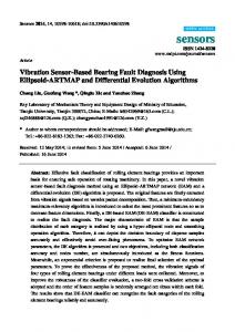
The unsupervised GRBM and the supervised GDBM were applied to learn the statistical features of the vibration signals. The statistical features represented by the unsupervised GRBM required an additional classifier for the pattern classification. Considering its excellent classification capability, the SVM was used as the classifier for the GRBM representations. For the GDBM, supervised deep learning as shown in Figure 3 was applied for the healthy condition pattern classification of the gearbox. 3.2. Experimental Procedure for Bearing Fault Diagnosis To further challenge the deep statistical feature learning for fault diagnosis, we also carried out bearing fault diagnosis experiments. The gear fault patterns (displayed in Table 1) occupied areas of great damage, which introduced greater changes in the vibration measurements [44]. Compared to the vibration signal of the gear fault, an incipient bearing fault often has a smaller damage surface and thus generates weak vibration changes [45]. As shown in Figure 5a, a rolling element bearing test rig was constructed in the Universidad Politécnica Salesiana of Ecuador to collect the vibration measurements for different healthy conditions. The test rig was driven by a motor (3~, 2.0 HP, Siemens) controlled by an inverter (VLT 1.5 kW, Danfoss). The rotating speed of the motor was monitored by a tachometer (VLS5/T/LSR optical sensor, Compact). A steel shaft (φ30 mm) was connected to the motor via a coupling. The two ends of the shaft were supported by two bearings (bearing 1 and bearing 2, 1207 EKTN9/C3, SKF, Goteborg, Sweden). An accelerometer (ICP 353C03, PCB) was mounted on the housing (SNL 507-606, SKF) of bearing 2 for measuring the vibration signals, which were collected by a data acquisition box (cDAQ-9234, NI) that communicated with a laptop (Pavilion g4-2055la, HP). Two flywheels were installed on the shaft as the load of the system. In addition to the normal bearings, as shown in Figure 5b, three different faulty bearings with an inner race fault, an outer race fault and a ball fault, were used in the experiments. Using combinations of bearings in different conditions, seven healthy condition patterns were set, as shown in Table 1. For each experiment with each pattern, there were respectively 0, 1 and 2 flywheels used as the load. For each pattern and load configuration, 48 signals were collected for 0.4096 s. Each experiment was repeated five times. This means that 5040 signals were finally obtained. The sampling frequency for the bearing fault diagnosis was also set at 10 kHz. Similar to the procedure described in the previous section, the statistical features were produced from the raw data of the bearing vibration signals. The unsupervised GRBM and the supervised GDBM

Sensors 2016, 16, 895

10 of 19

were again applied for the fault diagnosis of the bearing system. The results of all the experiments are Sensors 2016, 16, 895 10 of 19 detailed in the next section.

(a)

(a)

(b) Figure 5. Fault diagnosis configurations for the rolling element bearings: (a) experimental set-up; and (b) 3 different faulty bearings with an inner race fault (left), an outer race fault (middle) and a ball fault (right), respectively.

Similar to the procedure described in the previous section, the statistical features were produced from the raw data of the bearing vibration signals. The unsupervised GRBM and the supervised (b) GDBM were again applied for the fault diagnosis of the bearing system. The results of all the Figure 5. Fault diagnosis configurations for the rolling element bearings: (a) experimental set-up; and Figure 5. detailed Fault diagnosis for the rolling element bearings: (a) experimental set-up; and experiments are in theconfigurations next section. (b) 3 different faulty bearings with an inner race fault (left), an outer race fault (middle) and a ball

4.

(b) 3 different faulty bearings with an inner race fault (left), an outer race fault (middle) and a ball fault (right), respectively. respectively. Resultsfault and(right), Discussion

Similar to the procedure described in the previous section, the statistical features were produced

4. Results and Discussion from the raw data of Results the bearing vibration signals. The unsupervised GRBM and the supervised 4.1. Gearbox Fault Diagnosis

GDBM were again applied for the fault diagnosis of the bearing system. The results of all the

4.1. Gearbox Faultare Diagnosis experiments detailedResults in the next section.

Figure 6a,b plot the time domain waveform and statistical features for the first signal collected 6a,b plot the timesetup. domain waveform and statistical features for the the first signal frequency collected of from the Figure gearbox As the signal covered 0.4096 s with sampling 4. Results experimental and Discussion from the gearbox experimental setup. As the signal covered 0.4096 s with the sampling frequency 10 kHz, the length of the discrete time signal is 4096. For all the collected 3600 signals, their time of 10 4.1. kHz, the length of the discrete Gearbox Fault Diagnosis Results time signal is 4096. For all the collected 3600 signals, their time domain waveforms and statistical features are shown in Figure 6c,d, respectively. domain waveforms and statistical features are shown in Figure 6c,d, respectively.

Feature value

1

0

-0.5

-1 0

Feature value

0.5 Amplitude (V)

Amplitude (V)

Figure 6a,b plot the time domain waveform and statistical features for the first signal collected from1the gearbox experimental setup. As the signal covered 0.4096 s with the sampling frequency of 10 10 kHz, the length of the discrete time signal is 4096. For all the collected 3600 signals, their time 8 Figure 6c,d, respectively. domain waveforms and statistical features are shown in 0.5

0

0.05-0.5 0.1

-1 0

0.15

0.05

0.2 0.25 Time (S)

0.1 0.15 (a)

0.3

0.35

0.4

6 10

84 62

4

0

0 0.2 0.25 Time (S)

(a)

0.3

0.35

0.4

1

2

3

2

1

Figure 6. Cont.

2

3

4 5 6 7 8 Number of the statistical features

(b)

4 5 6 7 8 Number of the statistical features

(b)

9

9

Sensors 2016, 16, 895 Sensors 2016, 2016, 16, 16, 895 895

88

3000 3000 No.ofofthe thesignal signal No.

66

2000 2000 44

1000 1000

22

No.ofofthe thestatistical statisticalfeature feature No.

11 11 of of 19 19 30 30

99 88

25 25

77 66

20 20 15 15

55 44

10 10

33 22

55

11

00 00

0.1 0.1

0.2 0.2 Time Time (S) (S)

0.3 0.3

0.4 0.4

00

1000 1000

3000 2000 3000 2000 No. No. of of the the signal signal

(c) (c)

00

(d) (d)

Figure domain features for the gearbox fault diagnosis: (a) time domain waveform of first Figure 6. 6. Time Time fault diagnosis: (a) (a) time domain waveform of the the Figure 6. Timedomain domainfeatures featuresfor forthe thegearbox gearbox fault diagnosis: time domain waveform of first the signal; (b) time domain statistical features of the first signal; (c) time domain waveforms of the 3600 signal; (b) time domain statistical features of theoffirst (c) time domain waveforms of theof3600 first signal; (b) time domain statistical features the signal; first signal; (c) time domain waveforms the collected signals; and time domain statistical features of collected signals. collected signals; and (d) (d) domain statistical features of the theof3600 3600 collected signals. 3600 collected signals; andtime (d) time domain statistical features the 3600 collected signals.

Vibration Vibration signals signals were were then then transformed transformed into into the the frequency frequency domain. domain. The The frequency frequency domain domain Vibration signals were then transformed into the frequency domain. The frequency domain representation and statistical features for the first signal are shown in Figure 7a,b, respectively. representation and statistical features for the first signal are shown in Figure 7a,b, respectively. As As representation and statistical 10 features the for the first signal are shownininFigure Figure 7a,b, respectively. the the sampling sampling frequency frequency was was 10 kHz, kHz, the effective effective frequency frequency band band in Figure 7a 7a is is [0, [0, 5000] 5000] Hz. Hz. As the samplingare frequency was 10 kHz, the effectivewaveform. frequency band in Figurethere 7a is [0, only 5000] Hz. However, However, there there are only only 4096 4096 points points for for the the temporal temporal waveform. This This means means that that there are are only 2048 2048 However, there are only 4096 points for theHz. temporal waveform. This means thattheir therefrequency are only frequency points ranging between [0, 5000] For all the collected 3600 signals, frequency points ranging between [0, 5000] Hz. For all the collected 3600 signals, their frequency 2048 frequency points ranging between [0, 5000]are Hz. For allinthe collected 3600 signals, their frequency domain domain representations representations and and statistical statistical features features are shown shown in Figure Figure 7c,d, 7c,d, respectively. respectively. domain representations and statistical features are shown in Figure 7c,d, respectively. 30 30 25 25 value Featurevalue Feature

Amplitude(V) (V) Amplitude

40 40

30 30 20 20

20 20

15 15 10 10 55

10 10 00 00

1000 1000

2000 3000 2000 3000 Frequency Frequency (Hz) (Hz)

4000 4000

00 11

5000 5000

22

33

1400 1400 1200 1200

No.ofofthe thesignal signal No.

3000 3000

2000 2000

1000 1000 800 800

1000 1000

600 600 400 400 200 200

00

00

1000 1000

2000 4000 2000 3000 3000 4000 Frequezcy Frequezcy (hz) (hz)

(c) (c)

99

(b) (b)

5000 5000

No.ofofthe thefeature feature No.

(a) (a)

44 55 66 77 88 Number Number of of the the statistical statistical features features

99 88

5000 5000

77 66

4000 4000 3000 3000

55 44

2000 2000

33 22

1000 1000

11 00

1000 1000

2000 3000 2000 3000 No. No. of of the the signal signal

(d) (d)

Figure 7. gearbox fault diagnosis: frequency domain domain Figure Frequency domain domain features features for the gearbox Figure 7. 7. Frequency Frequency domain features for the gearbox fault fault diagnosis: diagnosis: (a) (a) frequency domain representation of the first signal; (b) frequency domain statistical features of the first signal; representation firstfirst signal; (b) frequency domaindomain statisticalstatistical features offeatures the first signal; frequency representationofofthethe signal; (b) frequency of the (c) first signal; (c) domain of the collected signals; (d) domain domain representations of all the collected 3600 and3600 (d) frequency domain statistical features (c) frequency frequency domain representations representations of all all thesignals; collected 3600 signals; and and (d) frequency frequency domain statistical features the of all the collected 3600 statistical features of of all allsignals. the collected collected 3600 3600 signals. signals.

For generating the time-frequency domain the WPT was applied to decompose For domain representations, representations, the the WPT WPT was was applied applied to to decompose decompose For generating generating the the time-frequency time-frequency domain representations, the raw data up to four levels. There are 2, 4, 8 and 16 nodes for each level. Put all the nodes together, the raw data up to four levels. There are 2, 4, 8 and 16 nodes for each level. Put all the nodes the raw data up to four levels. There are 2, 4, 8 and 16 nodes for each level. Put all the nodes together, together, the WPT presentation and statistical features are displayed in 8a,b, As the length the WPT WPT presentation presentation and and statistical statistical features features are are displayed displayed in in Figure Figure 8a,b, 8a,b, respectively. respectively. As As the the length length the Figure respectively.

Sensors 2016, 16, 895 Sensors 2016, 16, 895

12 of 19 12 of 19

of ofof data points forfor a node at the fourfour levels are 2052, 1030,1030, 519 of the the raw rawsignal signalisis4096 4096points, points,numbers numbers data points a node at the levels are 2052, and 264, 264, respectively. In this way,way, the number of data points as shown in Figure 8a is8a 16,600. For the 519 and respectively. In this the number of data points as shown in Figure is 16,600. For WPT, therethere are 30 nodes each each of which has nine This generates 270 features for thefor firstthe signal the WPT, are 30 nodes of which hasfeatures. nine features. This generates 270 features first as shown in Figure 8b. signal as shown in Figure 8b. All the the 3600 3600data datahave havebeen beendisordered disordered experiments. Among all 3600 the 3600 samples for forfor thethe experiments. Among all the samples for each each 2400 samples were random the training F. To represent the statistical data, data, 2400 samples were random chosenchosen as the as training datasetdataset F. To represent the statistical feature feature F, applied we firstthe applied the mon-layer GRBM with parameters as:the number ofin the set F, weset first mon-layer GRBM with parameters as: number of neurons theneurons hidden in the=hidden layer =of200, the learning epochs 150, therate initial learning rate = 0.001, layer 200, number the number learning of epochs = 150, the initial =learning = 0.001, its upper-bound = its upper-bound = 0.001,decay and the weight = 0.005. learning As unsupervised learning thehave GRBM 0.001, and the weight = 0.005. As decay unsupervised of the GRBM does of not the does not havefunction, the classification function, a multi-class classifier wasthe applied to obtain the classification a multi-class SVM classifier was SVM applied to obtain first fault diagnosis first fault model 1 peerfor model). The reasonthe formodel us to is implement theperformance model is to of show model (# 1diagnosis peer model). The(#reason us to implement to show the the the performance of theFor present deep learning. For # 1 peer the feature GRBM representation acts as the second present deep learning. # 1 peer model, the GRBM acts as model, the second tool feature representation toolby(statistical by Equation (7) is themeasurements. first one) for the vibration (statistical features given Equation features (7) is thegiven first one) for the vibration The outputs measurements. Thefed outputs of SVM the GRBM wereThe fedsupervised into the SVM classifier. The supervised GDBM of the GRBM were into the classifier. GDBM was subsequently applied for was subsequently for the same dataset of F with parameters as:hidden number of the neurons in the the same dataset Fapplied with parameters as: number the neurons in the layer 1 = 200, number of hidden layerin 1= 200, number of 2the neurons in the layer 2 =epochs 200, number of constituent the pretraining the neurons the hidden layer = 200, number of hidden the pretraining (for each and epochs (for each model) =epochs 150, number of the fine-tuning 150, its theupperinitial the model) = 150,constituent number ofand the the fine-tuning = 150, the initial learningepochs rate = = 0.001, bound =rate 0.001, and the weight decay==0.001, 0.005.and In this way, we obtained theInsecond fault learning = 0.001, its upper-bound the weight decay = 0.005. this way, wediagnosis obtained model (the fault proposed GDBM model). For comparison, SVM For classifiers for thethe original statistical the second diagnosis model (the proposed GDBMthe model). comparison, SVM classifiers features M(p,q),statistical and thefeatures combination M(p,q) and the GRBM representation were respectively for the original M(p,q),ofand the combination of M(p,q) and the GRBM representation developed as the third fault diagnosis model (#2 peer model) and(#2 thepeer fourth one (#3 All were respectively developed as the third fault diagnosis model model) andpeer the model). fourth one ® ® the peer algorithms realized using were Matlab . One using may note that .inOne thismay work wethat have (#3 model).were All the algorithms realized Matlab note innot thisemployed work we morenot “shallow” learning such as the decision tree, as thethe random forest, neural network. have employed more models “shallow” learning models such decision tree,and the the random forest, and Theneural reasonnetwork. is that the SVM has isbeen thehas prominent representative which outperformswhich most the The reason thatproven the SVM been proven the prominent representative of the “shallow” members.learning members. outperforms mostlearning of the “shallow” 1.5

12

10 8

Feature value

WPT coefficient

1 0.5

0

6 4 2

-0.5

0

-1 0

2000 4000 6000 8000 10000 12000 14000 16000 Number of points

0

50

(a)

(b) 25 0

10 5 0

2000

-5 -10

1000

No. of the feature

15 3000

No. of the signal

100 150 200 250 Number of the statistical features

250

200

200

150

150

100

100

50

50

-15 0

0

5000

10000 Data point

(c)

15000

0

0 0

1000

2000 3000 No. of the signal

(d)

Figure 8. 8. Time-frequency WPT representation of Figure Time-frequency domain domain features featuresfor forthe thegearbox gearboxfault faultdiagnosis: diagnosis:(a)(a) WPT representation thethe first signal; (c) time-frequency time-frequency of first signal;(b) (b)time-frequency time-frequencydomain domainstatistical statisticalfeatures featuresof ofthe the first first signal; signal; (c) domain representations of all the collected 3600 signals; and (d) time-frequency domain statistical domain representations of all the collected 3600 signals; and (d) time-frequency domain statistical features of all the collected 3600 signals. features of all the collected 3600 signals.

Sensors 2016, 16, 895

13 of 19

With the trained models, the remaining 1200 samples (in the time, frequency, and time-frequency domains, respectively) were used to test the classification performances, which are displayed in Table 2. From the diagnosis results shown in Table 2, it is clear that the classification rates for the time-frequency domain statistical features are higher (72.09% on average) than those for the time and frequency domains. This is due to the joint time and frequency representation of the WPT. When comparing the statistical features of the time and frequency domains, the time domain features are always the worst. Among all the models, deep statistical feature learning via the GDBM exhibits the best classification rate for the same data (62.58%, 91.75%, 95.17%, and 83.17% for the time, frequency, time-frequency domain statistical features, and the average, respectively). The best classification rate of 95.17% is seen with the GDBM model and time-frequency statistical features. Compared to supervised learning methods (e.g., the GDBM), the unsupervised GRBM displays the lowest classification rates (26.67%, 52.67%, 42.25%, and 41.33% for the time, frequency, time-frequency domain statistical features, and the average, respectively). Nevertheless, it should be noted that the GRBM used in this paper is an unsupervised algorithm, which shows that there is still some potential for fault diagnosis, if a fine-tuning procedure can be introduced for its learning process. As one of the most important “shallow” learning approaches, the SVM exhibited good classification results for the gearbox system. This result is similar to that of existing studies (e.g., [46]). When the GRBM representations are combined with the original statistical features M(p,q), a small increase in the classification rates can be seen (from 52.83% to 79.42% for the frequency domain, 69.50% to 78.42% for the time-frequency domain statistical features, and 61.05% to 64.56% on average). However, due to the “shallow” learning limit, it is very difficult to further improve the classification rate for the SVM. Our results indicate that deep statistical feature learning has the best performance for gearbox fault diagnosis. It should be noted that deep learning is much more time-consuming than classical learning methods. Table 2. Fault classification rates for the testing dataset (%), where N represents the device, d denotes the domain of the feature. Device (N)

Fault Diagnosis Model

Domain (d) #1 Peer

GDBM

#2 Peer

#3 Peer

Average a

Gearbox

Time domain Frequency domain Time-frequency domain Average b

26.08 52.67 45.25 41.33

62.58 91.75 95.17 83.17

60.83 52.83 69.50 61.05

35.83 79.42 78.42 64.56

46.33 69.17 72.09 62.53

Bearing

Time domain Frequency domain Time-frequency domain Average b

18.52 39.95 58.84 39.10

60.63 87.57 91.75 79.98

59.58 80.74 81.53 73.95

41.96 82.91 82.70 69.19

45.17 72.79 78.71 65.508

a

the average value of the left four models; b the average value of the above three domains.

4.2. Bearing Fault Diagnosis Results For the bearing fault diagnosis experiments, 5040 vibration signals and their statistical features in the time domain are plotted in Figure 9a,b. The Fourier transform were then used to generate the frequency data and their statistical features as shown in Figure 9c,d, respectively. The time-frequency representation produced by the 4-level WPT and their statistical features are shown in Figure 9e,f, respectively. Of the 5040 samples, 3150 of the bearing system vibration signals were randomly chosen as the training dataset F. Similar modeling procedures to the gearbox fault diagnosis were repeated to develop the bearing fault diagnosis models. For comparisons, the same parameters are used in this subsection for the four models (i.e., No. 1: GRBM, No. 2: GDBM, No. 3: SVM, and No. 4: GRBM-SVM). After obtaining the trained models, the remaining 1890 samples (in the time, frequency,

complex model with the largest number of parameters that must be estimated from the sample. It is an intrinsic drawback that “deeper” learning requires much more time than “shallow” learning does. As pointed out by LeCun et al. [48], the advent of fast graphics processing units (GPUs), which are convenient to program, allowed researchers to train deep networks 10 or 20 times faster. This Sensors 2016, 16, 895 14 of 19 indicates that parallel computation is helpful for reducing computation time. However, parallel computation is beyond the scope of this study. All the programs in this work were executed on a laptop. This resulted in muchwere moreapplied computation timeclassification (hour-level)performance for the presented GDBM than its and time-frequency domains) to test the for the bearing fault “shallow” counterparts (usually secondor minutelevel on a laptop). diagnosis. The results are displayed in Table 2. 9

3

4000

2 1

3000

0 2000

-1

6

0

0.1

0.2 Time (S)

0.3

15

5 4

10

3

5

2

-3 0

20

7

-2

1000

25

8 No. of the feature

No. of the signal

5000

1 0

0.4

0 1000

(a)

2000 3000 4000 No. of the signal

5000

(b)

5000

9

500

600

4000

400

3000

300

2000

200

1000

100

0

No. of the feature

No. of the signal

8

500

7 6

400

5

300

4 3

200

2

100

1 0

1000

Sensors 2016, 16, 895

2000 3000 4000 Frequency (Hz)

5000

0

1000

(c)

5000

15 of 19

(d)

5000

25 0

4

4000

2

3000 0 2000 -2 1000

No. of the feature

No. of the feature

2000 3000 4000 No. of the signal

300

200 150

200

100

100

50

-4 0

0

5000

10000 Data point

(e)

15000

0

0 0

1000

2000 3000 4000 No. of the signal

5000

(f)

Figure 9. 9. Bearing diagnosis experiments: experiments: (a) signals, (b) the time time domain domain Figure Bearing fault fault diagnosis (a) the the time time domain domain signals; (b) the statistical features, (c) the frequency domain representations, (d) the frequency domain statistical statistical features; (c) the frequency domain representations; (d) the frequency domain statistical features, (e) (e) the the WPT WPT results; results, and and (f) (f) the the time-frequency time-frequency domain domain statistical statisticalfeatures. features. features;

4.3. Remarks A comparison of the feature performances in the different domains in Table 2 suggests that the time–frequency domain features exhibit theshown best performances (58.84%, 91.75%, 81.53% andsee 82.70% Based on the fault diagnosis results as in the previous two subsections, one can that with the GRBM, GDBM, SVM and GRBM-SVM models, respectively), and thecomparing time domain features the deep statistical feature learning holds the best classification performance to the peer models. experiments, were veryfor aberrant valuesCompared (outliers) collected the have theDuring lowest the classification ratethere (45.17% onsome average all models). with the from gearbox experimental setups, because the for outliers are always unavoidable for more real applications. It is obvious fault diagnosis, the fault features the rolling element bearings are evident in the frequency that the outliers may leadhigh to deterioration of the fault diagnosis. However, we didcomparison not removeresults those domain, especially in the frequency resonance band [47]. However, the model outliers from the dataset, even if the removal of the outliers increasefault the classification rates. all for the bearing fault diagnosis are almost same as those for may the gearbox diagnosis. Among It should be noted thatstatistical the givenfeature parameters alsomodel play important roleshas to the GDBM model. As the peer models, the deep learning (the GDBM) best classification indicated by Cho et al. [35], the training procedure of the GDBM can easily runfor intothe problems without rate (60.63% for the time domain, 87.57% for the frequency domain, 91.75% time-frequency careful selection of the parameters. determining the network structure for different domain, and 79.98% onlearning average). This againUpon validates the effectiveness of deep statistical feature layers, therefore, the learning epochs for the pretraining and thethe fine-tuning will be related learning for fault diagnosis in rotating machinery. Nevertheless, improvement in directly fault diagnosis to the classification performance. In this subsection we will discuss the influence of the epochs for the pretraining and the fine-tuning procedure. We first adjusted the number of pretraining epochs (for the GRBMs and the presented model) with all the other parameters fixed. Figure 10a plots the change of the fault classification rates in response to the increase of the pretraining epochs for the WPT features. For the fault diagnosis of both the gearbox and the bearing systems, the number of

-2

No.

No.

2000 1000

100

100

50

-4 0 Sensors 2016, 16, 895 0 5000

10000 Data point

0

15000

0 0

1000

2000 3000 4000 No. of the signal

(e)

4.3.

500015 of 19

(f)

performance with deep learning is at the cost of complexity. The present GDBM is the most complex model with the largest number of parameters that must be estimated from the sample. It is an intrinsic Figure 9. Bearing fault diagnosis experiments: (a) the time domain signals, (b) the time domain drawback that “deeper” learning requires much more time than “shallow” learning does. As pointed statistical features, (c) the frequency domain representations, (d) the frequency domain statistical out by LeCun et al. [48], the advent of fast graphics processing units (GPUs), which are convenient to features, (e) the WPTresearchers results, and (f) the time-frequency features. program, allowed to train deep networks 10 ordomain 20 timesstatistical faster. This indicates that parallel computation is helpful for reducing computation time. However, parallel computation is beyond the scope of this study. All the programs in this work were executed on a laptop. This resulted in Remarks much more computation time (hour-level) for the presented GDBM than its “shallow” counterparts Based on the faultordiagnosis results as shown in the previous two subsections, one can see (usually secondminute- level on a laptop).

that the deep statistical feature learning holds the best classification performance comparing to the peer Remarks models.4.3. During the experiments, there were some very aberrant values (outliers) collected from the Based on the fault diagnosis results are as shown in the previous twofor subsections, one can see It that experimental setups, because the outliers always unavoidable real applications. is obvious the deep statistical feature learning holds the best classification performance comparing to the peer that the outliers may lead to deterioration of the fault diagnosis. However, we did not remove those models. During the experiments, there were some very aberrant values (outliers) collected from the outliers experimental from the dataset, even if the removal of the outliers may increase the classification rates. setups, because the outliers are always unavoidable for real applications. It is obvious It should noted that the given parameters also play important the GDBM model. As that thebe outliers may lead to deterioration of the fault diagnosis. However, roles we didto not remove those indicated by Cho etthe al. dataset, [35], the training procedure the GDBM can easily run into problems without outliers from even if the removal of theof outliers may increase the classification rates. It should be noted that the given parameters play important roles to thestructure GDBM model. careful selection of the learning parameters. Upon also determining the network for different As indicated by Cho et al. [35], the training procedure of the GDBM can easily run into problems layers, therefore, the learning epochs for the pretraining and the fine-tuning will be directly related without careful selection of the learning parameters. Upon determining the network structure for to the classification performance. In this subsection we will discuss the influence of the epochs for the different layers, therefore, the learning epochs for the pretraining and the fine-tuning will be directly pretraining and theclassification fine-tuning procedure. first adjusted number of pretraining epochs (for related to the performance. In We this subsection we willthe discuss the influence of the epochs the GRBMs and the presented with all the We other fixed. Figure 10a plots the change for the pretraining and the model) fine-tuning procedure. firstparameters adjusted the number of pretraining epochs (for the GRBMs and the presented model) with all the other parameters fixed. Figure 10a plots the of the fault classification rates in response to the increase of the pretraining epochs for the WPT of thefault fault diagnosis classificationof rates in response to the increase of the pretraining epochsthe for the features.change For the both the gearbox and the bearing systems, number of WPT features. For the fault diagnosis of both the gearbox and the bearing systems, the number of pretraining epochs does not influence the classification very much. This means that even for a small pretraining epochs does not influence the classification very much. This means that even for a small numbernumber (e.g., 10) of10) theofepochs, thethe pretraining canachieve achieve good effect. (e.g., the epochs, pretraining can good effect. 100

Classification rate (%)

Classification rate (%)

100 90 80

Gearbox Bearings

70 60

Gearbox

80

Bearings 70 60 50

50 40

90

0

50

100 150 Pretraining epochs

(a)

200

250

40

0

50

100 150 Fine-tuning epochs

200

250

(b)

Figure 10. Relationship between classification rate thethe number of theofmodeling epochs: epochs: Figure 10. Relationship between thetheclassification rateand and number the modeling (a) classification v.s. pretrainingepochs; epochs; and and (b) ratesrates vs. fine-tuning epochs of the (a) classification rates rates v.s. pretraining (b)classification classification vs. fine-tuning epochs of the time-frequency domain GDBM models. time-frequency domain GDBM models.

The pretraining epochs were subsequently set at 150 to adjust the number of the fine-tuning epochs

The pretraining epochs were subsequently set at 150 to adjust the number of the fine-tuning between 10 and 250. The fault classification rates for the two mechanical systems were displayed in epochs Figure between and 250. The fault classification rates for the two mechanical systems were 10b. 10 With the increase of the fine-tuning epochs, the classification rates for both experiments displayed in Figure 10b. With thegearbox increase of the fine-tuning the classification improve accordingly. For the diagnosis experiments, epochs, the improvement goes slowlyrates after for both 125 epochs. As foraccordingly. the bearing systems, the classification rate increases still evidently before 200 epochs. experiments improve For the gearbox diagnosis experiments, the improvement goes

Sensors 2016, 16, 895

16 of 19

slowly after 125 epochs. As for the bearing systems, the classification rate increases still 16 evidently Sensors 2016, 16, 895 of 19 before 200 epochs. Figure 10a,b prove that the deep statistical feature learning using the GDBM is not very sensitive to the learning parameters. Even though, a careful selection of the model parameters Figure 10a,b prove that the deep statistical feature learning using the GDBM is not very sensitive to will be helpful in improving the fault pattern classification for the rotating machinery. This means the learning parameters. Even though, a careful selection of the model parameters will be helpful in that improving the proposed method hasclassification an essential potentialThis formeans the fault diagnosis of the the fault pattern forimprovement the rotating machinery. that the proposed rotating machinery. method has an essential improvement potential for the fault diagnosis of the rotating machinery. Figure 11a–c plots thethe comparisons faultpatterns patterns and classified patterns Figure 11a–c plots comparisonsbetween between the the real real fault and thethe classified patterns for for the bearing faultfault diagnosis in in thethe time, thetime-frequency time-frequency domains, respectively. the bearing diagnosis time,the thefrequency frequency and and the domains, respectively. It is shown that some signals are correctly classified by the proposed method in some domains, but but It is shown that some signals are correctly classified by the proposed method in some domains, are misclassified in other domains.Let’s Let’stake take 10 10 vibration of the bearing faultfault are misclassified in other domains. vibrationsignals signals(#286~#295) (#286~#295) of the bearing diagnosis as an example. The time domain diagnosis misclassified #295 signal, while both the frequency diagnosis as an example. The time domain diagnosis misclassified #295 signal, while both the domain and the time-frequency domain obtained right classification. The frequency domain diagnosis frequency domain and the time-frequency domain obtained right classification. The frequency misclassified #290 signal, but all the other two domains are correct. The time-frequency domain domain diagnosis misclassified #290 signal, but all the other two domains are correct. The timediagnosis misclassified #286 signal, while all the rest domains are right. If one considers the three frequency domain diagnosis misclassified #286 signal, while all the rest domains are right. If one domains simultaneously, therefore, all the 10 vibration signals (#286~#295) can be right diagnosed. considers the three simultaneously, therefore, all may the 10 vibrationbetter signals (#286~#295) can be This shows thatdomains the combination of the diagnosis results contribute classification rates. rightThough diagnosed. shows the combination of encourages the diagnosis results may contribute better out ofThis our scope in that this paper, this discussion us that further potentials can be classification rates. Though out of our scope in this paper, this discussion encourages us that further explored for the proposed fault diagnosis approach. potentials can be explored for the proposed fault diagnosis approach. 286 286~295

290

6 5 4

7

292 294 Real pattern Diagnosed

286~295

Pattern No.

7 6 5 4 3 2 1

7

Pattern No.

288

3

286

288

290

6 5

7

4 3

6

2

5

1

292 294 Real pattern Diagnosed

4 3 2

2

1

1 0

0

500

1000 No. of the signal

500

1500

(a)

1000 No. of the signal

1500

(b) 286

288

290

7 6

286~295

292 294 Real pattern Diagnosed

5 6

4 3

5

1

Pattern No.

7

2

4 3 2 1 0

500

1000 No. of the signal

1500

(c) Figure 11. Bearing fault diagnosis results domains:(a) (a)the thetime time domain; frequency Figure 11. Bearing fault diagnosis resultsinindifferent different domains: domain; (b) (b) the the frequency domain; (c) the time-frequencydomain. domain. domain; andand (c) the time-frequency

5. Conclusions 5. Conclusions In paper, this paper, a deep statistical featurelearning learning for for vibration hashas been proposed to to In this a deep statistical feature vibrationmeasurement measurement been proposed diagnose fault patterns in rotating machinery. The statistical feature set was first extracted from the diagnose fault patterns in rotating machinery. The statistical feature set was first extracted from the time, frequency, and time-frequency domains of the vibration signals. The real-valued RBMs were then stacked to develop a GDBM to accommodate statistical feature learning. Two typical rotating machinery systems (a gearbox and bearing test rigs), were constructed to validate the proposed approach, which was used for fault classification in the three-domain feature sets. The results show

Sensors 2016, 16, 895

17 of 19

time, frequency, and time-frequency domains of the vibration signals. The real-valued RBMs were then stacked to develop a GDBM to accommodate statistical feature learning. Two typical rotating machinery systems (a gearbox and bearing test rigs), were constructed to validate the proposed approach, which was used for fault classification in the three-domain feature sets. The results show that deep statistical feature learning is capable of classifying fault patterns at higher rates than other models. Compared with the unsupervised GRBM, the SVM and the combined SVM and GRBM models, the deep statistical feature learning by the GDBM consistently had clearly better performances. This means that deep learning with statistical feature representation is a feasible update of conventional methods. The results also reveal that the statistical features in the time, frequency and time–frequency domains have different representation capabilities for fault patterns. Our further work will focus on optimizing the statistical features in different domains for different diagnostic applications. Acknowledgments: This work is supported in part by the Secretariat for Higher Education, Science, Technology and Innovation of the Republic of Ecuador (GIDTEC project No. 009-004-2015-07-16), the National Natural Science Foundation of China (Grant No. 51375517), and the Project of Chongqing Science & Technology Commission (Grant No. cstc2014gjhz70002). The valuable comments and suggestions from the two anonymous reviewers are very much appreciated. Author Contributions: Chuan Li designed the experiments and wrote the paper; Vinicio Sanchez contributed experimental set-up and materials; Grover Zurita and Mariela Cerrada analyzed the data; Diego Cabrera performed the experiments. Conflicts of Interest: The authors declare no conflict of interest.

References 1. 2. 3. 4. 5.

6.

7.

8.

9.

10.

11. 12.

Lei, Y.; Lin, J.; Zuo, M.J.; He, Z. Condition monitoring and fault diagnosis of planetary gearboxes: A review. Measurement 2014, 48, 292–305. [CrossRef] Li, C.; Liang, M. Time-frequency signal analysis for gearbox fault diagnosis using a generalized synchrosqueezing transform. Mech. Syst. Sig. Process. 2012, 26, 205–217. [CrossRef] Batista, L.; Badri, B.; Sabourin, R.; Thomas, M. A classifier fusion system for bearing fault diagnosis. Expert Syst. Appl. 2013, 40, 6788–6797. [CrossRef] Li, C.; Liang, M.; Wang, T. Criterion fusion for spectral segmentation and its application to optimal demodulation of bearing vibration signals. Mech. Syst. Sig. Process. 2015, 64–65, 132–148. [CrossRef] Gao, Z.; Cecati, C.; Ding, S.X. A survey of fault diagnosis and fault-tolerant techniques—Part I: Fault diagnosis with model-based and signal-based approaches. IEEE Trans. Ind. Electron. 2015, 62, 3757–3767. [CrossRef] Gao, Z.; Cecati, C.; Ding, S.X. A survey of fault diagnosis and fault-tolerant techniques—Part II: Fault diagnosis with knowledge-based and hybrid/active-based approaches. IEEE Trans. Ind. Electron. 2015, 62, 3768–3774. [CrossRef] Qin, Q.; Jiang, Z.N.; Feng, K.; He, W. A novel scheme for fault detection of reciprocating compressor valves based on basis pursuit wave matching and support vector machine. Measurement 2010, 45, 897–908. [CrossRef] Wong, W.K.; Loo, C.K.; Lim, W.S.; Tan, P.N. Thermal condition monitoring system using log-polar mapping, quaternion correlation and max-product fuzzy neural network classification. Neurocomputing 2010, 74, 164–177. [CrossRef] Arumugam, V.; Sidharth, A.A.P.; Santulli, C. Failure modes characterization of impacted carbon fibre reinforced plastics laminates under compression loading using acoustic emission. J. Compos. Mater. 2014, 48, 3457–3468. [CrossRef] Li, C.; Peng, J.; Liang, M. Enhancement of the wear particle monitoring capability of oil debris sensors using a maximal overlap discrete wavelet transform with optimal decomposition depth. Sensors 2014, 14, 6207–6228. [CrossRef] [PubMed] Raad, A.; Antoni, J.; Sidahmed, M. Indicators of cyclostationarity: Theory and application to gear fault monitoring. Mech. Syst. Sig. Process. 2008, 22, 574–587. [CrossRef] Bartelmus, W.; Zimroz, R. A new feature for monitoring the condition of gearboxes in non-stationary operating conditions. Mech. Syst. Sig. Process. 2009, 23, 1528–1534. [CrossRef]

Sensors 2016, 16, 895

13. 14. 15. 16. 17.

18. 19. 20.

21.

22. 23.

24. 25. 26. 27.

28. 29. 30.

31. 32.

33. 34.

18 of 19

Randall, R.B.; Antoni, J. Rolling element bearing diagnostics—A tutorial. Mech. Syst. Sig. Process. 2011, 25, 485–520. [CrossRef] Li, C.; Liang, M. Continuous-scale mathematical morphology-based optimal scale band demodulation of impulsive feature for bearing defect diagnosis. J. Sound Vib. 2012, 331, 5864–5879. [CrossRef] Zuo, M.J.; Lin, J.; Fan, X. Feature separation using ICA for a one-dimensional time series and its application in fault detection. J. Sound Vib. 2005, 287, 614–624. [CrossRef] Kumar, R.; Singh, M. Outer race defect width measurement in taper roller bearing using discrete wavelet transform of vibration signal. Measurement 2013, 46, 537–545. [CrossRef] Shen, C.; Wang, D.; Kong, F.; Tse, P.W. Fault diagnosis of rotating machinery based on the statistical parameters of wavelet packet paving and a generic support vector regressive classifier. Measurement 2013, 46, 1551–1564. [CrossRef] Cao, H.; Chen, X.; Zi, Y.; Ding, F.; Chen, H.; Tan, J.; He, Z. End milling tool breakage detection using lifting scheme and Mahalanobis distance. Int. J. Mach. Tools Manuf. 2008, 48, 141–151. [CrossRef] Wang, D.; Tse, P.W.; Guo, W.; Miao, Q. Support vector data description for fusion of multiple health indicators for enhancing gearbox fault diagnosis and prognosis. Meas. Sci. Technol. 2011, 22, 025102. [CrossRef] Li, C.; Cabrera, D.; Valente de Oliveira, J.; Sanchez, R.V.; Cerrada, M.; Zurita, G. Extracting repetitive transients for rotating machinery diagnosis using multiscale clustered grey infogram. Mech. Syst. Sig. Process. 2016, 76–77, 157–173. [CrossRef] Li, C.; Sanchez, V.; Zurita, G.; Lozada, M.C.; Cabrera, D. Rolling element bearing defect detection using the generalized synchrosqueezing transform guided by time-frequency ridge enhancement. ISA Trans. 2016, 60, 274–284. [CrossRef] [PubMed] Lei, Y.; Kong, D.; Lin, J.; Zuo, M.J. Fault detection of planetary gearboxes using new diagnostic parameters. Meas. Sci. Technol. 2012, 23, 055605. [CrossRef] Cerrada, M.; Sánchez, R.V.; Cabrera, D.; Zurita, G.; Li, C. Multi-stage feature selection by using genetic algorithms for fault diagnosis in gearboxes based on vibration signal. Sensors 2015, 15, 23903–23926. [CrossRef] [PubMed] Chen, F.; Tang, B.; Chen, R. A novel fault diagnosis model for gearbox based on wavelet support vector machine with immune genetic algorithm. Measurement 2013, 46, 220–232. [CrossRef] Zhao, M.; Jin, X.; Zhang, Z.; Li, B. Fault diagnosis of rolling element bearings via discriminative subspace learning: visualization and classification. Expert Syst. Appl. 2014, 41, 3391–3401. [CrossRef] Tayarani-Bathaie, S.S.; Vanini, Z.N.S.; Khorasani, K. Dynamic neural network-based fault diagnosis of gas turbine engines. Neurocomputing 2014, 125, 153–165. [CrossRef] Ali, J.B.; Fnaiech, N.; Saidi, L.; Chebel-Morello, B.; Fnaiech, F. Application of empirical mode decomposition and artificial neural network for automatic bearing fault diagnosis based on vibration signals. Appl. Acoust. 2015, 89, 16–27. Tamilselvan, P.; Wang, P. Failure diagnosis using deep belief learning based health state classification. Reliab. Eng. Syst. Saf. 2013, 115, 124–135. [CrossRef] Tran, V.T.; Thobiani, F.A.; Ball, A. An approach to fault diagnosis of reciprocating compressor valves using Teager-Kaiser energy operator and deep belief networks. Expert Syst. Appl. 2014, 41, 4113–4122. [CrossRef] Wang, Y.; Xu, G.; Liang, L.; Jiang, K. Detection of weak transient signals based on wavelet packet transform and manifold learning for rolling element bearing fault diagnosis. Mech. Syst. Sig. Process. 2015, 54–55, 259–276. [CrossRef] Randall, R.B. Vibration-Based Condition Monitoring: Industrial, Aerospace and Automotive Applications; John Wiley & Sons: Chichester, UK, 2011. Li, C.; Sanchez, R.V.; Zurita, G.; Cerrada, M.; Cabrera, D.; Vásquez, R.E. Multimodal deep support vector classification with homologous features and its application to gearbox fault diagnosis. Neurocomputing 2015, 168, 119–127. [CrossRef] Hinton, G.E.; Salakhutdinov, R.R. Reducing the dimensionality of data with neural networks. Science 2006, 313, 504–507. [CrossRef] [PubMed] Hjelma, D.; Calhouna, V.; Salakhutdinov, R.; Allena, E.; Adali, T.; Plisa, S. Restricted Boltzmann machines for neuroimaging: An application in identifying intrinsic networks. Neuroimage 2014, 96, 245–260. [CrossRef] [PubMed]

Sensors 2016, 16, 895

35.

36. 37. 38. 39. 40. 41. 42. 43. 44. 45. 46. 47. 48.

19 of 19

Cho, K.H.; Ilin, A.; Raiko, T. Improved Learning of Gaussian-Bernoulli Restricted Boltzmann Machines. In Artificial Neural Networks and Machine Learning—ICANN 2011; Springer Berlin Heidelberg: Berlin, Germany, 2011; Volume 6791, pp. 10–17. Salakhutdinov, R. Learning Deep Generative Models. Ph.D. Thesis, University of Toronto, Toronto, ON, Canada, 2009. Hastie, T.; Tibshirani, R. Classification by Pairwise Coupling. In Advances in Neural Information Processing Systems 10; MIT Press: Cambridge, MA, USA, 1998. Cho, K.H.; Raiko, T.; Ilin, A. Gaussian-Bernoulli deep Boltzmann machine. In Proceedings of the 2013 International Joint Conference on Neural Networks, Dallas, TX, USA, 4–9 August 2013; pp. 1–7. Schmidhuber, J. Deep learning in neural networks: An overview. Neural Netw. 2015, 61, 85–117. [CrossRef] [PubMed] Salakhutdinov, R. Learning in Markov Random Fields Using Tempered Transitions. In Advances in Neural Information Processing Systems 22; MIT Press: Cambridge, MA, USA, 2009; pp. 1598–1606. Bishop, C.M. Neural Networks for Pattern Recognition; Clarendon Press: Oxford, UK, 1996. Nabney, I.T. NETLAB: Algorithms for Pattern Recognition; Springer-Verlag: London, UK, 2001. Hinton, G.E.; Osindero, S.; The, Y.W. A fast learning algorithm for deep belief nets. Neural Comput. 2006, 18, 1527–1554. [CrossRef] [PubMed] Khomfoi, S.; Tolbert, L.M. Fault diagnostic system for a multilevel inverter using a neural network. IEEE Trans. Power Electron. 2007, 22, 1062–1069. [CrossRef] Bartkowiak, A.; Zimroz, R. Outliers analysis and one class classification approach for planetary gearbox diagnosis. J. Phys. Conf. Ser. 2011, 305, 012031. [CrossRef] Souza, D.L.; Granzotto, M.H.; Almeida, G.M.; Oliveira-Lopes, L.C. Fault detection and diagnosis using support vector machines—A SVC and SVR comparison. J. Saf. Eng. 2014, 3, 18–29. [CrossRef] Hou, S.; Li, Y.; Wang, Z. A resonance demodulation method based on harmonic wavelet transform for rolling bearing fault diagnosis. Struct. Health Monit. 2010, 9, 297–308. LeCun, Y.; Bengio, Y.; Hinton, G.E. Deep learning. Nature 2015, 521, 436–444. [CrossRef] [PubMed] © 2016 by the authors; licensee MDPI, Basel, Switzerland. This article is an open access article distributed under the terms and conditions of the Creative Commons Attribution (CC-BY) license (http://creativecommons.org/licenses/by/4.0/).