Fault-Tolerant Earliest-Deadline-First Scheduling Algorithm - CiteSeerX

Fault-Tolerant Earliest-Deadline-First Scheduling Algorithm∗ Hakem Beitollahi1 [email protected] 1 2

Seyed Ghassem Miremadi2 [email protected]

Katholieke Universiteit Leuven, Electrical Engineering, Kasteelpark Arenberg 10, Leuven, Belgium Sharif University of Technology, Computer Engineering Department, Azadi Ave., Tehran, Iran

Abstract The general approach to fault tolerance in uniprocessor systems is to maintain enough time redundancy in the schedule so that any task instance can be re-executed in presence of faults during the execution. In this paper a scheme is presented to add enough and efficient time redundancy to the Earliest-Deadline-First (EDF) scheduling policy for periodic real-time tasks. This scheme can be used to tolerate transient faults during the execution of tasks. We describe a recovery scheme which can be used to re-execute tasks in the event of transient faults and discuss conditions that must be met by any such recovery scheme. For performance evaluation of this idea a tool is developed.

Keywords: Time-redundancy, real-time scheduling, fault-tolerance, uniprocessor embedded systems, earliestdeadline-first.

1. Introduction Embedded systems account for major part of critical application (space, aeronautics, nuclear…) as well as public domain applications (automotive, consumer electronic, etc.). The correctness of real-time embedded systems depends not only on the results of computations, but also on the time instants at which these results become available [1, 18]. One important issue in real-time embedded systems is the scheduling of tasks in these systems. Modern realtime scheduling research has mostly concentrated on generating efficient algorithms for guaranteeing that tasks meet their deadlines without considering faults. Several studies in the last three decades have concluded that transient faults are significantly more frequent than permanent faults [3, 4, 5, 8, 19]. In [19], measurement showed that transient faults are 30 times more frequent than permanent faults, while in [8], 83% of ∗

Geert Deconinck1 [email protected]

1-4244-0910-1/07/$20.00 ©2007 IEEE

all faults were determined to be transient or intermittent. Due to the high occurrence of transient faults in some applications, and because hardware redundancy can be used to tolerate permanent faults in embedded real-time systems [12, 14], we consider only the problem of transient and intermittent faults in this paper. Transient faults in real-time systems are generally tolerated using time redundancy, which involves the retry or re-execution of any task running during the occurrence of transient faults [6, 7, 9, 13, 16]. Moreover, this is a relatively inexpensive method of providing faulttolerance in real-time embedded systems. Several studies have done for using time redundancy in embedded realtime systems for tolerating faults. Pandya and Malek in [15] have used time redundancy for tolerating a single fault. In the event of faults, all unfinished tasks are reexecuted. In [16,17], authors have presented static and dynamic allocation strategies to provide fault-tolerance. Two algorithms have proposed to reserve time for the recovery of periodic real-time tasks on a uniprocessor [17]. In [2] authors have provided exact schedulability tests for fault-tolerant task sets. In their paper, time redundancy has employed to provide a predictable performance in the presence of failures. However no study has done about adding appropriate and efficient time redundancy into the schedule, which is the main contribution of this paper. In recent years, Earliest- Deadline-First (EDF) scheduling policy has been used to schedule real-time tasks in variety critical applications. However, EDF does not provide mechanisms for managing time redundancy, so that real-time tasks will complete within their deadlines even in the presence of faults. The goal of this paper is to add appropriate and efficient time redundancy to the EDF scheduling policy for schedule periodic and preemptive tasks. It is clear that more tasks are scheduled if less time redundancy is added. However in spite of this advantage, less number of tasks can be recovered (more tasks are missed their deadline). In contrast, if more time

redundancy is added into the schedule, fewer tasks are lost while less number of tasks can be scheduled. In fact for any pair of average task utilization and mean time to failure (α, MTTF) the efficient time redundancy is added to the schedule. An event driven simulator is designed and implemented for performance evaluation. Moreover, this scheme can be applied to any non-fault-tolerant scheduling policy for preemptive and periodic tasks (e.g., Rate-Monotonic (RM) scheduling policy). The rest of the paper is organized as follows: section 2 describes the task, system and faults model. Section 3 discusses adding time redundancy into the schedule. In section 4, we calculate efficient time redundancy for the EDF policy. Section 5 discusses our tool. We present simulation results in section 6 and followed by the conclusion in section 7.

2. Task, System and Faults Model Tasks are periodic and preemptive. The tasks are eligible for execution at the beginning of the period, and have to complete before the end of the period. A set of n tasks Σ = {τ 1 ,τ 2 ,...,τ n } are given with τ i = (ci , ri , di , Ti ) for i = 1,2,..., n where c i , ri , di and Ti are the computation time, release time, deadline and period of task τ i , respectively. The tasks are independent, that is, have no precedence constraints. The utilization u i of τ i is c i / Ti . Only uniprocessor systems are considered. The total utilization of the system is the fraction of processor time spent in the execution of the task set and is equal to U=

∑

n i =1

u i . The cost of preemption is assumed to be

negligible. Faults are assumed to be transient or intermittent. Only single task is affected by fault and so faults can be tolerated by re-executing. Fault-detection mechanism such as acceptance test is used to detect faults [10].

3. Fault-Tolerance by Using Time redundancy The general approach to fault-tolerance in uniprocessor systems is to make sure there is enough slack in the schedule to allow for re-executing of any task instance, if a fault occurs during its execution [13]. Tasks are executed following the usual EDF scheme if no faults occur (the slack is not used). However, when a fault occurs in a task, a recovery scheme is used to re-execute that task. In the EDF policy with utilization bound less than 100%, there is a natural amount of slack in uniprocessor. But this natural slack does not enough for re-executing faulty

tasks. To have one efficient fault-tolerant mechanism in the schedule it is necessary that additional slack time is added to the schedule. The insertion of slack and recovery mechanism is called the FT scheme. The recovery mechanism ensures that the reserved slack can be used for task re-executing before its deadline, without causing other tasks to miss deadlines. When fault is detected at the end of some task τ r , the system goes into recovery mode. In this mode, τ r will re-execute at its own priority. During recovery mode, any instance of a task that has a priority than that of τ r and a deadline greater than d r will be delayed until recovery is complete. The added slack is distributed throughout the schedule such that the amount of slack available over an interval of time (L) is proportional to the length of the interval (enough to enable the re-execution of any task). The ratio of slack S available over an interval of time L is thus constant and can be imagined to be the utilization of a backup task B, where S/L is the backup utilization. Formally, if the backup utilization is U B , and the backup time (slack time) available during an interval L is denoted by B L , then BL = U B L (3.1) One important issue here is calculated schedulability bound for fault-tolerant EDF policy. Liu and Layland in [11] have shown that, for a non-fault-tolerant EDF policy, any set of n tasks with a total utilization below than one is schedulable on uniprocessor system. On other words scheduling of tasks feasible if and only if U =

∑

n u i =1 i

≤ 1 . However in fault-

tolerant EDF with additional slack time the schedulability bound must be less than above bound. A straightforward way of computing a shcedulability bound for fault-tolerant EDF scheduling policy would be to decrease the bound by U B , i.e., U FT − EDF = U LL − U B , here Liu and Layland bound in [11] is denoted by U LL . So the schedulability bound for fault-tolerant EDF is 1 − U B . Utilization _ bound FT − EDF = 1 − U B (3.2)

3.1. Conditions for Recovery:

A recovery scheme that ensures the re-execution of any task after a fault has been detected must satisfy the following conditions:

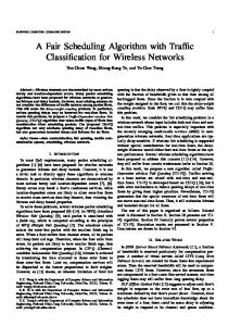
τ 11

0

τ 21

1

2

τ 11

0

3

τ 12 4

2

3

4

6

7

8

9

τ 13 10

11

12

13

14

12

13

14

13

14

(a)

fault

τ 21

1

5

τ 22

τ 12 5

τ 22

6

7

8

9

τ 13 10

11

(b) τ 11

0

τ 21

1

2

3

' τ 12

τ 12 4

5

6

7

8

τ 22 9

10

τ 13 11

12

(c) Figure 1. (a) tasks are scheduled in not present faults, (b) τ 12 has encountered with a fault , (c) the recover scheme has been called and τ 12 has been re-executed using time-redundancy

[C1]: There should be sufficient slack for every instance of each task to re-execute. [C2]: When a task re-executes, it should not cause any other task to miss its deadline. [C1] ensures the availability of sufficient slack for a task to re-execute, and [C2] ensures that all tasks meet their deadlines even when a high priority task needs to re-execute. Example: consider two tasks with c1 = 2, T1 = d1 = 5, c2 = 2, T2 = d 2 = 8 . The two 2 / 5 = 0.4 and utilizations are 2 / 8 = 0.25 respectively. Assuming that backup utilization is 0.2, i.e., U B = 0.2 . (3.2), gives us a bound of 0.8 while the sum of utilizations of the task is 0.65. Since U =

∑

n

u i =1 i

= 0.65 ≤ U FT − EDF = 0.8 ,

the tasks are schedulable. In figure 1.a no fault has occurred while the tasks are executed. In figure 1.b a fault has occurred when τ 12 ( τ 12 denotes the second period of τ 1 ) was being executed and has been detected at time 7, then recovery scheme has been called, i.e., new copy of τ 1 has been added to the schedule (figure 1.c), and has been completed using the slack time ( time redundancy).

4. Determining Efficient Value of Time Redundancy

Increasing the value of time redundancy has a considerable impact on the efficiency of scheduling and recovering tasks. In this section we determine appropriate and efficient value of time redundancy in the system for any pair of average task utilization (α) and mean time to fault (MTTF), i.e., any pair of (α, MTTF). To facilitate the discussion, the following variables are defined: • U B : the backup utilization of the system.

• • •

MTTF: the mean time to failure of the system. α: the average task utilization. Schedulability_value: the number of tasks that can be scheduled. • Lost_tasks_value: the number of task instances lost as a result of faults. • γ: the weight of Lost_tasks_value, which indicate the importance of Lost_tasks_value. • δ: the weight of Schedulability_value, which indicate the importance of Schedulability_value. In order to obtain an efficient value of time redundancy, we need only to obtain an appropriate value of U B . So the main goal of this section is to determine efficient value of U B for any pair of (α, MTTF). To solve the problem, we define the Gain variable that depends on Schedulability_value and Lost_tasks_value, and can be calculated using the following equation:

Gain = δ × Schedulability _ value − γ × Lost _ tasks _ value (4.1) In systems where the cost of losing a task instance is negligible, the value of γ is 0. For these systems, the

Gain variable only depends on how many tasks are scheduled, so the value of δ is considered to be high. On the other hand, when the gain of losing a task instance is high, the value of γ is much higher than the value of δ. In this case both value of γ and δ are important and must be determined correctly. In the case of the systems that the Schedulabilty_value as important as Lost_tasks_value, it is better to determine an equal value for δ and γ, i.e., γ = δ = 1. The ultimate goal of the system is to maximize Schedulabilty_value and to minimize Lost_tasks_value. In other words, the Gain variable should to be maximized. If chart of the Gain variable is plotted for different values of U B , MTTF, and α, we get the desired point where the Gain is maximized. Based on this point, the appropriate value of U B is determined. For example, if the task set has α of 10% while MTTF is 10 and γ = δ = 1 , then the value of U B , for which the Gain variable is maximized, is 15%. Such graphs can be generated for any known task set, and using fault injection, the appropriate value of U B can be determined. In the simulation results section for different cases, the value of U B is determined.

5. The Tool Our idea has been evaluated by a simulator that has been written in the C++ programming language. An eventdriven simulator is designed and implemented. A queue of events is maintained by the simulator and the events are handled according to their order. The simulator is sufficiently modular that different modules can be plugged in for various events to simulate a new scheduling, recovery or fault-tolerance policy. The simulation works as follows: •

Scheduling of tasks: The Earliest-Deadline-First (EDF) scheduling policy is used to schedule tasks. • Fault injection: Faults are injected into the schedule while tasks are running. Faults are generated based on a value of MTTF specified by the user. • Fault recovery: The recovery scheme used for tolerating transient faults. The following events are used to trigger an action: • Task arrival: The task is scheduled in the system. • Task begin: This is a time at which the task starts running. • Task end: This is the event when a task finishes running. A flag is checked to determine if faults have occurred during the execution of this task. If faults have occurred, then a recovery function is called.

•

Injected fault: A flag is raised to indicate that a fault has occurred. The pseudo code of the simulator looks as following: Function FT-EDF ( task set Σ, Start_time, End_time) /* task set Σ is input */ /* = {τ 1 ,τ 2 ,...,τ n } and τ i = (ci , ri , di , Ti ) */

∑

/* Start_time: indicate the start time of simulation. */ /* End_time: indicate the end time of simulation. */ Generate_Tasks( U B , α ); Generate_faults(end_time, MTTF); Get_nexet_event(); time_current = Start_time. /* time_current : indicate the current time in the simulator*/ While ( time _ current ≤ End _ time ) Begin Case ( next_event ): Begin TASK ARRIVE: schedule_task_with_EDF_policy(); TASK BEGIN : task_status = RUNNING; TASK END : If ( fault_occurred== TRUE) Then Fault_recovery(); FAULT : fault_occured = TRUE; END Case; Display_queue(); Increment time_current; Get_next_event(); END While; Analysis (); END Function FT-EDF

6. Simulation Results In this section, we present simulation results to determine efficient value of U B for any pair of average task utilization and mean time to failure (α, MTTF). A set of periodic tasks is generated for every run of the simulation. On each task set, Ti is generated following a uniform distribution with 10 ≤ Ti ≤ 100 and ci is generated following a uniform distribution in the range 0 < c i ≤ 2αTi , where α is average task utilization. For each result, the simulation was run 1000 times and the individual values were averaged. Each simulation was run for 10,000 time units First, the effect of U B on Schedulability_value is studied. As U B increased, the Schedulability_value is decreased. Figure 2 shows the Schedulability_value of the task sets using different values of α.

percentage of faulty tasks (failure rate)

30 25

M TTF =10

M TTF =20

20

M TTF =40

M TTF =80

15 10 5 0 0

0.05

0.1

0.15

0.2

0.25 0.3

UB

0.35

0.4

0.45

0.5

Figure 4. Percentage of faulty tasks (failure rate) for four different values of MTTF (α = 0.1)

5 0

Gain variable

Next, the effect of U B on Lost_tasks_value is studied. As U B is increased, the Lost_tasks_value is decreased. In Figure 3 and 4 the percentage of task instances lost due to faults for different values of MTTF are shown. For a higher failure rate (smaller MTTF), the larger number of incoming task instances are lost. In fact the number of lost tasks decreases monotonically as U B increases. As the failure rate decreases (larger MTTF), the number of lost tasks are decreases. After observing the effect of U B on Schedulability_value and Lost_tasks_value, now appropriate value of U B can be determined. Figures 5 and 6 show the Gain variable of the system for two different value of α, α = 0.1 and α = 0.2. Determining the appropriate value of U B for four value of α is measured (α = 0.05, α = 0.1, α = 0.15, α = 0.2), but for space restriction in this paper only α=0.1 (range 0 to 0.2) and α=0.2(range 0 to 0.4) are shown in figures.

-5 -10 -15 -20 -25 -30 -35 -40 0

0.05

0.1

0.15

M TTF =10

M TTF =20

M TTF =40

M TTF =80

0.2

0.25

0.3

0.35

0.4

0.45

0.5

20 18 16 14 12 10 8 6 4 2 0

α=0.05

α=0.1

α=0.15

α=0.2

Figure 5. Gain variable for α = 0.2

15 10

0

0.05

0.1

0.15

0.2

0.25

0.3

0.35

0.4

0.45

0.5

UB

Figure 2. Average number of tasks scheduled for different values of α as function of U B

Gain variable

average tasks scheduled

UB

5 0 -5 -10 -15 0

0.05

0.1

0.15

0.2

M TTF =10

M TTF =20

M TTF =40

M TTF =80

0.25

0.3

0.35

0.4

0.45

0.5

UB

percentage of faulty tasks (failure rate)

Figure 6. Gain variable for α = 0.1 45 40 35 30

M TTF =10

M TTF =20

M TTF =40

M TTF =80

25 20

Table 1 shows the appropriate value of U B for four pair of α and MTTF. Table 1. Appropriate value of U B for pairs of (α, MTTF)

15 10 5 0 0

0.05

0.1

0.15

0.2

UB

0.25 0.3

0.35 0.4

0.45 0.5

Figure 3. Percentage of faulty tasks (failure rate) for four different values of MTTF (α = 0.2)

α = 0.2 α = 0.15 α = 0.1 α = 0.05

MTTF=10

MTTF=20

MTTF=40

MTTF=80

0.25 0.2 0.15 0.1

0.2 0.15 0.1 0.05

0.1 0.1 0.05 0.05

0.05 0.05 0.05 0.05

Redundancy”, IEEE Trans. On Reliability, 42(3):427-435, Sept 1993.

7. Conclusions In this paper, an approach is studied for providing fault tolerance in the Earliest-Deadline-First (EDF) scheduling policy. Here, a scheme is presented to add appropriate and efficient time redundancy to the EDF scheduling policy for periodic real-time tasks. This scheme is added in order to tolerate transient faults. A recover mechanism is described to re-execute tasks in the event of faults. The effect of time redundancy is analyzed on both schedulability and recovery. Finally for sixteen pair of average task utilization and mean time to failure an appropriate and efficient value of time redundancy is determined. For performance evaluation an event-driven simulator is designed and implemented.

References [1]

R. Al-Omari, A. K. Somani, G. Manimaran, “Efficient overloading techniques for primary-backup scheduling in real-time systems”, Journal of Parallel and Distributing Computing, 64 (2004) 629–648, March. 2004.

[2] A. Burns, R. Davis, and S. Punnekkat, “Feasibility Analysis of Fault-Tolerant Real-Time Task Sets”, in 8th Euromicro Workshop on Real-Time Systems, Jun 1996. [3] A. Burns, S. Punnekkat, L. Stringini, D.R. Wright, “Probabilistic Scheduling Guarantees for Fault-Tolerant Real-Time Systems”, Proceeding of the 7th International Working Conference on Dependable Computing for Critical Applications, Jan 1999. [4] G. Buttazzo, “Hard Real-Time Computer Systems: Predictable Scheduling Algorithms and Applications, Kluwer Academic Publishers, 1997. [5] X.Castillo, S.R.McConnel, and D.P. Siewiorek, “Derivation and Caliberation of Transient Error Reliability Model”, IEEE Trans. On Computers, C-31(7): 658-671, July 1982. [6] S.Gosh, R. Melhem, and D.Mosse, “Enhancing Real-Time Schedules to Tolerate Transient Faults”, In Real-Time Systems Symposium, Dec 1995. [7] S. Ghosh, R.Melhem and D.Mosse, “Fault-Tolerant RateMonotonic Scheduling”, Journal of Real Time Systems, 15(2): 149-181, Sept 1998. [8] R.K. Iyer, D.J. Rossetti, and M.C. Hsueh, “Measurement and Modeling of Computer Reliability as Affected by System Activity”, ACM Trans. On Computer System, 4(3):214-237, Aug. 1986. [9]

C.M. Krishna and A.D. Singh,” Checkpointed Real-Time Systems

Reliability of Using Time

[10] M. Lyu (ed), “Software Fault Tolerance”, John Wiley & Sons, New York, 1995. [11]

C.Liu and J.Layland, “Scheduling algorithms for Multiprogramming in a Hard Real-Time Environment”, Journal of the ACM, vol. 20, no.1, pp. 46-61, January 1973.

[12] D. Mosse, R.Melhem, and S.Ghosh, “Analysis of a FaultTolerant Multiprocessor Scheduling Algorithm”, In 24th int,l Symposium on Fault-Tolerant Computing, Austian, TX, June 1994. IEEE. [13] D. Mossé, R. G. Melhem, S. Ghosh, “A Nonpreemptive Real-Time Scheduler with Recovery from Transient Faults and Its Implementation”, IEEE Trans. Software Eng., vol.29, no.8, pp. 752-767 , 2003. [14] Y.oh, “The Design and Analysis of Scheduling Algorithms for Real-Time and Fault-Tolerance Computer Systems”, Ph.D. Thesis, University of Virginia, May 1994. [15] M.Pandya and M. Malek, “Minimum Achievable Utilization for Fault-tolerant Processing of Periodic Tasks” Technical Report TR 94-07, Univ of Texas at Austin, Dept of Computer Science, 1994. [16] S. Ramos-Thuel, “Enhancing Fault Tolerance of Real-Time Systems through Time Redundancy. Ph.D. Thesis, Carnigie Mellon University, May 1993. [17] S. Ramos- Thuel and J.K. Strosnider, “Scheduling Fault Recovery Operations for Time-Critical Applications”, In 4th IFIP Conference on Dependable Computing for Critical Applications, Jan 1995. [18] K.G.Shin and P.Ramanathan, “Real-time computing: A new discipline of computer science and engineering”, proc. IEEE, vol.82, no.1, pp.6-24, jan. 1994. [19] D.P. Siewiorek, V. Kini, H. Mashburn, S, McConnel, and M.Tsao, “A case Study of C.mmp, CM*, and C.vmp: part 1 – Experiences with Fault Tolerance in Multiprocessor Systems. Proceedings of the IEEE, 66(10):1178-1199, Oct. 1978.