Fault-Tolerant Iterative Methods via Selective Reliability - Center for ...

Fault-Tolerant Iterative Methods via Selective Reliability Mark Hoemmen

Michael A. Heroux

Sandia National Laboratories Albuquerque, NM 87175 [email protected]

ABSTRACT Current iterative methods for solving linear equations assume reliability of data (no “bit flips”) and arithmetic (correct up to rounding error). If faults occur, the solver usually either aborts, or computes the wrong answer without indication. System reliability guarantees consume energy or reduces performance. As processor counts continue to grow, these costs will become unbearable. Instead, we show that if the system lets applications apply reliability selectively, we can develop iterations that compute the right answer despite faults. These “fault-tolerant” methods either converge eventually, at a rate that degrades gracefully with increased fault rate, or return a clear failure indication in the rare case that they cannot converge. If faults are infrequent, these algorithms spend most of their time in unreliable mode. This can save energy, improve performance, and avoid restarting from checkpoints. We illustrate convergence for a sample algorithm, Fault-Tolerant GMRES, for representative test problems and fault rates.

Keywords

∗

Sandia National Laboratories Albuquerque, NM 87175 [email protected]

in the hardware development community to address these issues, for example [9, 34]. Some studies already indicate that faults are appearing at the user level [13]. However, without error handling in the user code, these faults are not always noticed, even though they may lead to incorrect results. Most existing approaches to fault-tolerant algorithm development assume that a fault can occur at any time during program execution. In this paper we explore the use of variable reliability to develop algorithms that perform most computations using a less reliable computing mode, but perform some computations in a special, more highly-reliable environment, presumably software-enabled. Using this approach, we show that with modest modifications, common iterative methods can exhibit reliable behavior even if faults occur during the computation. Furthermore, we believe this basic approach can be applied to many classes of algorithms such that, by performing a small fraction of an algorithm’s computations in highly-reliable mode, we can continue to make progress in our computations in the presence of some system unreliability.

Fault tolerance, Krylov subspace methods, inner-outer iterations

2. 1.

INTRODUCTION

Computational scientists tend to think of computer systems as reliable digital devices. We can view them as such because system designers can translate voltage levels consistently, hardware state is stable and any faults that do occur are infrequent enough to be handled by hardware error detection and correction. Presently, many system designers predict that reliability will decline on future systems, especially for very high end computers that are composed of millions of components [20, 16], and there are many efforts ∗Sandia is a multiprogram laboratory operated by Sandia Corporation, a Lockheed Martin Company, for the United States Department of Energy’s National Nuclear Security Administration under contract DE-AC04-94AL85000.

FAULT CHARACTERIZATION

In this paper, we use fault to mean an abnormal operating condition of the computer system, which affects a running routine (in this case a linear solver) in some way. The routine fails only when one or more faults causes it to compute the wrong answer. That is, faults occur inside a routine; failure refers to the routine’s output, which does not meet the caller’s success criteria. This distinction between faults and failures is a simplified version of the multilevel model of software reliability presented in [21]. This definition nests: for example, if a nonlinear solver calls a linear solver repeatedly, the linear solver may produce a solution with residual norm greater than the caller’s tolerance (i.e., “fail”) on occasion, but the nonlinear solver may still converge. Thus, failure from the linear solver’s perspective may be a fault but not a failure from the nonlinear solver’s perspective. The rest of this paper considers faults and failures from the linear solver’s perspective. We leave studies of algorithms that consume linear solvers’ output (such as nonlinear solvers, optimization algorithms, and implicit methods for solving time-dependent systems of ordinary differential equations) for future work. In this paper, we give two classifications of faults. The first is hard vs. soft:

• Hard faults: Cause program interruption and are outside the scope of what the executable program can directly detect. These faults can result from hardware failure or from data integrity faults that lead to an incorrect execution path.

Figure 1 illustrates the relationship between the two characterizations of faults.

• Soft faults: Do not cause immediate program interruption and are detectable via introspection by user code. Soft faults occur as “bit flips” such as incorrect floating point or integer data, or perhaps incorrect address values that still point to valid user data space. Although it is difficult to detect all soft faults, some modest amount of introspection can be very effective at dramatically reducing their impact.

Although recovering from hard faults requires a coordinated effort across software and hardware layers, at least some soft faults can be effectively detected and corrected by user code. Furthermore, practically speaking, some applications spend much of their computation time in a small portion of the total program lines of code. Such applications can benefit from introducing fault-oriented introspection into that portion of the software. This situation occurs frequently in applications that generate and solve large linear systems of equations. In many cases, 80% or more of the computation time is spent in the linear solver. As problem sizes and processor counts increase, the solver can take more than 99% of the total execution time [18]. If we can incorporate introspection into the solvers for these cases, we can dramatically reduce the impact of soft faults.

An example of a hard fault would be the operating system crashing, causing the program to stop executing. (This would not be a failure if the system then restarts the program from a checkpoint, and the program completes and produces the correct answer.) In our experience, detecting and recovering from hard faults requires a concerted effort from all levels of the hardware and software stack. Although there may be algorithmic research required for this effort, the primary need is to determine roles, responsibilities and protocols for communicating between layers. This activity is underway in some layers, but is only starting to be addressed in a comprehensive way.

2.1

Potential for Soft Fault Detection and Correction

One of the challenges for future system designers is determining how much fault resilience should be designed into the system. Historically, designers have been very aggressive in capturing faults, so much so that users rarely experience a fault during normal system use. In the future, such approaches may be too expensive, resulting in a default reliability that must always be scrutinized. With this in mind, we introduce the concept of high vs. bulk reliability: • Bulk reliability: The default reliability exhibited by system in normal execution mode. As system feature sizes shrink and component counts increase, we expect that bulk reliability will decrease to the point where users will need to pay attention to potential errors. • High reliability: A special, presumably softwareenabled mode, such that the user can declare data storage regions, data paths and execution regions that have better than bulk reliability.

Figure 1: Classification of faults. Hard faults are outside the scope of our effort. We address soft faults in several ways. The second characterization applies only to soft faults, and describes their temporal behavior: • Persistent fault: The incorrect bit pattern will not change as execution proceeds. Example: The primary source of a data value (and any subsequent copies) are incorrect, so there is no ability to restore correct state. • Sticky fault: The incorrect bit pattern can be corrected by direct action. Example: A backup source for the data exists and can be used to restore correct state. • Transient fault: The incorrect pattern occurs temporarily. Example: Data in a cache is incorrect, but the correct value is still present in main memory and the cache value is flushed.

Presently most algorithms lack robustness in the presence of soft faults. A single soft fault will not be detected and will eventually result in catastrophic failure. Assuming we have high reliability mechanisms in future programming environments, we have new opportunities for redesigning algorithms. Specifically, we seek algorithm designs such that decay in progress is proportional to the number of soft faults, at least in practice. In this paper we focus on preconditioned iterative methods, and particularly on variants of GMRES (the Generalized Minimal Residual method [25]). We do so because, as we mentioned, many applications spend the vast majority of execution time in the solver, and GMRES is one of the most robust and popular methods for challenging problems. However, the approach we use is applicable to many algorithms. In fact, we believe that most, and maybe all, algorithms can eventually have fault-resilient formulations that introduce a very small runtime overhead while practically achieving the convergence equivalent to doing all computations in high reliability mode.

3.

RELATED WORK

Fault-tolerant algorithms have long been a topic of research. In numerical linear algebra, most fall within the category of algorithm-based fault tolerance (ABFT) (see e.g., [15]). Such approaches are interesting research, but often do not fully address the needs of applications. In particular, ABFT methods attempt to detect faults during the execution of some function such as a solver, and then recover solver state via metadata collected during execution or basic mathematical properties known about the algorithm. However, such approaches are impractical since solver state is only one portion of the total application state. If application state is not also recovered, the solver state is irrelevant. Furthermore, solver state is easily regenerated if application state is recovered. As a result, ABFT methods are not presently used in applications as far as we know. ABFT methods can become relevant if we can finally have in place the vertically integrated resilience capabilities mentioned in the context of hard fault situations. In this situation, faults detected and resolved in the solver can remain relevant if the application has also managed to recover its corresponding state. Other authors have empirically investigated the behavior of iterative solvers when soft faults occur (e.g., [5, 14]), or even developed more energy-conserving hardware cache error correction schemes, based on observations of iterative methods’ cache use [19]. “Asynchronous” or “chaotic” iterations (see e.g., [3] for a bibliography) are linear solvers designed to tolerate message delays when applying the matrix in parallel, for certain classes of matrices. However, as far as we know, no one has yet developed iterative solver algorithms specifically to handle soft faults in computations and data.

4.

MODELS OF RELIABILITY

In this section, we describe models of reliability that faulttolerant numerical algorithms could use. The main goal of these models is to help us algorithm developers reason about the quality of the computed solution. Without the promise of reliability for selected data and computations, no algorithm can promise anything about the final result. Thus, all the models we propose in this section allow programmers to demand reliability as needed, and to allow data and control to flow between reliable and unreliable parts of the program. A second goal of our reliability models is to convert hard faults into soft faults whenever our algorithms can handle the latter effectively. Reliability models govern the distinction between hard and soft faults. For example, the fail-stop model ensures that either the data and computations are reliable, or the program terminates with minimal side effects; it tries to turn all soft faults into hard faults. Current numerical algorithms assume a fail-stop model, which we assert can be relaxed in many cases. As long as algorithms can deal with soft faults without a large time-to-solution penalty, reducing the number of hard faults will improve performance by avoiding restarts and allowing reduction of the checkpoint frequency. It may even improve reliability, for example by avoiding the catastrophic situation of a second hard fault during recovery from one hard fault. We begin in Section 4.1 by asking whether statistics could help us avoid considering models of reliability, and showing that it does not. Section 4.2 describes the “sandbox” model,

which is the most general reliability model our fault-tolerant algorithms can use. The algorithm presented in Section 6 can work even in this model, but finer-grained models will allow us to define its convergence behavior more precisely. Therefore, we conclude with some desired features of finergrained models in Section 4.3.

4.1

Statistical “model”

Increasingly numerical simulations use statistical techniques to account for uncertainty in the data as well as in the mathematical model. Many people refer to the study of representing and quantifying such uncertainties as uncertainty quantification (UQ). It seems reasonable that we also could apply these techniques to account for possibly unreliable solves, that is, “roll up” the solver’s uncertainty in that of the application itself. This would not require new solver algorithms or implementations. Instead, the problem would be solved multiple times using existing solvers, and statistics would be used to remove “outliers” and identify the most “believable” solution. This would comprise a “model” of reliability based on statistical belief, rather than on any guarantees made by the system or solver. This “model” is no model of reliability at all. It implicitly assumes that faults may only occur in the solver, and that the statistical analysis that identifies the most believable solution is free of faults. In fact, these assumptions define the “sandbox” model of reliability described in the next section (4.2). Nevertheless, one might consider using statistical analysis to improve fault tolerance, in combination with a satisfactory fault model. We do not think this should be applied na¨ıvely to existing fault-intolerant solvers, for two reasons. First, it may require running many solves to get statistical confidence. Second, it would throw away what numerical analysts have learned about how iterative solvers respond to certain kinds of faults. For example, perturbing the matrix A affects convergence of iterative solvers more in earlier iterations than in later iterations (see Section 6). Finally, we will show in this paper that iterative methods can be modified to tolerate some soft faults, for much less cost than running a fault-intolerant solver many times. We do not dismiss statistical approaches completely, though. In particular, they may be useful to enhance detection of faults when invoking a solver. As we discuss in Section 6, our faulttolerant inner-outer iteration can save computation if it can detect faults reliably in the inner solves.

4.2

Sandbox model

Relaxing reliability of all data and computations may result in all manner of undesirable and unpredictable behavior. If instructions, pointers, array indices, and boolean values used for decisions may change arbitrarily at any time, we cannot assert anything about the results of a computation or the side effects of the program, even if it runs to completion without abnormal termination. The least we can do is force the fault-susceptible program to execute in a sandbox. This is a general idea from computer security, that allows the execution of untrusted “guest” code in a partition of the computer’s state (the “sandbox”) that protects the rest of the computer (the “host”) from the guest’s possibly bad behavior. Sandboxing can even protect the host against malicious code that aims to corrupt the system’s state, so it

can certainly handle code subject to unintentional faults in data and instructions. Sandboxes ensure isolation of a possibly unreliable phase of execution. They allow data to flow between reliable and unreliable phases of execution. Also, they let the host force guest code to stop within a predefined finite time, or if the host suspects the guest may have wandered astray. This feature is especially important in distributed-memory computation for preventing deadlock and other failures due to “crashed” or unresponsive nodes. In general, sandboxing converts some kinds of hard faults into soft faults, and limits the scope of soft faults to the guest subprogram. Sandboxing may be implemented in different ways. For example, the guest may run in a virtual machine on the same hardware as the host. (See Smith and Nair [29] or Rosenblum [23] for accessible overviews of past and recent virtual machine technology.) Alternately, the guest may even run on separate hardware from the host program. For example, guests may run on a fast but unreliable subsystem, and the controlling host program may run on a reliable but slower subsystem. Here is an example of the sandbox model in operation. In this example, the guest program is responsible for computing sparse matrix-vector products. It receives a vector x from the host, computes y := A·x (where A is the sparse matrix), and returns y to the host. The vectors x and y on the host are stored and computed with reliably. The guest makes no promises about the correctness of the values in the vector y it returns. It may even return different values for the same x input each time it is invokes. However, the sandbox ensures that the guest returns in finite time. (For example, it may kill the guest process if it takes too long, and return some arbitrary solution vector if the guest did not complete its computation.) The fault-tolerant inner-outer iteration we will describe in Section 6 uses the sandbox model. There, the guest program performs the task “Solve a given linear system.” The host program invokes the guest repeatedly for different righthand sides, and the host performs its own calculations reliably. See that section for details. Finer-grained models of reliability may improve accuracy of the inner solves, so we now go on to describe some desired features of these models.

4.3

Desired features of finer-grained models

The sandbox model of reliability makes only two promises of the unreliable guest: it returns something (which may not be correct), and it completes in fixed time. These already suffice to construct a working fault-tolerant iterative method, as we will show in Section 6. However, detecting faults or being able to limit how faults may occur would also be useful. All of these are more sophisticated forms of introspection. These finer-grained models of reliability can be used to improve accuracy of the iterative method, or to prove more specific promises about its convergence. We describe some of these below.

4.3.1

Detection

Knowing that no faults occurred in a bulk-reliability phase of execution can avoid robustness and recovery effort in the

highly reliable phase. We discuss this more in Section 6 in the context of our inner-outer iteration. In general, if we know that the potentially unreliable inner solver experienced no faults, we know that its computed intermediate state (e.g., the Krylov subspace basis) is correct. We can then safely use that state to accelerate the next invocation of the inner solver. Fault detection is therefore a valuable feature of a reliability model, even without fault recovery. Many error-correcting storage schemes, such as those in DRAM memory, caches, and redundant disk storage, can detect more kinds of errors than those which they can correct. Extending those storage schemes to be able to correct those additional detectable errors requires additional hardware, energy consumption, and computation. Thus, if algorithms can exploit fault detection to handle faults efficiently, they can relieve hardware of the burden of recovery.

4.3.2

Transience

Faults should look as transient as possible. For example, consider solving the sparse linear system Ax = b iteratively. If faults in the entries of A persist throughout the iterative method, the method will be solving the wrong linear sys˜ = b. Worse yet, the algorithm will report that the tem Ax computed approximate solution x ˜ has a small residual norm ˜xk, even though x kb− A˜ ˜ may be far from the actual solution. In contrast, many iterative methods naturally tolerate some kinds of occasional transient faults, so unreliable computations with only transient faults can still be useful. Indeed, before reliable electronic computers, the only “computers” were unreliable human beings. They could nevertheless solve real-world problems, because human faults are usually transient. (This is why, when balancing a checkbook by hand, it helps to repeat the process until one gets the same result more than once.) Many hardware faults are not transient. This is particularly true of DRAM memory faults, as described for example in Schroeder et al. [26]. Permanent faults (which Schroeder et al. call “hard errors”) due to hardware failures are much more common than temporary faults. The socalled “chip-kill” DRAM error-correcting code (see Asanovic et al. [1]) was designed for the common case of an entire DRAM module failing permanently and producing incorrect values. In many cases, permanent faults interrupt a running program or even make the node fail, and are thus beyond the ability of an application to detect. That is, they are “hard faults” (see Section 2). However, applications may be able to detect and respond to these malfunctions as they first begin. Furthermore, “temporary” single-bit faults may persist and accumulate into multiple-bit faults, which some error-correcting codes cannot correct. Eliminating correctible faults before they become uncorrectible requires special measures (a “memory scrubber”) that may increase energy consumption and reduce available memory bandwidth. This means the implementation of the reliability model likely will have to do extra work to give the appearance of transience. In terms of Section 2, the implementation must turn “persistent” faults into “sticky” or “transient” faults. For example, unreliable memory storing the sparse matrix A could be refreshed every few iterations from a reliable backing store. Physical memory pages showing incorrect values during the refresh may be retired and replaced with other

physical pages. The reliable backing store approach is also useful for checkpointing, and could be implemented with fast local storage (like flash memory).

4.3.3

Type system model

Consider implementing sparse matrix-vector multiply (the example of Section 4.2) as the guest program in the unreliable sandbox. If the guest can be arbitrarily unreliable, the sandbox has to do a lot of work to protect the host from things like invalid instructions (due to errors in instructions) or out-of-bounds array accesses (due to errors in index data). The sandbox could be much simpler if, for example, only the entries of the sparse matrix and vectors, and the floating-point computations with the matrix and vector values, are allowed to experience errors. This restriction would also make it easier for programmers to reason about what happens in code running inside the sandbox, so they would not need to write many redundant-looking checks that make code hard to read and maintain. This example suggests a finer-grained programming model, in which developers can decide which data and computations they want to be reliable or unreliable, and mix the two in their program. For safety and ease of use, the default behavior of all data and computations should be as close to fail-stop reliability as possible. (That is, either the data and computations are reliable, or the program terminates.) Programmers may then relax reliability for certain data, or certain phases of computation, or both.1 In the above example, fail-stop default reliability ensures correctness of the sparse matrix indices and the sparse matrix-vector multiply routine, so the routine will not crash the entire program. This programming model is more demanding than the sandbox model, because it complicates the ways in which reliable and unreliable computations and data may interact. We are currently exploring a special case of this model, in which programmers can allocate “unreliable memory” by calling a special version of C’s malloc routine. The operating system records and reports to the application any detected but uncorrectible memory faults in memory areas marked unreliable, but it does not kill the process that allocated this memory, as many operating systems do for ordinary memory allocations. We believe this programming interface - based approach will work for special cases of faults. However, we think the best way to generalize this reliability model for all kinds of faults in different hardware components would be to encode reliability in the type system of the programming language, much as existing type systems encode the precision of floating-point values or whether an object should be protected from simultaneous access by multiple threads. We do not require new programming language features for the numerical methods proposed in this paper, but we think it would make designing and implementing fault-tolerant algorithms much easier. Encoding reliability in the type system is not a new idea. Chen et al. [8] observe that different data in different algorithms may need different levels of storage reliability, and 1 Note that assuming a policy of default reliability and explicit unreliability does not contradict our characterization of bulk vs. high reliability. It simply makes annotation easier.

that reliability costs energy, space, performance, or some combination of them. They propose programmer annotations for declaring reliability of subsets of multidimensional arrays. For the simple case of nested for loops over the arrays, they then use compiler analysis to derive what parts of the arrays should be stored reliably. Our suggested “reliability on demand” feature is also a kind of programmer annotation. However, it applies to entire data structures and computations, rather than subsets of arrays. Chen et al. require complicated compiler analysis of loops to derive the reliable regions of arrays and generate separate reliable and unreliable code. Our annotations would depend only on simple type declarations and compiler analysis, analogous to that already performed by compilers when combining values of different floating-point precisions.

4.3.4

Reliable parallel decisions

Parallel computing introduces new ways in which soft faults can turn into hard faults. For example, if the contents of messages between nodes of a distributed-memory computer may become corrupted, then different nodes may get different results in an all-reduce, even if each node computes its part of the all-reduce reliably. Many distributed-memory implementations of iterative methods use the result of an all-reduce in a predicate that tells the method when to stop iterating (for example, when the residual norm is less than some tolerance). The predicate is computed redundantly on each node, with the expectation that all nodes will get the same result. If they do not – for example, if they have different values for the residual norm – then some nodes may stop iterating while others continue. This can result in deadlock or application failure, that is, it can turn a soft fault into a hard fault. We would prefer that parallel decisions like this one be reliable. This is not a new problem; Blackford et al. [4] discuss it in the less extreme context of heterogeneous clusters, where different processors may have different floating-point properties and thus may evaluate floating-point comparisons differently. They recommend in this case that one processor compute the stopping criterion and broadcast the Boolean result to all other processors. This would only solve the reliability problem for convergence tests if Boolean-valued messages cannot be corrupted or lost. In our case, it would be simpler, and probably no more costly, to require the original all-reduce and the predicate evaluation to be reliable and produce the same result on all nodes. A different approach would be to observe that the stopping criterion is a special case of distributed agreement on a Boolean value. This is an instance of the thoroughly studied Byzantine Generals Problem (Lamport et al. [17]), for which practical solution algorithms exist (see e.g., Castro and Liskov [7]). A straight-forward example of this approach is to augment the all-reduce data for the convergence test with a simple integer variable where each processor would set its value to one if it has reached convergence. Then all processors would declare convergence if a the sum of these integer values was greater than some portion of the total processors being used. Alternately, it may be simpler just to assume high reliability for all distributed-memory transactions. For example, practically speaking, the cost of an all-reduce is dominated by latency (or even just the fact that

the message is transmitted off the node), so adding reliability by computing redundantly or adding error detection and correction metadata to the all-reduce data package is almost free.

5.

DESIRED PROPERTIES OF FAULTTOLERANT ITERATIVE METHODS

Fault-tolerant iterative methods should have certain properties in order to be both useful and feasible to implement. In this section, we describe a few desired properties, and explain which make sense to implement. Section 5.1 introduces two desired convergence properties – eventual convergence and gradual degradation of convergence – and argues for eventual convergence as the most reasonable criterion. Section 5.2 discusses properties of implementations of these methods that will help them achieve good performance, with minimal changes to existing solver algorithms and implementations. These criteria will help us narrow the space of possible algorithms.

5.1

Convergence-related properties

We call what we see as the most important property eventual convergence: If a comparable but not fault-tolerant method would converge to the right answer in the case of no faults, the fault-tolerant solver should either converge to the right answer in a finite number of steps, or tell the caller that it did not. The fault-tolerant method may require more iterations or otherwise take more time, and it might also have an upper bound on the number of faults it can tolerate. One iterative method that does not have the eventual convergence property is iterative refinement (an algorithm first described by Wilkinson [33]). Given sufficiently large faults, only one fault in the residual vector need happen at the “last iteration” for iterative refinement never to compute the right answer. Without eventual convergence, it would not be worthwhile to relax hardware reliability, since all the effort at previous iterations might be wasted by a single fault. It is often impossible to know when an fault will occur in a particular component, so a reasonable method should allow them to occur at any time. The Fault-Tolerant GMRES we present in Section 6 does have the eventual convergence property. Gradual degradation of convergence as the number of faults increases would also be desirable. This might be much harder to guarantee than eventual convergence. For example, consider an explicit Petrov-Galerkin projection method for solving the n × n system Ax = b, that adds basis vectors to two different bases Vk = [v1 , . . . , vk ] and Wk = [w1 , . . . , wk ]. Implementing a method mathematically equivalent to GMRES, for instance, would require R (Vk ) = span{r0 , Ar0 , . . . , Ak−1 r0 } and R (Wk ) = AR (Vk ). If the matrix-vector products were unreliable, we could still extend the basis in every iteration by adding a random basis vector and orthogonalizing it against the previous basis vectors, if the basis vectors are computed reliably. In the worst case, this unreliable method would not converge until R (Wk ) spans the entire space, that is, on iteration n − 1. In fact, GMRES cannot promise better than this even in the case of no faults. It is possible to construct n × n problems for which the residual in ordinary GMRES does not decrease until iteration n − 1, or for which the residual exhibits any desired nonincreasing

convergence curve [12]. Some real-life linear systems exhibit almost no convergence until some number of iterations, after which they converge rapidly. This suggests that eventual convergence is a more reasonable goal than gradual degradation of convergence. We will show in Section 7 that our FT-GMRES algorithm exhibits gradual degradation of convergence in practice. It may do so in theory also, though we do not attempt in this paper to prove this.

5.2

Implementation-related properties

We have already discussed different models of applicationcontrolled reliability in Section 4. Making all data and arithmetic reliable would trivially result in a fault-tolerant iterative method. However, all of our models assume that reliability has a cost, which is some combination of additional energy or storage and reduced performance. Thus, a faulttolerant algorithm should aim to store most of its data and spend most of its computations in unreliable mode. Second, fault-tolerant algorithms should not be too much slower than corresponding less tolerant algorithms. It is reasonable to expect that the longer an application runs, the more faults it will likely encounter. More faults mean either slower convergence, which compounds the problem, or even solver failure. If the fault-tolerant method is too slow, it may be faster just to run a less tolerant method over and over using an ensemble approach until the majority of answers agree. Finally, fault-tolerant methods should reuse existing algorithms and implementations as much as possible. In particular, they should accept existing preconditioner algorithms, and ideally even existing implementations. Preconditioners are often complicated and specific to their application. Our innerouter iteration in Section 6 can call existing iterative solvers and their preconditioners as a “black box,” as long as they promise to terminate within a fixed time.2

6.

FAULT-TOLERANT GMRES

In this section, we present an inner-outer iteration approach we call Fault-Tolerant GMRES (FT-GMRES). FT-GMRES promises “eventual convergence” as described in Section 5.1: it either converges to the correct answer, or tells you when it cannot. It requires only the sandbox model of reliability described in Section 4.2, though inner solves may take advantage of finer-grained reliability models to improve convergence. We begin in Section 6.1 by summarizing the Flexible GMRES (FGMRES) algorithm, which inspired FT-GMRES. Section 6.2 presents FT-GMRES in detail. Section 6.3 shows how one might use inexact Krylov methods as a tool for understanding FT-GMRES’ convergence, and perhaps also for controlling where to apply reliability. The following Section 7 shows numerical experiments comparing FT-GMRES with standard and restarted GMRES.

6.1

Flexible GMRES

The Flexible GMRES (FGMRES) algorithm of Saad [24], shown as Algorithm 1, extends the Generalized Minimal Residual (GMRES) method of Saad and Schultz [25]. “Flexible” variants of iterative methods allow the preconditioner 2 Guaranteeing fixed-time termination when distributedmemory messages may be unreliable may require some modifications to existing sparse matrix-vector multiply and preconditioner implementations, but not to the mathematical algorithms.

to change in every iteration. There are flexible versions of other iterative methods besides GMRES, such as CG [11] and QMR [31]. One motivation behind flexible methods was “inner-outer iterations,” that is, using an iterative method itself as the preconditioner. In this case, “solve qj := Mj zj ” means “solve the linear system Azj = qj approximately using a given iterative method, with a given stopping criterion.” This “inner” solve step preconditions the “outer” flexible iteration (in this case FGMRES). Changing right-hand sides and stopping criteria mean that if one could express the inner solve as a matrix, it would be different on each invocation. Flexible methods need not use an iterative method for the inner solves. The Mj may be arbitrary functions from the range of A to the domain of A. Furthermore, the preconditioners may change significantly from one iteration to another; flexible methods do not depend on the difference between successive preconditioners being small. Algorithm 1 Flexible GMRES (FGMRES) Input: Linear system Ax = b and initial guess x0 Output: Approximate solution xm for some m ≥ 0 1: r0 := b − Ax0 , β := kr0 k2 , q1 := r0 /β 2: for j = 1, 2, . . . until convergence do 3: Solve qj = Mj zj . Apply preconditioner 4: vj+1 := Azj 5: for i = 1, 2, . . . , k do . Orthogonalize vj+1 6: H(i, j) := qi∗ vj+1 7: vj+1 := vj+1 − qi H(i, j) 8: end for 9: H(j + 1, j) := kvj+1 k2 10: Update rank-revealing decomposition of H(1:j, 1:j) 11: if H(j + 1, j) is less than some tolerance then 12: if H(1:j, 1:j) not full rank then 13: Did not converged; report error 14: else 15: Converged; return after end of this iteration 16: end if 17: else 18: qj+1 := vj+1 /H(j + 1, j) 19: end if 20: yj := argminy kH(1:j + 1, 1:j)y − βe1 k2 21: xj := x0 + [z1 , z2 , . . . , zj ]yj 22: end for In exact arithmetic, FGMRES’ only additional failure mode beyond those of standard right-preconditioned GMRES, is that H(j + 1, j) = 0 does not necessarily indicate convergence. This is because H(1:j, 1:j) is always nonsingular in GMRES if j is the smallest iteration index for which H(j + 1, j) = 0, whereas H(1:j, 1:j) may not be nonsingular in FGMRES in that case. (This is Saad’s Proposition 2.2 [24].) This can occur via unlucky choices of the pre−1 conditioners: for example, Mj−1 = A and Mj+1 = A−1 . In practice, this case is rare. Furthermore, there are algorithms for updating a rank-revealing decomposition of an m × m matrix in O(m2 ) time (see e.g., Stewart [30]), which is no more time than it takes to update the QR factorization of the upper Hessenberg matrix at iteration m. Thus, detecting rank deficiency is not a great burden. We will do so in Fault-Tolerant GMRES, discussed below. Flexible inner-outer iterations have the property that the dimension of the Krylov subspace from which they choose

the current approximate solution grows at each outer iteration [27]. This ensures eventual convergence. Corresponding restarted Krylov methods lack this property; their convergence may stagnate. Even though this property of innerouter iterations may not hold in the case of faulty inner solves, our experiments in Section 7 show that inner-outer iterations offer better fault tolerance than simply restarting. Both restarting and inner-outer iterations correspond naturally to the sandbox reliability model when the number of iterations per restart cycle resp. inner solve is fixed.

6.2

Fault-Tolerant GMRES

FGMRES’ acceptance of significantly different preconditioners at each iteration suggests modeling solver faults as “different preconditioners.” The least disruptive approach for existing solvers is to use the inner-outer iteration approach. The outer FGMRES iteration wraps any existing solver, which is used as the inner iteration. Any solver works, even a sparse direct method (in which case the inner “iteration” is not actually an iterative method), or an iterative method with any or no preconditioner. Existing preconditioners may also be used without algorithmic modifications. We call the resulting inner-outer iteration Fault-Tolerant GMRES. It is shown here as Algorithm 2. Inner-outer iterations with FGMRES have been used as a kind of iterative refinement in mixed-precision computation (see Buttari et al. [6]), but as far as we know, this is the first time it has been used for reliability and robustness against possibly unbounded errors. Algorithm 2 Fault-Tolerant GMRES (FT-GMRES) Input: Linear system Ax = b and initial guess x0 Output: Approximate solution xm for some m ≥ 0 1: r0 := b − Ax0 , β := kr0 k2 , q1 := r0 /β 2: for j = 1, 2, . . . until convergence do 3: Inner solve (unreliable) for zj in qj = Azj 4: vj+1 := Azj 5: for i = 1, 2, . . . , k do . Orthogonalize vj+1 6: H(i, j) := qi∗ vj+1 7: vj+1 := vj+1 − qi H(i, j) 8: end for 9: H(j + 1, j) := kvj+1 k2 10: Update rank-revealing decomposition of H(1:j, 1:j) 11: if H(j + 1, j) is less than some tolerance then 12: if H(1:j, 1:j) not full rank then 13: Try recovery strategies discussed in text 14: else 15: Converged; return after end of this iteration 16: end if 17: else 18: qj+1 := vj+1 /H(j + 1, j) 19: end if 20: yj := argminy kH(1:j + 1, 1:j)y − βe1 k2 21: xj := x0 + [z1 , z2 , . . . , zj ]yj 22: end for The only part of FT-GMRES allowed to run unreliably is Line 3, which invokes the inner solver. Everything else in the algorithm must run reliably. Inner solvers need only return with a solution in finite time (see Section 4.2). That solution may be completely wrong if errors occurrred. As a result, the outer iteration should scan that solution vector for invalid values (NaN and Inf), and replace them with valid values (which do not have to be correct – for example, averages

of neighbors). Many iterative methods perform this scan already for incomplete factorization preconditioning, since there often is no way to know in advance that the incomplete factors are nonsingular. Line 13 of Algorithm 2 covers the case where the outer iteration appears to have converged, but the current upper Hessenberg matrix is rank deficient. This can happen in FGMRES as well, even with no faults. There, it indicates an unlucky combination of preconditioner applications. In the case of FT-GMRES, that unlucky combination may have occurred due to faults. One of the following recovery strategies may be appropriate: (a) retry the current iteration starting from Line 3 inclusive; (b) retry the current iteration after Line 3, but replace zj with a random vector (scaled appropriately according to best estimates of kA−1 k); or (c) give up and return xj−1 as the best possible approximate solution. In parallel, all these strategies require agreement between processors, and therefore global communication. However, the processors have to agree anyway whether to continue iterating based on the convergence criterion, so no additional communication is needed. In our numerical experiments discussed in Section 7, we found the rank-deficient upper Hessenberg case to be rare. Another feature of the inner-outer iteration approach is that we can reuse information from previous inner iterations, if we know somehow that they were error-free. For example, we could use a Krylov basis recycling technique and restart, or simply keep the previous iteration’s data and continue without restarting (for an (F)GMRES inner iteration). Thus, the implementation can use whatever information about errors is available, though it does not require this information.

6.3

Inexact Krylov as an analysis tool

Inexact Krylov methods allow solving Ax = b by using successive approximations Ak of A. This makes them a generalization of flexible methods, since the matrix, as well as the preconditioner, may change in every iteration. For overviews and development of convergence theory, see Simonici and Szyld [28] and van den Eshof and Sleijpen [32]. Convergence comes by constraining the error between the actual matrix A and each the approximation Ak . The error must start small, but is allowed to grow inversely with the current residual norm. Inexact Krylov methods are motivated by applications where computing A itself is prohibitively expensive, but computing w = Av for a vector v can be done approximately, and more effort in the approximation results in less error. Inexact Krylov methods cannot be used to provide tolerance against arbitrary data and computational faults when applying the matrix A. This is because they require an error bound which is usually not as large as many possible bit flips. (Bit flips may occur in exponent bits as well as sign and significand bits.) Furthermore, if a fault in applying A results in an error which is larger than the current bound, inexact Krylov methods cannot promise convergence. Nevertheless, inexact Krylov offers a framework for analyzing FGMRES convergence. If a reliability model lets us control and bound inner solves’ errors, we can use this framework.

Inexact Krylov methods also give insight into where to focus reliability efforts. For example, convergence of inexact GMRES depends more on orthogonality of the basis vectors than convergence of standard GMRES [28]. This suggests spending more effort on basis vector reliability than on reliability of the matrix and preconditioner.

7.

NUMERICAL EXPERIMENTS

We prototyped solvers and a fault injection framework in 3 R MATLAB We used these to compare the convergence of FT-GMRES, restarted GMRES, and nonrestarted GMRES, for various fault rates in the inner solves’ sparse matrixvector multiplies (SpMVs). (Our FT-GMRES used unrestarted GMRES as the inner solve.) We found that FT-GMRES can often converge even when the majority of the inner solves’ SpMVs suffer faults. The other methods tested either did not converge, or converged much more slowly than FTGMRES, when some of their SpMVs were faulty. Furthermore, FT-GMRES’ convergence shows the desired gradual degradation behavior as the fault rate increases. Section 7.1 describes our framework for numerical experiments, and the test problems and actual experiments we tried. We present results in Section 7.2.

7.1

Experimental framework

Our MATLAB prototype can inject faults either in the result of an SpMV, or an entire inner solve (for FT-GMRES). It decides deterministically whether to inject a fault, by using a repeating infinite sequence of Boolean values that we specify. Each “possibly faulty” operation reads the current Boolean value from the sequence, and if it is true, we add 1 to the first entry of the result of the operation (imitating [14]). For example, when running FT-GMRES with faulty SpMV operations, if the sequence is 0, 0, 1, then every third SpMV operation in the inner solve is faulty. Deterministic faults make it easy to reproduce experimental results. They also let us control which SpMV operations fail. (This is important because the theory of inexact Krylov methods (see Section 6.3) suggests that inaccurate matrix-vector products or preconditioner applications in the first few iterations matter more than in later iterations. We plan to explore this more in future work.) Our MATLAB versions of GMRES and FT-GMRES do extra work for robustness. After invoking a possibly unreliable operation (either an SpMV or an inner solve), they scan the output vector for invalid floating-point values (Inf or NaN), and replace those with random data. Also, after orthogonalization, they check whether the norm of the resulting orthogonalized vector is an invalid floating-point value. If it is, they replace it with random data and reorthogonalize.4 Finally, we found that FT-GMRES converges faster if the first inner solve is successful. We implemented extra reliability for the first inner solve in a realistic way as follows. If the first inner solve did not reduce the residual norm at all, we try it once more. If that still did not reduce the residual norm, we replace the result of the first inner solve with 3

MATLAB is a registered trademark of The MathWorks, Inc. We used MATLAB version 7.6.0.324 (R2008a). 4 Randomization improves robustness in practice, but makes reproducing experiments more difficult. We used MATLAB’s default Mersenne Twister pseudorandom number generator, with the default seed.

# rows 10,000 20,896

# nz 10,000 191,368

κ(A) 1.00e+10 4.85e+09

25,187

193,216

1.99e+14

Table 1: Test problems for FT-GMRES numerical experiments. The “name” (except for “Diagonal”) comes from the University of Florida Sparse Matrix Collection. “# rows” gives the number of rows (and columns) in the matrix, “# nz” the number of stored sparse matrix entries, and “κ(A)” an (estimate of, via MATLAB’s condest) the matrix’s condition number to 3 significant figures.

Fault−Tolerant GMRES, restarted GMRES, and nonrestarted GMRES (deterministic faulty SpMVs in inner solves) 2

10 Relative residual 2−norm (log scale)

Name Diagonal Szczerba/ Ill Stokes Sandia/ mult dcop 03

0

10

−2

10

FT−GMRES(50,10) GMRES(50), 10 restart cycles −4

GMRES(500)

10

−6

10

1

2

3

4

5 6 7 Outer iteration number

8

9

10

11

Figure 2: FT-GMRES vs. GMRES on Diagonal. Fault−Tolerant GMRES, restarted GMRES, and nonrestarted GMRES (deterministic faulty SpMVs in inner solves)

the identity operator and continue. We include this only for the first outer iteration of FT-GMRES. In practice, our experiments rarely needed to retry the first inner solve.

FT−GMRES(50,10) GMRES(50), 10 restart cycles GMRES(500) 0

We performed three sets of numerical experiments. First, for a given linear system and fault sequence, we compared the convergence of (a) FT-GMRES, with s − k + 1 iterations per inner solve at outer iteration k, for a total of t outer iterations (k = 1, . . . , t); (b) restarted GMRES, with s iterations per restart cycle and t restart cycles; and (c) GMRES without restarting, s · t iterations. Decreasing the number of iterations per inner solve in FT-GMRES makes comparing an inner-outer iteration and a restarted method fair, by ensuring that both methods store the same number of left Krylov basis vectors [24]. We include nonrestarted GMRES just to show its lack of robustness in the presence of faults. For this set, we fixed s = 50, to simulate the fixed-time requirement for inner solves. We set t = 10 so that s · t nonrestarted GMRES iterations would complete in a reasonable time. Second, we tested only FT-GMRES with the same linear system, but with different fault rates. This set will show the desired gradual degradation of FTGMRES’s convergence with respect to the fault rate. Here, we set s − k + 1 iterations per inner solve with s = 50 as before, but performed more outer iterations (t = 20), since we did not have to run s · t iterations of nonrestarted GMRES. In the third set, we tested FT-GMRES for many outer iterations t = 300 and a fixed number s = 50 of iterations per inner solve, and varied the outer solves’ convergence tolerance and the fault rate. This will show that computational cost does not increase much as the fault rate increases. We tested three types of matrices in our experiments: diagonal with positive entries with base-10 logarithmic spacing from 1 to 10−10 , nonsymmetric matrices from discretizations of partial differential equations (PDEs), and nonsymmetric circuit simulation matrices. Our matrices from the latter two categories come from the University of Florida Sparse Matrix Collection (UFSMC) [10]. Table 1 names and describes the test problems. “Diagonal” is a diagonal matrix, Ill Stokes comes from a discretization of Stokes’ equation, and mult dcop 03 comes from a circuit simulation. Each UFSMC matrix includes a sample right-hand side from its application. For “Diagonal,” we chose the exact solution x as a vector of ones, and computed the right-hand side b via b = A · x.

10

−1

10

1

2

3

4

5 6 7 Outer iteration number

8

9

10

11

Figure 3: FT-GMRES vs. GMRES on Ill Stokes.

7.2

Results

Figures 2, 3, and 4 compare FT-GMRES (50 iterations per inner solve, 10 inner solves) with restarted GMRES (50 iterations per restart cycle, 10 restart cycles) and nonrestarted GMRES (500 = 50 · 10 iterations). Every first and third out of 10 SpMVs in GMRES, and in FT-GMRES’ inner solves, are faulty. In all cases, FT-GMRES converges faster than the other two methods, and faults cause restarted GMRES to stagnate or converge more slowly than FT-GMRES. Fault−Tolerant GMRES, restarted GMRES, and nonrestarted GMRES (deterministic faulty SpMVs in inner solves) 0

10

FT−GMRES(50,10) GMRES(50), 10 restart cycles GMRES(500)

−2

10

−4

10

−6

10

−8

10

1

2

3

4

5 6 7 Outer iteration number

8

9

10

11

Figure 4: FT-GMRES vs. GMRES on mult dcop 03.

Fault−Tolerant GMRES: Convergence vs. fault rate, with faulty SpMVs in the inner solves (deterministic faults)

Fault−Tolerant GMRES: Convergence vs. fault rate, with faulty SpMVs in the inner solves (deterministic faults)

0

0

10

Relative residual 2−norm (log scale)

10

FT−GMRES(50,20) with error rate 0.000000 FT−GMRES(50,20) with error rate 0.100000 FT−GMRES(50,20) with error rate 0.300000 FT−GMRES(50,20) with error rate 0.500000

FT−GMRES(50,20) with error rate 0.000000 FT−GMRES(50,20) with error rate 0.100000 FT−GMRES(50,20) with error rate 0.300000 FT−GMRES(50,20) with error rate 0.500000 −2

10

−2

10

−4

10 −4

10

−6

10 −6

10

0

2

4

6

8 10 12 14 Outer iteration number

16

18

20

22 −8

10

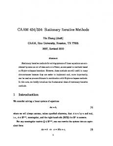
Figure 5: FT-GMRES on Diagonal problem, with different fault rates in inner solves’ SpMVs. Fault−Tolerant GMRES: Convergence vs. fault rate, with faulty SpMVs in the inner solves (deterministic faults)

0

2

4

6

8

10 12 14 Outer iteration number

16

18

20

22

Figure 7: FT-GMRES on mult dcop 03 problem, with different fault rates in inner solves’ SpMVs.

0

10

FT−GMRES(50,20) with error rate 0.000000 FT−GMRES(50,20) with error rate 0.100000 FT−GMRES(50,20) with error rate 0.300000 FT−GMRES(50,20) with error rate 0.500000

FT−GMRES(50,300): Fault rate vs. tolerance for mult_dcop_03 problem, with faulty SpMVs in the inner solves (deterministic faults) 300

Convergence tolerance 10−3 Convergence tolerance 10−6 Convergence tolerance 10−7.5

Number of outer iterations

250

−1

10

Convergence tolerance 10−9 200 150 100 50 0 0

0

2

4

6

8

10 12 14 Outer iteration number

16

18

20

22

Figure 6: FT-GMRES on Ill Stokes problem, with different fault rates in inner solves’ SpMVs. Nonrestarted GMRES’ residual norm often fails to be monotonic. Figures 5, 6, and 7 show only FT-GMRES (50 iterations per inner solve, 20 inner solves), with different fault rates for SpMV operations in the inner solves: no faults, 1 out of 10, 3 out of 10, and 5 out of 10 SpMVs faulty.5 We found that increasing the fault rate only decreases the FTGMRES convergence rate gradually. Finally, Figure 8 shows that, barring one outlier, the number of outer iterations to attain a given convergence rate increases little as the fault rate increases.

8.

CONCLUSIONS AND FUTURE WORK

The above section shows that FT-GMRES tolerates faults much better than standard GMRES. This holds even if we add robustness features to standard GMRES, and even if GMRES periodically restarts to throw away “bad” basis vectors. Our experiments also show that FT-GMRES’ convergence rate degrades gradually as the fault rate is increased, and that increasing the fault rate only modestly increases the total number of iterations (and therefore the total cost). While more experiments are needed, we think FT-GMRES and fault-tolerant iterative methods in general have great 5

In the 1 out of 10 case, only the tenth of every ten is faulty. The 3 out of 10 case uses the pattern 0, 0, 0, 0, 1, 0, 0, 1, 0, 1, and the 5 out of 10 case 1, 0, 1, 0, 1, 0, 0, 1, 0, 1.

0.05

0.1

0.15 0.2 Fault rate

0.25

0.3

0.35

0.4

Figure 8: Number of outer iterations to convergence for FT-GMRES (50 iterations per inner solve, max 300 outer iterations) on mult dcop 03 problem, vs. fault rate in the inner solves’ SpMVs, and the outer solves’ convergence tolerance. potential to improve solver robustness and relax hardware reliability constraints. The basic approaches we have used can be applied to many algorithms, greatly reducing the impact of the soft faults that are expected on future computing systems. Our work has also opened up interesting collaborations with systems researchers, to develop programming interfaces for varying reliability, reporting faults, and selective checkpointing. These collaborations have the potential to influence hardware-software codesign, especially at extreme scales, where energy requirements will force system designers to reduce hardware reliability and rely more on software approaches. Fault-tolerant algorithms thus have the potential to influence computer hardware in a way analogous to RISC (Reduced Instruction Set Computer) architectures [22], by encouraging beneficial trade-offs between hardware and software.

9.

ACKNOWLEDGMENTS

The authors thank the U.S. Department of Energy’s (DOE) Office of Advanced Scientific Computing and the DOE ASC program for funding this research.

10.

REFERENCES

[1] K. Asanovic, R. Bodik, B. C. Catanzaro, J. J. Gebis, P. Husbands, K. Keutzer, D. A. Patterson, W. L. Plishker, J. Shalf, S. W. Williams, and K. A. Yelick. The Landscape of Parallel Computing Research: A View from Berkeley. Technical Report UCB/EECS-2006-183, EECS Department, University of California, Berkeley, Dec 2006. See also the journal article Asanovic et al. [2]. [2] K. Asanovic, R. Bodik, J. W. Demmel, T. Keaveny, K. Keutzer, J. Kubiatowicz, N. Morgan, D. A. Patterson, K. Sen, J. Wawrzynek, D. Wessel, and K. A. Yelick. A View of the Parallel Computing Landscape. Communications of the ACM, 52(10):56–67, 2009. [3] J. Bahi, S. Contasset-Vivier, and R. Couturier. Parallel Iterative Algorithms: From Sequential to Grid Computing. Chapman and Hall / CRC, 2007. [4] L. S. Blackford, A. Cleary, J. Demmel, I. Dhillon, J. Dongarra, S. Hammarling, A. Petitet, H. Ren, K. Stanley, and R. C. Whaley. Practical experience in the dangers of heterogeneous computing. Technical Report UT-CS-96-330, University of Tennessee, Knoxville, July 1996. LAPACK Working Note #112. [5] G. Bronevetsky and B. de Supinski. Soft error vulnerability of iterative linear algebra methods. In Proceedings of the 22nd Annual International Conference on Supercomputing, ICS ’08, pages 155–164, New York, NY, USA, 2008. ACM. [6] A. Buttari, J. Dongarra, J. Kurzak, P. Luszczek, and S. Tomov. Computations to enhance the performance while achieving the 64-bit accuracy. Technical Report UT-CS-06-584, University of Tennessee Knoxville, November 2006. LAPACK Working Note #180. [7] M. Castro and B. Liskov. Practical Byzantine fault tolerance and proactive recovery. ACM Transactions on Computer Systems, 20(4):398–461, November 2002. [8] G. Chen, M. Kandemir, M. J. Irwin, and G. Memik. Compiler-directed selective data protection against soft errors. In In Proceedings of the Asia and South Pacific Design Automation Conference (ASPDAC), Shanghai, China, January 2005. [9] Z. Chishti, A. R. Alameldeen, C. Wilkerson, W. Wu, and S.-L. Lu. Improving cache lifetime reliability at ultra-low voltages. In Proceedings of the 42nd Annual IEEE/ACM International Symposium on Microarchitecture, MICRO 42, pages 89–99, New York, NY, USA, 2009. ACM. [10] T. A. Davis and Y. Hu. The University of Florida Sparse Matrix Collection. ACM Trans. Math. Softw. (to appear), 2011. [11] G. H. Golub and Q. Ye. Inexact preconditioned conjugate gradient method with inner-outer iteration. SIAM J. Sci. Comput., 21:1305–1320, 1999. [12] A. Greenbaum, V. Ptak, and Z. Strakos. Any nonincreasing convergence curve is possible for GMRES. SIAM J. Matrix Anal. Appl., 17:465–469, 1996. [13] I. S. Haque and V. S. Pande. Hard data on soft errors: A large-scale assessment of real-world error rates in GPGPU. In Proceedings of the 2010 10th IEEE/ACM International Conference on Cluster, Cloud and Grid

[14]

[15]

[16]

[17]

[18]

[19]

[20]

[21] [22]

[23] [24]

[25]

[26]

[27]

[28]

[29] [30]

Computing, CCGRID ’10, pages 691–696, Washington, DC, USA, 2010. IEEE Computer Society. V. E. Howle. Soft errors in linear solvers as integrated components of a simulation. In Presented at the Copper Mountain Conference on Iterative Methods, Copper Mountain, CO, April 9, 2010. K.-H. Huang and J. A. Abraham. Algorithm-based fault tolerance for matrix operations. IEEE Transactions on Computers, C-33(6), June 1984. T. Karnik, P. Hazucha, and J. Patel. Characterization of soft errors caused by single event upsets in CMOS processes. IEEE Trans. Dependable Secur. Comput., 1:128–143, April 2004. L. Lamport, R. Shostak, and M. Pease. The Byzantine Generals Problem. ACM Transactions on Programming Languages and Systems, 4(3):382–401, July 1982. P. T. Lin and J. N. Shadid. Towards large-scale multi-socket, multicore parallel simulations: Performance of an MPI-only semiconductor device simulator. J. Comput. Phys., 229:6804–6818, September 2010. K. Malkowski, P. Raghavan, and M. Kandemir. Analyzing the soft error resilience of linear solvers on multicore processors. In Proceedings of the Twenty-Fourth IEEE International Parallel and Distributed Processing Symposium (IPDPS), 2010. N. Miskov-Zivanov and D. Marculescu. Soft error rate analysis for sequential circuits. In Proceedings of the Conference on Design, Automation and Test in Europe, DATE ’07, pages 1436–1441, San Jose, CA, USA, 2007. EDA Consortium. B. Parhami. Defect, fault, error, . . . , or failure? IEEE Transactions on Reliability, 46(4), December 1997. D. A. Patterson and C. H. Sequin. RISC I: A Reduced Instruction Set VLSI Computer. In Proceedings of the Eighth Annual Symposium on Computer Architecture (ISCA). IEEE Computer Society Press, 1981. M. Rosenblum. The reincarnation of virtual machines. Queue, 2(5), 2004. Y. Saad. A flexible inner-outer preconditioned GMRES algorithm. SIAM J. Sci. Comput., 14:461–469, 1993. Y. Saad and M. H. Schultz. GMRES: A generalized minimal residual algorithm for solving nonsymmetric linear systems. SIAM J. Sci. Statist. Comput., 7:856–869, 1986. B. Schroeder, E. Pinheiro, and W.-D. Weber. DRAM errors in the wild: A large-scale field study. In SIGMETRICS / Performance 2009, June 15–19, 2009, Seattle, WA, USA, 2009. V. Simonici and D. B. Szyld. Flexible inner-outer Krylov subspace methods. SIAM J. Numer. Anal., 40(6):2219–2239, 2003. V. Simonici and D. B. Szyld. Theory of inexact Krylov subspace methods and applications to scientific computing. SIAM J. Sci. Comput., 25(2):454–477, 2003. J. E. Smith and R. Nair. The architecture of virtual machines. Computer, 38(5):32–38, May 2005. G. W. Stewart. Updating a rank-revealing U LV

[31]

[32]

[33]

[34]

decomposition. SIAM J. Matrix Anal. Appl., 14(2):494–499, April 1993. D. B. Szyld and J. A. Vogel. FQMR: A flexible quasi-minimal residual method with inexact preconditioning. SIAM J. Sci. Comput., 23(2):363–380, 2001. J. van den Eshof and G. L. G. Sleijpen. Inexact Krylov subspace methods for linear systems. SIAM J. Matrix Anal. Appl., 26(1):125–153, 2004. J. H. Wilkinson. Rounding Errors in Algebraic Processes. Prentice Hall, Englewood Cliffs, NJ, 1963. This work has been republished in an inexpensive Dover paperback edition. S. Yang, W. Wolf, W. Wang, N. Vijaykrishnan, and Y. Xie. Low-leakage robust SRAM cell design for sub-100nm technologies. In Proceedings of the 2005 Asia and South Pacific Design Automation Conference, ASP-DAC ’05, pages 539–544, New York, NY, USA, 2005. ACM.