Hindawi Publishing Corporation International Journal of Distributed Sensor Networks Volume 2015, Article ID 930585, 11 pages http://dx.doi.org/10.1155/2015/930585
Research Article Fault Tolerant Line-Based Barrier Coverage Formation in Mobile Wireless Sensor Networks Jie Shen,1 Zhibo Wang,2,3 and Zhi Wang1 1
Department of Control Science and Engineering, Zhejiang University, Hangzhou 310027, China School of Computer, Wuhan University, Wuhan 430072, China 3 Suzhou Institute of Wuhan University, Suzhou 215000, China 2
Correspondence should be addressed to Zhi Wang;
[email protected] Received 15 May 2015; Revised 23 August 2015; Accepted 2 September 2015 Academic Editor: Jianping He Copyright © 2015 Jie Shen et al. This is an open access article distributed under the Creative Commons Attribution License, which permits unrestricted use, distribution, and reproduction in any medium, provided the original work is properly cited. Barrier coverage is a fundamental problem for lots of applications in wireless sensor networks. In reality, sensor nodes’ true locations may not be known to us considering that not every sensor node is equipped with a GPS. The measured locations of sensor nodes obtained by applying node localization algorithm often have errors, which makes it difficult to form a line-based barrier with mobile sensor nodes. In this paper, we study how to efficiently schedule mobile sensor nodes to form a barrier when sensor nodes suffer from location errors. We explore the relationship between the existence of uncovered hole and location errors and find that the lengths of uncovered holes are decided by the cumulative location errors. We also propose a method in frequency domain to efficiently calculate the distributions of the cumulative location errors. The possibility of the existence of uncovered holes can be derived by analyzing the step responses of the cumulative location errors. Extensive experimental results demonstrate the effectiveness of the proposed algorithm.
1. Introduction Wireless sensor networks (WSNs) [1–6] have been widely used in a variety of application scenarios. In WSNs, the quality of sensing [7–10], which is often referred to as coverage, is a fundamental concern. Barrier coverage deploys sensor nodes in a long, narrow region of interest (ROI) which carries out detecting the targets when they penetrate into the region. It finds significant application in WSNs. For example, in the application of border surveillance, we are able to detect unauthorized intrusions by deploying sensor nodes along the boundary of interest. The first and most important aspect to form a barrier is how to design sensor nodes deployment. When the sensor nodes are placed to the expected locations, the quality of barrier coverage is guaranteed. However, in actual applications, most cases of the ROI are in harsh environment, which make it difficult to obtain the expected locations and deploy the nodes there. Sensor nodes are deployed randomly in most practical cases; for example, they can be dropped from aircraft [11]. To this end, the sensor nodes are not deployed
to the expected locations initially, and they could not form a barrier. Fortunately, thanks to recent advances in mobilityassistant technology, sensor nodes have the ability to move around to carry out tasks [12, 13]. Hence, a barrier coverage could be formed by controlling the senor mobility. Firstly, each mobile sensor node obtains its location before moving to the expected locations. Therefore, the problem of achieving barrier coverage is covert to the localization problem of mobile nodes. Equipping GPS receivers on each node to get the accurate location information is too costexpensive. Hence, in practical use, only several nodes are equipped with GPS receivers. The other nodes are located by integrating the relative locations to their neighboring nodes using localization algorithms. In the past years, lots of localization algorithms have been proposed, such as Time of Arrival (TOA) [14], Time Difference of Arrival (TDOA) [15, 16], Angle of Arrival (AOA) [17, 18], and Received Signal Strength Indicator (RSSI) [19–21]. However, the location results provided by these algorithms have low accuracy and in most cases with location errors. Due to location errors, mobile nodes’ measured locations are different from their
2
International Journal of Distributed Sensor Networks
actual locations. Thus, they cannot stop and be deployed at the expected locations in real applications. To guarantee the quality of barrier coverage, barrier formation should be adaptive to the location errors. However, little literature considers the effects of location errors. Moreover, the location errors of the localization algorithms are diverse and may follow a random distribution. Traditional methods always analyze the worst cases, that is, the lower and upper bounds. However, worst case analysis is always conservative and hard to capture the higherorder location error characteristics. For example, node A is equipped with a GPS receiver; node B is located relative to node A, and the location error follows a uniform distribution: 𝑈[−3 m, 3 m]; node C is located relative to node B, and the location error follows 𝑈[−5 m, 5 m]. Thus, the measured location of node C deviates from its actual location, and the deviation equals the cumulative location error. The cumulative location error follows the joint distribution of 𝑈[−3 m, 3 m] and 𝑈[−5 m, 5 m]. From the error distribution, we could get the probability of location error of any value other than the lower and upper bounds (−8 m and 8 m). However, previous work rarely studied the distributions of the cumulative location errors. In this paper, we investigate how to efficiently schedule mobile sensor nodes to form a barrier when sensor nodes suffer from undetermined location errors. Firstly, we investigate how the uncovered holes are generated by the location errors and find that the lengths of uncovered holes are decided by the cumulative location errors. Then we analyze how to calculate the distributions of cumulative location errors. Since each location error follows a distribution, convoluting the distributions of individual location errors to get the distribution of the cumulative location error is inefficient. Its computational cost is extremely high when the network is large. In this paper, we calculate the location errors in the frequency domain. Convolution is converted to multiplication and the computation complexity is heavily reduced. Third, after the cumulative location errors are obtained in frequency domain, we analyze the characteristics of their step responses (e.g., probability distribution functions). Then, the probability of uncovered holes existing could be easily obtained from the step responses. Finally, when the possibilities are high, we reduce the possibilities by deploying more nodes, equipping more GPSs, or improving sensing range to guarantee the quality of barrier coverage adaptively. To the best of our knowledge, our work is the first applying frequency analysis on studying barrier coverage problem when nodes have location errors. The major intellectual contributions of this paper are summarized as follows: (i) We theoretically analyze the relationships between the lengths of the uncovered holes and the location errors. The mathematical expressions of calculating the uncovered holes’ length from the cumulative location errors are given. (ii) When each location error follows a distribution, we give an efficient method to calculate the distribution of the cumulative location error in frequency domain.
(iii) We propose a method of analyzing the step response of the cumulative location error to get the probability of the uncovered hole existing. (iv) We study some cases to show how to use our framework and guarantee the quality of barrier coverage adaptively. The rest of this paper is organized as follows. Section 2 surveys the related work and Section 3 analyzes the barrier coverage when location errors exist. We give theoretical expressions of calculating the uncovered hole length in Section 4. Then in Section 5 we calculate the cumulative location errors in frequency domain and get the probabilities of the uncovered holes existing. Section 6 gives examples of using our framework and corresponding evaluation and Section 7 provides conclusions.
2. Related Work Barrier coverage is a fundamental problem for lots of applications in wireless sensor networks and has been widely researched. Kumar et al. [22] firstly defined the notion of kbarrier coverage and introduced weak and strong coverage in a belt region. Liu et al. [23] proposed a solution for strong barrier coverage when sensor nodes are randomly deployed according to a Poisson point distribution process. Li et al. [24] investigated the weak k-barrier coverage problem and derive a lower bound for the probability of weak kbarrier coverage. Since most cases of the ROI are in harsh environment and difficult for human being to reach, Saipulla et al. [11] investigated barrier coverage with airdropped wireless sensors under line-based deployments and give a lower bound for the existence of barrier coverage. In [25], He et al. showed the suboptimality of line-based deployment when the length of shortest line segment is larger than that of shortest path and for the first time quantified the need of curve-based deployment; then they introduced a concept of distance-continuous curve and provided an algorithm to obtain the optimal sensor deployment when the deployment curve is distance continuous. Chen et al. [26, 27] proposed the methods of scheduling sensors energy efficiently while guaranteeing the detection probability of any intrusion across the region based on probabilistic sensing model, which is a more actual sensing model. Due to recent technological advances, nodes have the ability to move around to carry out tasks. Barrier coverage in mobile sensor network is a hot research area. He et al. [28] guaranteed that each point along the barrier line is monitored periodically by mobile sensors by using a periodic monitoring scheduling algorithm. Saipulla et al. [29] presented a method which could construct the maximum number of barriers under the constraints of sensor mobility. Shen et al. [30] found that barrier coverage could be achieved with fewer mobile sensors than stationary sensors when applying random deployment. Wang et al. [31] proposed a method of using minimum number of mobile sensor nodes to improve barrier coverage when the stationary nodes are not forming a barrier after initial deployment. He et al. [32] designed a periodic monitoring scheduling algorithm in which each point along
International Journal of Distributed Sensor Networks
3 if we denote 𝐷 = 𝐿/𝑁, the node to the left end is deployed at location 𝐷/2, the node to the right end is deployed at location 𝑁𝐷/2, and the interval between any two neighboring nodes is 𝐷. To guarantee the overlap of any two neighboring nodes, condition 𝐷 ≤ 2𝑟𝑠 must be satisfied. Considering the limitation of the sensing range and communication range of the nodes, the minimum number of nodes we need to form a barrier to cover 𝐿 is
Intruder A rs
rc Intruder B
Figure 1: Sensing range and communication range of sensor node.
the barrier line is monitored periodically by mobile sensors and propose a coordinated sensor patrolling algorithm to further improve the barrier coverage, where each sensor’s current movement strategy is derived from the information of intruder arrivals in the past. Using mobility-assistant nodes in randomly deployment barrier coverage can achieve higher quality sensing performance if they could move to the designed locations. However, due to high equipment cost, not all mobile nodes are equipped with GPS receivers. We locate them using typical localization algorithms. However, location errors exist which will significantly affect the quality of coverage. Thus, in this paper, we investigate how to efficiently schedule mobile sensor nodes to form a barrier when sensor nodes obtain locations with errors.
3. Barrier Coverage When Location Errors Exist Mobile wireless sensor networks usually consist of large number of mobile sensor nodes. We denote 𝑆𝑖 as the index of 𝑖th sensor node. Each sensor node can detect the target or event if it is within the sensing range and then the sensor nodes can communicate with each other. We assume that all sensor nodes have the same sensing range and communication range. As shown in Figure 1, the sensing range is denoted as 𝑟𝑠 . A sensor node can detect an intruder within its sensing range, for example, intruder A, in Figure 1. However, it cannot detect the intruder beyond its sensing range 𝑟𝑠 , such as intruder B. The communication range is denoted as 𝑟𝑐 , which is larger than the sensing range 𝑟𝑠 . We assume that 𝑟𝑐 > 2𝑟𝑠 . We construct the model of the region of interest (ROI) with a closed line interval [0 : 𝐿], whose line has two endpoints, 0 and 𝐿 > 0. The sensor nodes are deployed on this line to form a barrier coverage. The total number of nodes is 𝑁, and these 𝑁 nodes are uniformly deployed, which means,
𝑁min = ceil (
𝐿 ). 2𝑟𝑠
(1)
As shown in Figure 2(a), we deploy 𝑁min nodes on line 𝐿. 𝐷 is set to 2𝑟𝑠 , and node 𝑆𝑖 is deployed at (2𝑖 − 1)𝑟𝑠 . If the nodes are deployed at these locations, the whole line 𝐿 could be successfully covered. However, in practical scenario, the ROI is probably in a harsh environment, and sensor nodes are usually deployed randomly. In such case, the sensor nodes are not deployed in the expected location initially, and the barrier cannot be formed. Fortunately, with mobility-assistant technology, the mobile nodes can move to the designed locations to form a barrier. However, it is too expensive to equip each node with a GPS receiver. In a typical network, only several nodes are equipped with a GPS receiver, which act as the beacon nodes. Then, we can use localization algorithms to locate other nodes that are neighboring these beacon nodes. When these locations are obtained, they also become beacon nodes to the other neighboring nodes. With such method, all the nodes’ locations can be obtained. Actually, there is localization error in practical process. Take example of node 𝑆𝑎 , with its true location being 𝑥𝑎 , and the corresponding measured location is denoted by 𝑥̂𝑎 . If 𝑆𝑎 is equipped with a GPS receiver, then 𝑥̂𝑎 = 𝑥𝑎 . If there is a node 𝑆𝑏 neighboring node 𝑆𝑎 which needs to be located, using the above-mentioned localization algorithms, we can get the ̂ 𝑎,𝑏 between 𝑆𝑎 and measured location of 𝑆𝑏 and the distance 𝐿 𝑆𝑏 . When 𝑆𝑏 is on the left of 𝑆𝑎 , the measured location of 𝑆𝑏 is ̂ 𝑎,𝑏 ; 𝑥̂𝑏 = 𝑥̂𝑎 − 𝐿
(2)
otherwise, the measured location of 𝑆𝑏 is ̂ 𝑎,𝑏 . 𝑥̂𝑏 = 𝑥̂𝑎 + 𝐿
(3)
In wireless sensor networks, none of the existing localization algorithms can obtain perfectly accurate location; that is, the location errors exist actually. Hence, we get ̂ 𝑎,𝑏 − 𝐿 𝑎,𝑏 , Δ𝐿𝑏hop = 𝐿
(4)
̂ 𝑎,𝑏 denotes the measured distance between node 𝑆𝑎 where 𝐿 and node 𝑆𝑏 and 𝐿 𝑎,𝑏 denotes the actual distance between these two nodes; Δ𝐿𝑏hop denotes the one-hop location error of node 𝑆𝑏 . Definition 1. The one-hop location error 𝐿 hop is the measurement error of the distance from sensor node to its corresponding beacon node.
4
International Journal of Distributed Sensor Networks D 0
···
x1
x2
xN−1
xN
S1
S2
SN−1
SN
L
x
0
···
x1
x2
xN−1
xN
S1
S2
SN−1
SN
Uncovered hole
x
L
Uncovered hole
(a)
(b)
Figure 2: An example of line-based barrier coverage: (a) nodes are deployed in the expected location; minimum number of nodes is used to form a barrier; (b) when location error exists, the barrier has uncovered holes on it.
While there is location error, mobile nodes cannot move to the optimized locations. We take an example to demonstrate the impact of the location errors. As shown in Figure 2(b), we utilize 𝑁min number of mobile nodes to cover the line 𝐿, with several nodes being equipped with a GPS receiver. However, most of the nodes need to be located by using localization algorithms. For 𝑖th node which does not have any GPS receiver, its measured location is 𝑥̂𝑖 . When the sensor node finishes moving, we get 𝑥̂𝑖 = (2𝑖 − 1) 𝑟𝑠 .
(5)
Sp
Sp
Sq
Sq Uncovered hole
(a)
(b)
Figure 3: Node 𝑆𝑝 is the beacon of node 𝑆𝑞 : (a) nodes overlap with each other and no uncovered hole exists; (b) nodes do not overlap with each other and an uncovered hole exists.
However, due to location error, we get 𝑥𝑖 ≠ 𝑥̂𝑖 = (2𝑖 − 1) 𝑟𝑠 ;
(6)
that is, its actual location 𝑥𝑖 does not equal the expected location. Thus, as shown in Figure 2(b), such condition incurs uncovered holes on the barrier.
4. Models of the Uncovered Holes
4.1. The First Type of the Uncovered Hole. The first type of uncovered hole is shown as in Figure 3. There are two neighboring nodes, nodes 𝑆𝑝 and 𝑆𝑞 , in the network. Node 𝑆𝑝 is the beacon node of 𝑆𝑞 . Due to the location error, an uncovered hole may exist between the locations of them. We get the following. Theorem 2. For two neighboring nodes, nodes 𝑆𝑝 and 𝑆𝑞 in the network, when node 𝑆𝑝 is the beacon node of node 𝑆𝑞 , the length of the uncovered hole between them is 𝑞
̂ 𝑥̂𝑞 − 𝑥̂𝑝 = 𝐷 = 𝐿 𝑝,𝑞 .
(8)
Combining with (4) and (8), we get
In the above section, we show that due to the existence of the location errors the nodes cannot move to the expected locations. Hence, this situation incurs uncovered holes on the barrier. The uncovered holes could be classified into three categories: (1) the uncovered hole between two neighboring nodes where one node is located based on the other node; (2) the uncovered hole between two neighboring nodes where the two nodes are not located based on one another; (3) the uncovered holes between the leftmost (or rightmost) node and the left (or right) endpoints of 𝐿. We define them as the first, second, and third type of uncovered hole, respectively, in the following description. We will give detailed analysis of these three types of uncovered holes in this section.
ℎ𝑡𝑝1 = max (0, 𝐷 − 2𝑟𝑠 − Δ𝐿 ℎ𝑜𝑝 ) .
Proof. The interval between nodes 𝑆𝑝 and 𝑆𝑞 is set to 𝐷; we get
(7)
𝑞
𝑞
̂ 𝐿 𝑝,𝑞 = 𝐿 𝑝,𝑞 − Δ𝐿 hop = 𝐷 − Δ𝐿 hop .
(9)
As shown in Figure 3(a), when 2𝑟𝑠 − 𝐿 𝑝,𝑞 > 0, nodes 𝑆𝑝 and 𝑆𝑞 overlap with each other. Thus, there is no uncovered hole between these two locations; that is, ℎ𝑝,𝑞 = 0. However, as shown in Figure 3(b), when 2𝑟𝑠 − 𝐿 𝑝,𝑞 < 0, nodes 𝑆𝑝 and 𝑆𝑞 do not overlap with each other. There is an uncovered hole between them, and its corresponding length is ℎ𝑝,𝑞 = 𝐿 𝑝,𝑞 − 2𝑟𝑠 .
(10) 𝑞
Combining with (9) and (10), we get ℎ𝑝,𝑞 = 𝐷 − 2𝑟𝑠 − Δ𝐿 hop .
4.2. The Second Type of the Uncovered Hole. The second type of uncovered hole is shown as in Figure 4. There are two neighboring nodes, nodes 𝑆𝑑 and 𝑆𝑒 , in the network. Node 𝑆𝑑−𝑖 ’s beacon node is node 𝑆𝑑−𝑖−1 , and node 𝑆𝑑−𝑀 is equipped with a GPS receiver. Similarly, node 𝑆𝑒+𝑖 ’s beacon node is 𝑆𝑒+𝑖+1 , and node 𝑆𝑒+𝐾 is equipped with a GPS receiver. 𝑀 is defined as the hops from node 𝑆𝑑 to its nearest GPS node. 𝐾 is defined as the hops from node 𝑆𝑒 to its nearest GPS node. When 𝑀 = 0 or 𝐾 = 0, there is a GPS receiver equipped on 𝑆𝑑 or 𝑆𝑒 , respectively. We get the following.
International Journal of Distributed Sensor Networks ···
···
···
Sd−M
Sd−1
Sd
Se
Se+1
5 ···
···
···
···
Sd−M
Se+K
Sd−1
Sd
Se
Se+1
···
Se+K
Uncovered hole
Node without any GPS receiver Node with a GPS receiver
Node without any GPS receiver Node with a GPS receiver
(a)
(b)
Figure 4: 𝑆𝑑 and 𝑆𝑒 are not located based on the other: (a) no uncovered hole exists; (b) an uncovered hole exists.
···
···
0 Sl
Sl+1
Sr−Q
Sl+P
···
···
Sr−1
Sr L
x
0
Sl
Sl+1
···
···
Sr−Q
Sl+P
Sr−1
Uncovered hole
Node without any GPS receiver Node with a GPS receiver
Sr
L x
Uncovered hole
Node without any GPS receiver Node with a GPS receiver
(a)
(b)
Figure 5: The uncovered hole between the leftmost (rightmost) node and the left (right) endpoint of 𝐿: (a) uncovered holes do not exist; (b) uncovered holes exist.
Theorem 3. For two neighboring nodes, nodes 𝑆𝑑 and 𝑆𝑒 in the network, where the two nodes are not located based on one another, 𝐾−1
ℎ𝑡𝑝2 = max (0, 𝐷 − 2𝑟𝑠 + ∑ Δ𝐿𝑑+𝑖 ℎ𝑜𝑝 ) .
(11)
𝑖=1−𝑀
Proof. Since the interval between nodes 𝑆𝑑 and 𝑆𝑒 is set to 𝐷, we get 𝑥̂𝑒 − 𝑥̂𝑑 = 𝐷.
(12)
̂ 𝑑−𝑀,𝑑−𝑀+1 + ⋅ ⋅ ⋅ + 𝐿 ̂ 𝑑−1,𝑑 . 𝑥̂𝑑 = 𝑥̂𝑑−𝑀 + 𝐿
(13)
Obviously, we get
Combining with (4), we get 𝑥̂𝑑 = 𝑥̂𝑑−𝑀 + (𝐿 𝑑−𝑀,𝑑−𝑀+1 + ⋅ ⋅ ⋅ + 𝐿 𝑑−1,𝑑 ) 𝑀
(14)
+ ∑Δ𝐿𝑑−𝑖+1 hop . 𝑖=1
Since 𝑆𝑑−𝑀 is equipped with GPS receiver, we have 𝑥̂𝑑−𝑀 = 𝑥𝑑−𝑀. Hence, we get 𝑥̂𝑑 = 𝑥𝑑−𝑀 + (𝐿 𝑑−𝑀,𝑑−𝑀+1 + ⋅ ⋅ ⋅ + 𝐿 𝑑−1,𝑑 ) 𝑀
𝑀
𝑖=1
𝑖=1
𝑑−𝑖+1 + ∑Δ𝐿𝑑−𝑖+1 hop = 𝑥𝑑 + ∑Δ𝐿 hop .
(15)
𝐾
𝑒+𝑗−1
𝑗=1
ℎ𝑑,𝑒 = 𝑥𝑒 − 𝑥𝑑 − 2𝑟𝑠 .
(17)
Combining with (12), (15), (16), and (17), we get ℎ𝑑,𝑒 = 𝐷 − 𝑒+𝑗−1 𝐾 𝑑−𝑖+1 2𝑟𝑠 + ∑𝑀 𝑖=1 Δ𝐿 hop + ∑𝑗=1 Δ𝐿 hop . Since nodes 𝑆𝑑 and 𝑆𝑒 are neighboring nodes, we get 𝑒 = 𝑑 + 1. Hence, ℎ𝑑,𝑒 = 𝐷 − 2𝑟𝑠 + 𝑑+𝑖 ∑𝐾−1 𝑖=1−𝑀 Δ𝐿 hop . 4.3. The Third Type of the Uncovered Hole. The third type of uncovered hole is shown as in Figure 5. Node 𝑆𝑙 is the leftmost node of the network, and node 𝑆𝑟 is the rightmost node of the network. Node 𝑆𝑙+𝑖 ’s beacon node is 𝑆𝑙+𝑖−1 , and 𝑆𝑙+𝑃 is equipped with a GPS receiver. Similarly, node 𝑆𝑟−𝑗 ’s beacon node is 𝑆𝑟−𝑗−1 , and 𝑆𝑟−𝑄 is equipped with a GPS receiver. 𝑃 is defined as the hops from node 𝑆𝑙 to its nearest GPS node. 𝑄 is defined as the hops from node 𝑆𝑟 to its nearest GPS node. When 𝑃 = 0 or 𝑄 = 0, GPS receivers are equipped on 𝑆𝑙 or 𝑆𝑟 , respectively. Theorem 4. The length of the uncovered hole between the leftmost node 𝑆𝑙 and the left endpoint of 𝐿 is
Similarly, for 𝑆𝑒 , we get 𝑥̂𝑒 = 𝑥𝑒 − ∑Δ𝐿 hop .
As shown in Figure 4(a), when 𝑥𝑒 − 𝑥𝑑 − 2𝑟𝑠 < 0, that is, nodes 𝑆𝑑 and 𝑆𝑒 overlap with each other, there is no uncovered hole between these two locations. However, as shown in Figure 4(b), when 𝑥𝑒 − 𝑥𝑑 − 2𝑟𝑠 > 0, that is, they have no overlapping area, there is an uncovered hole between them and its length is
(16)
ℎ𝑡𝑝3𝑙 = max (0,
𝑃 𝐷 − 𝑟𝑠 + ∑Δ𝐿𝑙+𝑖−1 ℎ𝑜𝑝 ) . 2 𝑖=1
(18)
6
International Journal of Distributed Sensor Networks
And the length of the uncovered hole between the rightmost node 𝑆𝑟 and the right endpoint of 𝐿 is ℎ𝑡𝑝3𝑟
𝑄
𝐷 𝑟−𝑗+1 = max (0, − 𝑟𝑠 + ∑Δ𝐿 ℎ𝑜𝑝 ) . 2 𝑗=1
(19)
Proof. For the uncovered hole between the leftmost node and the left endpoint of 𝐿, since the leftmost node is set to be deployed at 𝐷/2, we get 𝑥̂𝑙 =
𝐷 . 2
(20)
Then, we get ̂ 𝑙+𝑃−1,𝑙+𝑃 − ⋅ ⋅ ⋅ − 𝐿 ̂ 𝑙,𝑙+1 . 𝑥̂𝑙 = 𝑥̂𝑙+𝑃 − 𝐿
(21)
Since node 𝑆𝑙+𝑃 is equipped with a GPS receiver, we can get 𝑥̂𝑙+𝑃 = 𝑥𝑙+𝑃 . Combining with (4) and (21), we get 𝑃
𝑥̂𝑙 = 𝑥𝑙+𝑃 − (𝐿 𝑙+𝑃−1,𝑙+𝑃 + ⋅ ⋅ ⋅ + 𝐿 𝑙+1,𝑙 ) − ∑Δ𝐿𝑙+𝑖−1 hop 𝑖=1
𝑃
(22)
5. Analysis of Coverage in Frequency Domain We have introduced the uncovered holes in aforementioned section and find that the uncovered holes are determined by the node location errors. For practical consideration, the location errors are usually not fixed. Each one-hop location error follows a random distribution which can be obtained by theoretical analysis or from numerous experiments. The cumulative location error follows a superimposed distribution, and the probability density function equals the convolution of the probability density functions of the individual one-hop location errors. Let Δ𝐿 hop denote the one-hop location error in the network. The probability density function of Δ𝐿 hop is denoted 𝑞 by 𝑓hop (𝑡). Considering Theorems 2, 3, and 4, Δ𝐿 hop represent 𝑑+𝑖 the (cumulative) location error part in (7), ∑𝐾−1 𝑖=1−𝑀 Δ𝐿 hop in 𝑟−𝑗+1
𝑄 (11), ∑𝑃𝑖=1 Δ𝐿𝑙+𝑖−1 hop in (18), and ∑𝑗=1 Δ𝐿 hop in (19), respectively. For the cumulative location errors, we get the following. 𝑞 We define Δ𝐿 𝑡𝑝1 = Δ𝐿 hop , and its probability density function is denoted by 𝑓𝑡𝑝1 (𝑡). We get 𝑞
= 𝑥𝑙 − ∑Δ𝐿𝑙+𝑖−1 hop .
𝑓𝑡𝑝1 (𝑡) = 𝑓hop (𝑡) .
𝑖=1
As shown in Figure 5(a), when 𝑥𝑙 < 𝑟𝑠 , there is no uncovered hole. However, as shown in Figure 5(b), when 𝑥𝑙 > 𝑟𝑠 , we have ℎ𝑙 = 𝑥𝑙 − 𝑟𝑠 .
(23)
Combing with (20), (22), and (23), the length of the uncovered hole between the leftmost node and the left endpoint of 𝐿 is ℎ𝑙 = 𝐷/2 − 𝑟𝑠 + ∑𝑃𝑖=1 Δ𝐿𝑙+𝑖−1 hop . Similarly, we can prove ℎ𝑟 = max(0, 𝐷/2 − 𝑟𝑠 + 𝑟−𝑗+1 ∑𝑄 𝑗=1 Δ𝐿 hop ). We have introduced the three types of uncovered holes. From Theorems 2, 3, and 4, we find the following: (i) The uncovered holes are decided by the neighboring nodes’ interval 𝐷, the sensing range 𝑟𝑠 , and the location errors. When we have smaller 𝐷 or larger 𝑟𝑠 , the uncovered hole is smaller. However, a smaller 𝐷 value means deploying more sensor nodes, and a larger 𝑟𝑠 value means using more expensive sensor. Both of them finally increase the cost of the system. (ii) The first type of uncovered hole is decided by the onehop location error. (iii) The second and third types of uncovered holes are decided by the cumulative location errors. Thus, as the network scale gets larger, they can be much more complicated to analyze than the first type of uncovered hole. (iv) In an actual network, the three types of uncovered holes are not separated. For example, when Δ𝐿 hop is negative and smaller, the first type of uncovered hole will disappear; however, the second and third type of uncovered holes may become larger. This situation incurs complicated analysis of the uncovered holes.
(24)
𝑑+𝑖 Let Δ𝐿 𝑡𝑝2 = ∑𝐾−1 𝑖=1−𝑀 Δ𝐿 hop , and its probability density function is denoted by 𝑓𝑡𝑝2 (𝑡). We have 𝑑−𝑀+1 𝑑−𝑀+2 𝑑+𝐾−1 𝑓𝑡𝑝2 (𝑡) = 𝑓hop (𝑡) ⊗ 𝑓hop (𝑡) ⋅ ⋅ ⋅ ⊗ 𝑓hop (𝑡) .
(25)
Let Δ𝐿 𝑡𝑝3𝑙 = ∑𝑃𝑖=1 Δ𝐿𝑙+𝑖−1 hop , and its probability density function 𝑟−𝑗+1
is denoted by 𝑓𝑡𝑝3𝑙 (𝑡). Let Δ𝐿 𝑡𝑝3𝑟 = ∑𝑄 𝑗=1 Δ𝐿 hop , and its probability density function is denoted by 𝑓𝑡𝑝3𝑟 (𝑡). We have 𝑙 𝑙+1 𝑙+𝑃 𝑓𝑡𝑝3𝑙 (𝑡) = 𝑓hop (𝑡) ⊗ 𝑓hop (𝑡) ⋅ ⋅ ⋅ ⊗ 𝑓hop (𝑡) , 𝑟 𝑟−1 𝑟−𝑄 𝑓𝑡𝑝3𝑟 (𝑡) = 𝑓hop (𝑡) ⊗ 𝑓hop (𝑡) ⋅ ⋅ ⋅ ⊗ 𝑓hop (𝑡) .
(26)
Thus, we need to convolute the one-hop location error distributions to get the distributions of the cumulative location errors. When the distributions of the cumulative location errors, that is, 𝑓𝑡𝑝1 (𝑡), 𝑓𝑡𝑝2 (𝑡), 𝑓𝑡𝑝3𝑙 (𝑡), and 𝑓𝑡𝑝3𝑟 (𝑡), are obtained, we can analyze the uncovered holes. However, the computation of convolutions in (25) and (26) is extremely high when the network scale is large. Thus, to obtain the lengths of the uncovered holes and guarantee coverage, the key problem is how to calculate the distributions of the cumulative location errors effectively. To solve this problem, we propose an efficient method in frequency domain. Let 𝑓(𝑡) denote the probability density function of the location error which is in time domain. It could be converted into frequency domain by Laplace Transform as follows: ∞
F (𝑠) = L [𝑓 (𝑡)] = ∫ 𝑒−𝑠𝑡 𝑓 (𝑡) 𝑑𝑡, 0
(27)
where L is the operator of Laplace Transform. After the probability density function of the location error is converted to the frequency domain, convolution is converted to multiplication. Thus, the computation complexity becomes much
International Journal of Distributed Sensor Networks
7
lower. Meanwhile, if we obtained F(𝑠) in frequency domain, it could easily get 𝑓(𝑡) by using Inverse Laplace Transform as follows: 𝑓 (𝑡) = L−1 [F (𝑠)] =
1 𝜎+𝑗∞ 𝑠𝑡 𝑒 F (𝑠) 𝑑𝑠. ∫ 𝑗2𝜋 𝜎−𝑗∞
(28)
By using Laplace Transform and converting distributions to the frequency domain, we calculate the cumulative location errors for different types of uncovered holes as 𝑞
F𝑡𝑝1 (𝑠) = L [𝑓𝑡𝑝1 (𝑡)] = Fhop (𝑠) ; F𝑡𝑝2 (𝑠) = L [𝑓𝑡𝑝2 (𝑡)] =
𝐾−1
∏ F𝑑+𝑖 hop 𝑖=1−𝑀
(29) (𝑠) ;
(30)
𝑃
F𝑡𝑝3𝑙 (𝑠) = L [𝑓𝑡𝑝3𝑙 (𝑡)] = ∏F𝑙+𝑖−1 hop (𝑠) ;
(31)
𝑖=1 𝑄
𝑟−𝑗+1
F𝑡𝑝3𝑟 (𝑠) = L [𝑓𝑡𝑝3𝑟 (𝑡)] = ∏Fhop (𝑠) .
(32)
Let F(𝑠) denote the cumulative location error in frequency domain. We give unit step function as 𝑢(𝑡) = 1, if 𝑡 ≥ 0; 0, if 𝑡 < 0. Step response means the response (output) to a unit step-function input. In control theory, the step response of F(𝑠) equals the probability distribution function of the cumulative location error in time domain. We give the explanations here. Let 𝑦𝑢(𝑡) denote the time response for 𝑢(𝑡). We can get 1 ⋅ F (𝑠) . 𝑠
(33)
The step response can be obtained by Inverse Laplace Transform as 𝑡 1 𝑦𝑢(𝑡) = L−1 [ ⋅ F (𝑠)] = ∫ 𝑓 (𝜏) 𝑑𝜏 = 𝐹 (𝑡) , 𝑠 0
(34)
where 𝐹(𝑡) is the probability distribution function of the cumulative location error in time domain. Based on the step responses, it is feasible to analyze the uncovered holes. For the first type of uncovered hole, its length is ℎ𝑡𝑝1 = 𝑞 max(0, 𝐷 − 2𝑟𝑠 − Δ𝐿 hop ) = max(0, 𝐷 − 2𝑟𝑠 − Δ𝐿 𝑡𝑝1 ). Thus, when there is no uncovered hole, it satisfies Δ𝐿 𝑡𝑝1 ≥ 𝐷 − 2𝑟𝑠 . The probability distribution function (i.e., step response) of Δ𝐿 𝑡𝑝1 is 𝐹𝑡𝑝1 (𝑡). We have 𝑝𝑡𝑝1 = 1 − 𝐹𝑡𝑝1 (𝑡 ≥ 𝐷 − 2𝑟𝑠 ) ,
(35)
which means the probability of the first type of uncovered hole is 𝑝𝑡𝑝1 . Similarly, the probability of the second type of uncovered hole existing is 𝑝𝑡𝑝2 = 1 − 𝐹𝑡𝑝2 (𝑡 ≤ 2𝑟𝑠 − 𝐷) .
The length of the region of interest 𝐿 (m) The sensing range 𝑟𝑠 (m) The number of nodes deployed originally 𝑁 The number of nodes added 𝑁∗ The number of GPS receivers equipped originally The number of GPS receivers added
(36)
2000 50, 60, and 70 21 5, 10, and 15 1 1, 2, and 3
The probability of the third type of uncovered hole existing at the left endpoint of 𝐿 is 𝑝𝑡𝑝3𝑙 = 1 − 𝐹𝑡𝑝3𝑙 (𝑡 ≤ 𝑟𝑠 −
𝐷 ), 2
(37)
and the probability of the third type of uncovered hole existing at the right endpoint of 𝐿 is 𝑝𝑡𝑝3𝑟 = 1 − 𝐹𝑡𝑝3𝑟 (𝑡 ≤ 𝑟𝑠 −
𝑖=1
L [𝑦𝑢(𝑡) ] = L [𝑢 (𝑡)] ⋅ F (𝑠) =
Table 1: System constants and simulation parameters.
𝐷 ). 2
(38)
We have developed the theoretical framework to model and analyze the uncovered holes. The procedures are shown in Algorithm 5. Algorithm 5. The theoretical framework to model and analyze the uncovered holes is as follows: (1) Obtain individual one-hop location error distributions of the network and convert them into frequency domain using Laplace Transform. (2) Calculate the distributions of the cumulative location errors in frequency domain by multiplications. (3) Analyze the step responses to get the probability of having uncovered holes on the barrier.
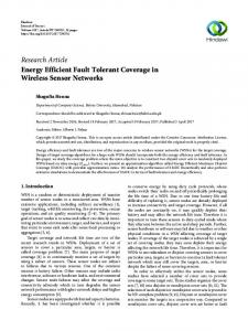
6. Evaluation In previous sections, we have introduced our framework of analyzing the uncovered holes. In this section, we give some examples to show how to use the framework. The parameters of the simulations are summarized in Table 1. The length of the region of interest 𝐿 is 2000 m and the sensing range 𝑟𝑠 is 50 m. We deploy 21 mobile nodes to form a barrier. The designed interval between any two neighboring nodes is 𝐷 = 𝐿/𝑁 = 2000/21 = 95 m. Obviously, when each node is equipped with a GPS receiver, that is, every node can obtain its accurate location, we can form a perfect barrier. However, as shown in Figure 6(a), due to high cost, only node 𝑆1 is equipped with a GPS receiver. The locations of other nodes are obtained by using localization algorithms. Node 𝑆𝑖 is 𝑆𝑖+1 ’s beacon node. The results provided by the location algorithms contain location errors. The probability 𝑖 (𝑡) of any one-hop location error is density function 𝑓hop −2𝑡
{2𝑒 𝑖 𝑓hop (𝑡) = { 0, {
,
𝑡 ≥ 0, 𝑡 < 0,
which follows an exponential distribution.
(39)
8
International Journal of Distributed Sensor Networks ···
0
S1
S2
S3
S4
S18
S19 S20
L
S21
x
···
0
S1
Uncovered hole
S2
S3
S4
S22 S23 S24
S25 S26 L
x
Node without any GPS receiver Node with a GPS receiver
Node without any GPS receiver Node with a GPS receiver
(b)
(a)
0
···
S1
S2
S3
S4
S5
S6
S7
S21
L
x
Uncovered hole
Uncovered hole Node without any GPS receiver Node with a GPS receiver
(c)
1
1
0.9
0.9
0.8
0.8
0.7
0.7 Probability
Probability
Figure 6: The example systems: (a) we deploy 21 nodes, and only node 𝑆1 is equipped with a GPS receiver; (b) we add some nodes into the network; (c) more nodes are equipped with a GPS receiver.
0.6 0.5 0.4
0.5 0.4 0.3
0.2
0.2
0.1
0.1 0 0
0.5
1
1.5 2 2.5 3 3.5 One-hop location error (m)
4
4.5
5
(12.5, 0.87)
0.6
0.3
0
(22.5, 1)
(0, 2.5) 0
5
10 15 20 Cumulative location error (m) rs = 70
rs = 50 rs = 60
(a)
25
(b)
Figure 7: The step responses: (a) step response of F𝑡𝑝1 (𝑠); (b) step response of F𝑡𝑝3𝑟 (𝑠).
To use the proposed framework, we first use Laplace 𝑖 (𝑡) into the frequency domain. We Transform to covert 𝑓hop get 𝑖 F𝑖hop (𝑠) = L [𝑓hop (𝑡)] =
2 . 𝑠+2
(40)
Then we calculate the cumulative location errors for different cases of uncovered holes. Obviously, there may exist some first type of uncovered holes and a third type of uncovered hole (at the right endpoint of 𝐿) on the barrier. By (29) and (32), we have F𝑡𝑝1 (𝑠) =
2 ; 𝑠+2
2 20 ) . F𝑡𝑝3𝑟 (𝑠) = ( 𝑠+2
(41)
The step response of F𝑡𝑝1 (𝑠) is shown in Figure 7(a). By using (35), the probability of any first type of uncovered hole existing is 𝑝𝑡𝑝1 = 1 − 𝐹𝑡𝑝1 (𝑡 ≥ −5) = 0. The step response of F𝑡𝑝3𝑟 (𝑠) is shown in Figure 7(b). By using (38), the probability of an uncovered hole existing at the right endpoint of 𝐿 is 𝑝𝑡𝑝3𝑟 = 1 − 𝐹𝑡𝑝3𝑟 (𝑡 ≤ 2.5) = 1, which means, due to the location errors, there will be an uncovered hole at the right endpoint of 𝐿. We have obtained the probability of an uncovered hole existing at the right endpoint which is 1. It cannot satisfy our requirement. In order to achieve a better coverage performance, we could adaptively enlarge the node’s sensing ability (sensing range), deploy more nodes, or equip more GPS receivers. 6.1. Enlarge Sensing Range. We enlarge the sensing range here. Enlarging the sensing range does not affect the location
International Journal of Distributed Sensor Networks
9
1 0.9
Obviously, we can see that the probability of having uncovered holes is reduced by deploying more nodes.
(22.2, 0.94) (17.8, 0.85)
0.8
Probability
0.7 0.6 0.5 0.4 (11.5, 0.37)
0.3 0.2 0.1 0
0
5
10 15 20 Cumulative location error (m)
N∗ = 5 N∗ = 10
25
30
N∗ = 15
Figure 8: The step response of F∗𝑡𝑝3𝑟 (𝑠).
errors. Thus, the step responses of F𝑡𝑝1 (𝑠) and F𝑡𝑝3𝑟 (𝑠) are the same as in Figure 7. Using (35) and (38), we find the following: (a) when 𝑟𝑠 is enlarged to 60 m, the probability of the first type of hole existing is 𝑝𝑡𝑝1 = 1 − 𝐹𝑡𝑝1 (𝑡 ≥ −25) = 0, and the probability of the third type of hole existing is 𝑝𝑡𝑝3𝑟 = 1 − 𝐹𝑡𝑝3𝑟 (𝑡 ≤ 12.5) = 0.13; (b) when 𝑟𝑠 is enlarged to 70 m, we have 𝑝𝑡𝑝1 = 1 − 𝐹𝑡𝑝1 (𝑡 ≥ −45) = 0 and 𝑝𝑡𝑝3𝑟 = 1 − 𝐹𝑡𝑝3𝑟 (𝑡 ≤ 22.5) = 0. Thus, when the sensing range is enlarged to 70 m, there is no uncovered hole on the barrier. However, in many applications, the sensing range is fixed. In these situations, enlarging the node’s sensing ability is not practical. 6.2. Deploy More Nodes. As shown in Figure 6(b), we add more sensor nodes into the network. Obviously, the probability of having the first type of uncovered hole is not affected, which is 0. We add 𝑁∗ nodes into the system. By (32), we calculate the cumulative location error as ∗
F∗𝑡𝑝3𝑟 (𝑠) = (
2 20+𝑁 . ) 𝑠+2
(42)
The step response F∗𝑡𝑝3𝑟 (𝑠) is shown in Figure 8. When 𝑁∗ = 5, by (42), we calculate the cumulative location error as F∗𝑡𝑝3𝑟 (𝑠) = (2/(𝑠 + 2))25 . The probability of an uncovered hole existing at the right endpoint of 𝐿 becomes ∗ ∗ = 1 − 𝐹𝑡𝑝3𝑟 (𝑡 ≤ 11.5) = 0.63. 𝑝𝑡𝑝3𝑟 ∗ When 𝑁 = 10, we have F∗𝑡𝑝3𝑟 (𝑠) = (2/(𝑠 + 2))30 . The probability of an uncovered hole existing at the right endpoint ∗ ∗ = 1 − 𝐹𝑡𝑝3𝑟 (𝑡 ≤ 17.8) = 0.15. of 𝐿 becomes 𝑝𝑡𝑝3𝑟 ∗ When 𝑁 = 15, we have F∗𝑡𝑝3𝑟 (𝑠) = (2/(𝑠 + 2))35 . The probability of an uncovered hole existing at the right endpoint ∗ ∗ = 1 − 𝐹𝑡𝑝3𝑟 (𝑡 ≤ 21.5) = 0.06. of 𝐿 becomes 𝑝𝑡𝑝3𝑟
6.3. Equip More GPSs. As shown in Figure 6(c), more nodes are equipped with a GPS receiver. Obviously, the probability of the first type of uncovered hole existing is still 0. There may exist the second and third types of uncovered holes. By (30) and (32), we calculate the cumulative location errors: F+𝑡𝑝2 (𝑠) and F+𝑡𝑝3𝑟 (𝑠). The step responses of them are shown in Figure 9. When we equip one more GPS receiver (on 𝑆11 ), we have F+𝑡𝑝2 (𝑠) = (2/(𝑠 + 2))9 and F+𝑡𝑝3𝑟 (𝑠) = (2/(𝑠 + 2))10 . By using (36), the probability of a second type of uncovered hole + + = 1 − 𝐹𝑡𝑝2 (𝑡 ≤ 5) = 0.33. The probability of an existing is 𝑝𝑡𝑝2 uncovered hole existing at the right endpoint of 𝐿 becomes + + = 1 − 𝐹𝑡𝑝3𝑟 (𝑡 ≤ 2.5) = 0.97. 𝑝𝑡𝑝3𝑟 When we equip two more GPS receivers (on 𝑆8 and 𝑆15 ), we have F+𝑡𝑝2 (𝑠) = (2/(𝑠 + 2))6 and F+𝑡𝑝3𝑟 (𝑠) = (2/(𝑠 + 2))6 . By using (36), the probability of a second type of uncovered hole + + = 1 − 𝐹𝑡𝑝2 (𝑡 ≤ 5) = 0.06. The probability of an existing is 𝑝𝑡𝑝2 uncovered hole existing at the right endpoint of 𝐿 becomes + + = 1 − 𝐹𝑡𝑝3𝑟 (𝑡 ≤ 2.5) = 0.62. 𝑝𝑡𝑝3𝑟 When we equip three more GPS receivers (on 𝑆6 , 𝑆11 and 𝑆16 ), we have F+𝑡𝑝2 (𝑠) = (2/(𝑠+2))4 and F+𝑡𝑝3𝑟 (𝑠) = (2/(𝑠+2))5 . By using (36), the probability of a second type of uncovered + + = 1 − 𝐹𝑡𝑝2 (𝑡 ≤ 5) = 0.01. The probability hole existing is 𝑝𝑡𝑝2 of an uncovered hole existing at the right endpoint of 𝐿 + + = 1 − 𝐹𝑡𝑝3𝑟 (𝑡 ≤ 2.5) = 0.44. becomes 𝑝𝑡𝑝3𝑟 Thus, the probability of having uncovered holes is reduced by equipping more GPS receivers. In general, we have shown how to use our framework by the examples and get the probabilities of the uncovered holes existence. When the probabilities cannot meet our requirement, we adaptively enlarge the node’s sensing ability (sensing range), deploy more nodes, or equip more GPS receivers to achieve high quality barrier coverage.
7. Conclusions In this paper, we study how to efficiently schedule mobile sensor nodes to form a barrier when sensor nodes suffer from location errors. We find that when location errors exist, there may exist uncovered holes on the barrier and the quality of sensing cannot be guaranteed. We give the theoretical relationship between the length of the uncovered holes and the cumulative location errors. To get the cumulative location errors efficiently, we propose a method which calculates them in the frequency domain. We analyze the step responses to get the probabilities of having uncovered holes on the barrier. To guarantee the quality of sensing, we adaptively enlarge the node’s sensing ability (sensing range), deploy more nodes, or equip more GPS receivers to reduce the probability of uncovered hole existing. In the future work, we will consider the constraints of the actual systems, like the cost constraints, the battery constraints, and the constraints of the probability of uncovered hole existence, and optimize the systems performance.
10
International Journal of Distributed Sensor Networks 1
1
(5, 0.99) (5, 0.94)
0.9
0.9
0.8
0.8 0.7 (5, 0.67)
0.6
Probability
Probability
0.7
0.5 0.4
0.6
0.4
0.3
0.3
0.2
0.2
0.1
0.1
0
0
1
2
3
4
5
6
7
8
9
10
Cumulative location error (m) Add 1 GPS Add 2 GPSs
Add 3 GPSs (a)
(2.5, 0.56)
0.5
0
(2.5, 0.38)
0
1
2
(2.5, 0.03) 3 4 5 6 7 8 Cumulative location error (m)
Add 1 GPS Add 2 GPSs
9
10
Add 3 GPSs (b)
Figure 9: The step responses: (a) step response of F+𝑡𝑝2 (𝑠); (b) step response of F+𝑡𝑝3𝑟 (𝑠).
Conflict of Interests The authors declare that there is no conflict of interests regarding the publication of this paper.
Acknowledgments Project is supported by the National Natural Science Foundation of China (nos. 61273079 and 61502352), Key Laboratory of Wireless Sensor Network and Communication of Chinese Academy of Sciences (no. WSNC2014001), the Open Research Project of the State Key Lab of Industrial Control Technology, Zhejiang University (nos. ICT1541 and ICT1555), the Natural Science Foundation of Hubei Province, China (no. 2015CFB203), and the Natural Science Foundation of Jiangsu Province, China (no. BK20150383).
References [1] F. L. Lewis, “Wireless sensor networks,” in Smart Environments: Technologies, Protocols, and Applications, chapter 2, pp. 11–46, John Wiley & Sons, 2004. [2] J. A. Stankovic, “Wireless sensor networks,” IEEE Computer, vol. 41, no. 10, pp. 92–95, 2008. [3] Y. Liu, A. Liu, and Z. Chen, “Analysis and improvement of sendand-wait automatic repeat-request protocols for wireless sensor networks,” Wireless Personal Communications, vol. 81, no. 3, pp. 923–959, 2015. [4] L. Jiang, A. Liu, Y. Hu, and Z. Chen, “Lifetime maximization through dynamic ring-based routing scheme for correlated data collecting in WSNs,” Computers and Electrical Engineering, vol. 41, pp. 191–215, 2015. [5] J. He, L. Duan, F. Hou, P. Cheng, and J. Chen, “Multiperiod scheduling for wireless sensor networks: a distributed consensus approach,” IEEE Transactions on Signal Processing, vol. 63, no. 7, pp. 1651–1663, 2015.
[6] J. He, P. Cheng, J. Chen, L. Shi, and R. Lu, “Time synchronization for random mobile sensor networks,” IEEE Transactions on Vehicular Technology, vol. 63, no. 8, pp. 3935–3946, 2014. [7] S. He, J. Chen, F. Jiang, D. K. Y. Yau, G. Xing, and Y. Sun, “Energy provisioning in wireless rechargeable sensor networks,” IEEE Transactions on Mobile Computing, vol. 12, no. 10, pp. 1931–1942, 2013. [8] S. He, J. Chen, D. K. Y. Yau, H. Shao, and Y. Sun, “Energyefficient capture of stochastic events under periodic network coverage and coordinated sleep,” IEEE Transactions on Parallel and Distributed Systems, vol. 23, no. 6, pp. 1090–1102, 2012. [9] S. He, J. Chen, X. Li, X. Shen, and Y. Sun, “Leveraging prediction to improve the coverage of wireless sensor networks,” IEEE Transactions on Parallel and Distributed Systems, vol. 23, no. 4, pp. 701–712, 2012. [10] Z. Wang, J. Liao, Q. Cao, H. Qi, and Z. Wang, “Achieving kbarrier coverage in hybrid directional sensor networks,” IEEE Transactions on Mobile Computing, vol. 13, no. 7, pp. 1443–1455, 2014. [11] A. Saipulla, B. Liu, and J. Wang, “Barrier coverage with airdropped wireless sensors,” in Proceedings of the IEEE Military Communications Conference (MILCOM ’08), pp. 1–7, San Diego, Calif, USA, November 2008. [12] K. Dantu, M. Rahimi, H. Shah, S. Babel, A. Dhariwal, and G. S. Sukhatme, “Robomote: enabling mobility in sensor networks,” in Proceedings of the 4th International Symposium on Information Processing in Sensor Networks (IPSN ’05), pp. 404–409, Piscataway, NJ, USA, April 2005. [13] A. A. Somasundara, A. Ramamoorthy, and M. B. Srivastava, “Mobile element scheduling with dynamic deadlines,” IEEE Transactions on Mobile Computing, vol. 6, no. 4, pp. 395–410, 2007. [14] B. Hofmann-Wellenhof, H. Lichtenegger, and J. Collins, Global Positioning System: Theory and Practice, Springer Science & Business Media, 2012. [15] H. Pirzadeh, Computational geometry with the rotating calipers [M.S. thesis], McGill University, Montr´eal, Canada, 1999.
International Journal of Distributed Sensor Networks [16] W. Zhang, Q. Yin, and X. Feng, “Distributed TDOA estimation for wireless sensor networks based on frequency-hopping in multipath environment,” in Proceedings of the IEEE Vehicular Technology Conference, 2010. [17] Y. Zhu, D. Huang, and B. Li, “Node localization algorithm based on AOA for WSNs,” Transducer and Microsystem Technologies, vol. 1, article 32, 2010. [18] Y. S. Lee, J.-M. Lee, J. H. Park, S. S. Yeo, and L. Barolli, “A study on the performance of wireless localization system based on AoA in WSN environment,” in Proceedings of IEEE 3rd IEEE International Conference on Intelligent Networking and CollaborativeSystems (INCoS ’11), pp. 184–187, Fukuoka, Japan, December 2011. [19] A. Awad, T. Frunzke, and F. Dressler, “Adaptive distance estimation and localization in WSN using RSSI measures,” in Proceedings of the IEEE 10th Euromicro Conference on Digital System Design Architectures, Methods and Tools (DSD ’07), pp. 471–478, Lubeck, Germany, August 2007. [20] G. Zanca, F. Zorzi, A. Zanella, and M. Zorzi, “Experimental comparison of RSSI-based localization algorithms for indoor wireless sensor networks,” in Proceedings of the ACM Workshop on Real-World Wireless Sensor Networks (REALWSN ’08), pp. 1– 5, ACM, Glasgow, Scotland, April 2008. [21] X. Shi, Y. H. Chew, C. Yuen, and Z. Yang, “A RSS-EKF localization method using HMM-based LOS/NLOS channel identification,” in Proceedings of the IEEE International Conference on Communications (ICC ’14), pp. 160–165, Sydney, Australia, June 2014. [22] S. Kumar, T. H. Lai, and A. Arora, “Barrier coverage with wireless sensors,” in Proceedings of the ACM 11th Annual International Conference on Mobile Computing and Networking (MobiCom ’05), Cologne, Germany, August-September 2005. [23] B. Liu, O. Dousse, J. Wang, and A. Saipulla, “Strong barrier coverage of wireless sensor networks,” in Proceedings of the 9th ACM International Symposium on Mobile Ad Hoc Networking and Computing (MobiHoc ’08), pp. 411–420, ACM, Hong Kong, May 2008. [24] L. Li, B. Zhang, X. Shen, J. Zheng, and Z. Yao, “A study on the weak barrier coverage problem in wireless sensor networks,” Computer Networks, vol. 55, no. 3, pp. 711–721, 2011. [25] S. He, X. Gong, J. Zhang, J. Chen, and Y. Sun, “Curve-based deployment for barrier coverage in wireless sensor networks,” IEEE Transactions on Wireless Communications, vol. 13, no. 2, pp. 724–735, 2014. [26] J. Li, J. Chen, and T. H. Lai, “Energy-efficient intrusion detection with a barrier of probabilistic sensors,” in Proceedings of the IEEE Conference on Computer Communications (INFOCOM ’12), pp. 118–126, Orlando, Fla, USA, March 2012. [27] J. Chen, J. Li, and T. H. Lai, “Energy-efficient intrusion detection with a barrier of probabilistic sensors: global and local,” IEEE Transactions on Wireless Communications, vol. 12, no. 9, pp. 4742–4755, 2013. [28] S. He, J. Chen, X. Li, X. Shen, and Y. Sun, “Cost-effective barrier coverage by mobile sensor networks,” in Proceedings of the 31st Annual IEEE International Conference on Computer Communications (INFOCOM ’12), pp. 819–827, IEEE, Orlando, Fla, USA, March 2012. [29] A. Saipulla, B. Liu, G. Xing, X. Fu, and J. Wang, “Barrier coverage with sensors of limited mobility,” in Proceedings of the 11th ACM International Symposium on Mobile Ad Hoc Networking and Computing (MobiHoc ’10), pp. 201–210, ACM, Chicago, Ill, USA, September 2010.
11 [30] C. Shen, W. Cheng, X. Liao, and S. Peng, “Barrier coverage with mobile sensors,” in Proceedings of the International Symposium on Parallel Architectures, Algorithms, and Networks (I-SPAN ’08), pp. 99–104, IEEE, Sydney, Australia, May 2008. [31] Z. Wang, H. Chen, Q. Cao, H. Qi, and Z. Wang, “Fault tolerant barrier coverage for wireless sensor networks,” in Proceedings of the IEEE INFOCOM, pp. 1869–1877, Toronto, Canada, May 2014. [32] S. He, J. Chen, X. Li, X. S. Shen, and Y. Sun, “Mobility and intruder prior information improving the barrier coverage of sparse sensor networks,” IEEE Transactions on Mobile Computing, vol. 13, no. 6, pp. 1268–1282, 2014.
International Journal of
Rotating Machinery
Engineering Journal of
Hindawi Publishing Corporation http://www.hindawi.com
Volume 2014
The Scientific World Journal Hindawi Publishing Corporation http://www.hindawi.com
Volume 2014
International Journal of
Distributed Sensor Networks
Journal of
Sensors Hindawi Publishing Corporation http://www.hindawi.com
Volume 2014
Hindawi Publishing Corporation http://www.hindawi.com
Volume 2014
Hindawi Publishing Corporation http://www.hindawi.com
Volume 2014
Journal of
Control Science and Engineering
Advances in
Civil Engineering Hindawi Publishing Corporation http://www.hindawi.com
Hindawi Publishing Corporation http://www.hindawi.com
Volume 2014
Volume 2014
Submit your manuscripts at http://www.hindawi.com Journal of
Journal of
Electrical and Computer Engineering
Robotics Hindawi Publishing Corporation http://www.hindawi.com
Hindawi Publishing Corporation http://www.hindawi.com
Volume 2014
Volume 2014
VLSI Design Advances in OptoElectronics
International Journal of
Navigation and Observation Hindawi Publishing Corporation http://www.hindawi.com
Volume 2014
Hindawi Publishing Corporation http://www.hindawi.com
Hindawi Publishing Corporation http://www.hindawi.com
Chemical Engineering Hindawi Publishing Corporation http://www.hindawi.com
Volume 2014
Volume 2014
Active and Passive Electronic Components
Antennas and Propagation Hindawi Publishing Corporation http://www.hindawi.com
Aerospace Engineering
Hindawi Publishing Corporation http://www.hindawi.com
Volume 2014
Hindawi Publishing Corporation http://www.hindawi.com
Volume 2014
Volume 2014
International Journal of
International Journal of
International Journal of
Modelling & Simulation in Engineering
Volume 2014
Hindawi Publishing Corporation http://www.hindawi.com
Volume 2014
Shock and Vibration Hindawi Publishing Corporation http://www.hindawi.com
Volume 2014
Advances in
Acoustics and Vibration Hindawi Publishing Corporation http://www.hindawi.com
Volume 2014