[5] C. N. Hadjicostis and G. C. Verghese, âStructured redun- dancy for fault tolerance in LTI ... [6] K.-H. Huang and J. A. Abraham, âAlgorithm-based fault tolerance ...
FAULT-TOLERANT LINEAR FINITE STATE MACHINES� C. N. Hadjicostisy
G. C. Verghese
EECS Department, MIT, USA ABSTRACT In this paper we develop a framework for constructing fault-tolerant dynamic systems, focusing primarily on linear finite state machines (LFSM' s). Modular redundancy, the traditional approach to fault tolerance, is expensive because of the overhead in replicating the hardware and its reliance on the assumption that the errorcorrecting (voting) mechanism is fault-free. Our approach is more general, makes efficient use of redundancy, and relaxes the strict requirements regarding the reliability of the error corrector. By combining linear coding techniques and dynamic system theory, we characterize the class of all appropriate redundant implementations. Furthermore, we construct reliable LFSM' s assembled exclusively from unreliable components, including unreliable voters and parity checkers in the error correcting mechanism. Using constant redundancy per system, we obtain implementations of identical LFSM' s that operate in parallel on distinct input sequences and achieve arbitrarily low probability of failure during any specified finite time interval.
1 INTRODUCTION In this paper we explore a methodology for providing fault tolerance to dynamic systems. Our approach is based on mapping the state of the original system into a larger, redundant space, while at the same time preserving the properties and state evolution of the original system — perhaps in some encoded form. The redundancy we add into the state representation is used to tolerate failures that lead to incorrect state transitions. We focus on temporal hardware failures, i.e., failures that appear during a certain time step but do not persist at subsequent time steps. We discuss primarily linear finite state machines, but our approach is very general and applicable to a variety of other dynamic systems. The traditional, but rather inefficient way of designing fault-tolerant computational circuits is to use N -modular hardware redundancy, [1]: by replicating the original circuit N times, we calculate the desired function multiple times in parallel. The outputs of all replicas are then compared, and the final result is chosen using a majority rule. The assumption in most modular redundancy
� This work has been supported in part by fellowships from the National Semiconductor Corporation and from the Grass Instrument Company. y Address for correspondence: Room 36-687, MIT, Cambridge, MA 02139. Tel: (617) 253-0565. Fax: (617) 253-8495.
schemes is that the voting mechanism is fault-free, which may be a tolerable condition if the complexity of the voter is considerably less than the complexity of the state evolution mechanism. In some sense, a fault-free voter is an inevitable assumption: if all components may fail, then no matter how much redundancy one adds, the output of a system will be faulty if the device that is supposed to provide this output fails. The state of a dynamic system evolves according to a state evolution equation q[t + 1] = � (q[t]; x[t]), where q[t] (respectively, x[t]) is the system state (respectively, input) at time step t, and q[t + 1] is the state at the next time step. The output equation, given by the mapping y[t] = �(q[t]; x[t]), specifies the current output based on the current state and input. Unlike the situation in static circuits, fault tolerance in dynamic systems requires attention to error propagation, and forces us to consider the possibility of failures in the error detecting/correcting mechanism. The problem is that a failure during the calculation of the next state at a particular time step will not only affect the output at that particular time step (which may be unavoidable, as noted), but may also affect the state (and therefore the output) at later time steps. If voters fail with a non-zero probability, simple voting schemes are no longer sufficient for constructing fault-tolerant dynamic systems. To see this, consider the following “toy” case: assume that in a certain dynamic system (e.g., a finite state machine) constructed out of unreliable components, the probability of making a transition to the correct next state (on any input) is 1?ps . The probability that this system follows the correct state trajectory for L consecutive time steps is therefore (1?ps )L and goes to zero exponentially with L. For large enough L, the use of a voter at the end of L steps will be ineffective regardless of how many times we replicate the system (each system will be in an incorrect state with very high probability). An alternative would be to use modular redundancy with feedback: at the end of each time step, use a voter to find the correct state and then feed this corrected state back to all systems. This feedback approach works well if we assume that voters are fault-free. If voters are allowed to fail, say with probability pv , then we face the earlier problem: after L steps, the probability that the system has followed the correct state trajectory is at best (1 ? pv )L . Clearly, given unreliable voters, there appears to be a limit on the number of time steps for which we can guarantee reliable state
q [t+1]
+
1
Memory
x[t]
q1[t]
q2[t]
q3[t]
q [t] 4
q
q [t] 5
+
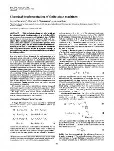
Figure 1: A linear feedback shift register.
q
evolution using a simple replication scheme.
2 REDUNDANT DYNAMIC SYSTEMS
Definition: Let S be a dynamic system with state set QS , input set XS , initial state qs[0], and state evolution qs[t + 1] = �S (qs[t]; xs[t]), where qs [�] 2 QS , xs[�] 2 XS and �S is the next-state function. A dynamic system H with state set QH , input set XH , initial state qh [0], and state evolution equation qh [t + 1] = �H (qh [t]; e(xs[t])) (where e : XS 7?! XH is an injective input encoding) is a redundant implementation for S if it concurrently simulates S in the following sense: there exists a oneto-one state decoding mapping ` : Q0H 7?! QS (where Q0H = `?1(QS ) � QH is the subset of valid states of H) such that
`(�H (`?1 (qs [t]); e(xs[t]))) = �S (qs [t]; xs[t]) for all qs [�] 2 QS , xs[�] 2 XS .
0
in the form (2). Note that when x[�] = 0 and s [0] 6= , this LFSM sequences through all non-zero states. 2 Given a description of the state evolution of an LFSM as in the example above, there are a number of different ways in which it can be implemented in terms of XOR gates and interconnections. In this paper, we assume that each bit in the next-state vector s [t +1] is calculated using a separate set of 2-input XOR gates (as in Figure 1), which implies that a failure in a single XOR gate can corrupt at most one bit in s[t + 1]. Furthermore, we assume that s [t + 1] is calculated based exclusively on the bits of s [t] that are specified by the “1' s” in the matrix of the state evolution equation. It can be shown that any LFSM with state evolution as in eq. (2) can be put in a similar form where the new is in classical canonical form, [2]. What is matrix important about this form is that there are at most two “1' s” in each row of the canonical . This means that each bit in the next-state vector can be generated based on at most two bits of the previous state vector. We now adopt the approach outlined in eq. (1) and look for ways of embedding the given LFSM S into a redundant LFSM H with � state variables (� � d + s, s > 0). The state evolution of H is given by
(1)
2
`?1 (qs [0]) and
If we initialize H to a state qh [0] = encode the input xs [� ] using the encoding mapping e, then under fault-free conditions the state of S at all discrete-time steps � � 0 can be recovered from the state of H through the decoding mapping `; this can be proved easily by induction. The subset Q0H = fqh0 [�] = `?1 (qs[�]) j 8 qs[�] 2 QS g can be regarded as the subset of valid states; detecting a state outside Q0H implies that an error has taken place. Our fault-tolerant scheme consists of a redundant implementation (which takes transitions to possibly corrupted states) and an external mechanism that performs error detection/correction at the end of each time step.
3 FAULT-TOLERANT LFSM's Linear finite state machines (LFSM' s) form a very general class of finite state machines with a variety of applications, including sequence enumerators, encoders and decoders for linear error-correcting codes, and cellular automata. An LFSM S has state evolution
qs[t + 1] = Aqs[t] � Bx[t] ; (2) where t is the discrete-time index, qs [t] is the state vector and x[t] is the input vector. We assume that the vector qs[�] is d-dimensional, x[�] is u-dimensional (operation � denotes vector addition modulo-2).
Example 1: The linear feedback shift register in Figure 1 is implemented using memory elements (flip-flops) and XOR gates (which perform addition modulo-2 and are denoted by � in the figure). The state evolution equation of the shift register in Figure 1 is easily written down
q
A
q
q
A
A
qh [t + 1] = Aqh [t] � Bx[t] ; (3) where matrices A, B are chosen so that qh [t] provides complete information about qs [t] through a decoding
mapping and vice-versa. We will restrict ourselves to techniques that are linear in GF (2); specifically, we assume that there exists (i) a d � � binary full-rank decoding matrix , so that s [t] = h [t] for all t, and (ii) an � � d binary encoding full-rank matrix , so that h [t] = s [t] for all t. The redundant machine H enforces what is termed an (�; d) linear code on the state of the original machine, [3, 4]. The d-dimensional vector s is uniquely represented by the �-dimensional codeword h = s. Under faultfree conditions, the redundant state vector must be in the column space of ; to detect faults, check at each step t that h [t] lies in the column space of , i.e., check that h [t] is a valid codeword. Equivalently, we can check that h [t] is in the null space of an appropriate parity check matrix , so that h [t] = . The proof of the following theorem uses similar techniques as the corresponding theorem in [5]. Theorem 1: In the setting described above, LFSM H is a redundant implementation of S if and only if it is similar to a standard redundant LFSM H� with state evolution
L
q
q
Lq
G
Gq
q
q q q
q
Gq
G
P
G
Pq
�
0
�
�
�
q� [t] � B0 x[t] : (4) (Specifically, there exists an invertible matrix T such that qh [t] = T q� [t] that transforms system H to the above q� [t + 1] = A0 A A
12 22
standard form.) Given a pair of encoding and decoding matrices and (they need to satisfy = d ) and an LFSM S , the
G
LG I
L
above theorem completely characterizes all possible redundant LFSM' s H. Since the choice of the binary matrices 12 and 22 is completely free, there are multiple redundant LFSM' s for S (with the given and ). Example 2: Suppose that the original LFSM S that we would like to protect is the linear feedback shift register shown in Figure 1. In order to detect single errors in an XOR gate, we can use an extra “checksum” state variable (as was suggested in [6, 7, 8]). The resulting redundant LFSM H has six state variables and state evolution
A
A
L
G
� A 0� � b � qh [t + 1] = cT A 0 qh[t] � cT b x[t] ; � � where cT = 1 1 1 1 1 . Under fault-free con-
ditions, the added state variable is always the sum of all other state variables (which remain the same as the original state variables in LFSM S ). The above approach is easily seen to be consistent with our setup. If we use the transformation � [t] =
q �I 0� T qh [t], T = cT 1 , we can show that LFSM H is similar to H� with state evolution � � � � q� [t + 1] = A0 00 q� [t] � b0 x[t] : Note that both A and A are set to zero. There are 5
12
22
multiple redundant implementations with the same encoding, decoding, and parity check matrices. Another choice would have been to set 12 = and 22 = [1], and use the same transformation ( � [t] = T 0h [t]) to get a redundant LFSM H0 with state evolution equation
A
qh0 [t + 1] =
h
0
q
A q
i h b i A 0 q 0 [ t ] � h cT b x[t] : cT A ? A cT A 22
22
Both redundant LFSM' s H and H0 have the same encoding, decoding and parity check matrices and are able to concurrently detect a failure in a single XOR gate (which results in a single-bit error in the state vector). However, the added complexity in H0 is lower than in H, requiring 2 fewer XOR gates. 2
4 UNRELIABLE CORRECTION We assume now that voters fail with probability pv and XOR gates fail with probability px . For simplicity, we assume that there are no failures in the memory elements. To deal with this situation, we use low density parity check (LDPC) codes (see [9, 10]) which can be decoded (corrected) using majority voters and 2-input XOR gates.
4.1 LDPC Codes and Stable Memories
G
with An LDPC code has an n � k generator matrix full-column rank; the additional requirement is that its parity check matrix is (generally sparse and) has exactly K “1' s” in each row and J “1' s” in each column. Each bit in the codeword is involved in J parity checks, each of which involves K ? 1 other bits. Note that the rows of are allowed to be linearly dependent (i.e.,
P
P
P
does not necessarily have n?k rows) and that the generator matrix of an LDPC code is not necessarily sparse. In his seminal thesis [9], Gallager studied ways to construct and decode LDPC codes. In particular, he J constructed (n; k) LDPC codes with rate nk � 1 ? K for fixed J; K . Furthermore, he suggested and analyzed the performance of simple iterative decoding procedures for correcting codeword corruptions. Building on Gallager' s work, Taylor considered how to construct stable (reliable) memories. A stable memory uses n unreliable flip-flops to store k bits of information encoded in an (n; k ) LDPC code; at the end of each time step, an error correction mechanism re-enforces the correct state in the memory; the memory array performs reliably for L time steps if at any given step � � L, the k information bits can be obtained from the n memory bits, i.e., if the codeword stored in the memory after � < L is within the set of n-bit arrays that get decoded to the originally stored codeword. Taylor used Gallager' s (modified) iterative procedure and analyzed its performance using a correction mechanism build out of 2-input XOR gates and (J ? 1)-bit voters (that fail with probability px and pv , respectively). He showed that this iterative decoding scheme can be used to construct reliable memories usJ ) (where J < K ). ing (n; k) LDPC codes ( nk � 1 ? K The larger n is, the less the probability of error for a specified time interval. Note that Taylor' s construction of reliable memories uses J n voters, J n flip-flops, and J n[1 + (J ? 1)(K ? 1)] 2-input XOR gates; one can easily see that the hardware overhead per bit is constant. Taylor also showed that one can reliably perform the component-wise XOR operation on k bits by performing the XOR operation on any two (n; k) codewords. In fact, he showed that one can perform reliably a sequence of � such component-wise XOR operations, [11]. His results for general computation were in error; see the discussions in [12].
G
4.2 Constructing Reliable LFSM's Without loss of generality, we assume that the LFSM S that we are trying to protect has state evolution as in eq. (2) where matrix is in classical canonical form; for simplicity we assume that the input is one-dimensional. We will let k such systems run in parallel (each with distinct input sequence) and then use an LDPC coding scheme to protect these k systems
A
2 qT [t + 1] 3T 66 qT [t + 1] 77 4 .. 5 1
2
. T t k
q [ + 1]
=
2 qT [t] 3T 2 x [t] 3T x [t] 6 qT [t] 7 A 64 .. 75 � b 64 .. 75 1
1
2
2
q []
G
:
. xk t
. T t k
[]
Let be the n � k encoding matrix of an LDPC code. If we post-multiply both sides of the above equation by T we get the following encoded parallel simulations:
G 2 �T [t + 1] 3T 2 �T [t] 3T 02 x [t] 3T 1 66 �T [t + 1] 77 = A 66 �T [t] 77 � b BB6 x [t] 7 GT CC : 4 .. 5 @4 .. 5 A 4 .. 5 1
1
1
2
2
2
. T t �n
[ + 1]
. T t �n
[]
. xk t
[]
Effectively, we have n LFSM' s with state evolution of the form of eq. (2), performing k different encoded simulations of system S . The n replicas receive an encoded version of the k original inputs. We consider the overall simulation to be reliable at a certain time step if the overall state (the state of all n systems) correctly represents the state of the k underlying systems. We will say that the initial failure takes place at step L if L is the earliest time at which the simulation fails. We will show that we can make the probability of such state evolution failure as small as we want; therefore, in order to obtain the underlying system state we mainly incur the fixed probability of failure of the decoding mechanism (which depends on the reliability of the decoding mechanism and not on the way the dynamic system evolves in time). Theorem 2: Let J = 2j , j = 2; 3; 4; :::, K > J . Suppose one can find p < 1=2, J , K such that p >
� J ?1 � J=2
[(K
? 1)(2p + 3px )]J=
2
+ p v + px .
Then,
there exists an (n; k) LDPC (with K “1' s” in each row and J “1' s” in each column of its parity check matrix , J ) such that the probability that the and with nk � 1 ? K initial failure takes place at step L is bounded above by
P
? ; Pr[ initial state evolution failure at step L ] < LdCk
=
?
C q
=
(1
log
� J? (
1)(K
J ?J=K )3 q
2p + 3px
=
h
:
?1)
?
J?2 J=2 ? 1
[(
q J= ?
1) ]
?1)(K ?1)] i?( +3) ? 2J (K1 ?1) ;
2 log[(J
1 2K
� K?
2 1
?3 ;
1 The code redundancy is nk � 1?J=K and the hardware used (including the error correcting mechanism) J ?1)(K ?1)) is bounded below by Jd (3+(1? XOR gates and J=K Jd voters per system. 2 1?J=K
Proof: The proof follows from the proof of [13, 11]. Due to space limitations, we simply outline the proof here. The state of our overall simulations at step t is captured by d codewords Ci [t] (1 � i � d) drawn from an (n; k ) LDPC code; more specifically, the state evolution equation can be written as:
2 C [t + 1] 3 66 C [t + 1] 77 4 .. 5 1
2
.
Cd [t + 1]
2 C [t] 3 6 C [t] 7 A 64 .. 75 � b � X [t] � ; 1
=
2
.
Cd [t]
where X [t] is the encoding of the k inputs. Taylor showed that adding any two such codewords modulo-2 can be done reliably. We use his error correcting mechanism and, during each time step, we allow our system to calculate its new overall state (d new codewords) by adding the codewords of the current state modulo-2. Because matrix is in canonical form, each codeword in the next overall state is created based on at most two codewords of the current state (plus the input modulo-2). So, at each time step we essentially have d
A
additions modulo-2 of the form that Taylor considered. The input is also something that we need to consider (and one of the reasons that our constants differ slightly from Taylor' s) but it is not crucial in the proof since no memory or error propagation is involved in it. 2 Note that our approach can also handle flip-flop failures (for simplicity, our proof assumed no failures). Also, in our construction we did not deal with the encoding function or the cost associated with it. Encoding an LDPC code can be done in a straightforward way if we use the encoding matrix : each of the n redundant bits is generated based on at most k information bits and at most k ? 1 2-input XOR gates. In our approach, however, this is a problem because we let n (and k) increase in order to achieve a smaller probability of failure.
G
References [1] J. von Neumann, Probabilistic Logics and the Synthesis of Reliable Organisms from Unreliable Components. Princeton University Press, 1956. [2] T. L. Booth, Sequential Machines and Automata Theory. New York: Wiley, 1968. [3] W. W. Peterson and E. J. Weldon Jr., Error-Correcting Codes. Cambridge, Massachusetts: The MIT Press, 1972. [4] R. E. Blahut, Theory and Practice of Data Transmission Codes. Reading, Massachusetts: Addison-Wesley, 1983. [5] C. N. Hadjicostis and G. C. Verghese, “Structured redundancy for fault tolerance in LTI state-space models and Petri nets,” Kybernetika, 1999. To appear. [6] K.-H. Huang and J. A. Abraham, “Algorithm-based fault tolerance for matrix operations,” IEEE Transactions on Computers, vol. 33, pp. 518–528, June 1984. [7] A. Chatterjee and M. d' Abreu, “The design of faulttolerant linear digital state variable systems: theory and techniques,” IEEE Transactions on Computers, vol. 42, pp. 794–808, July 1993. [8] R. W. Larsen and I. S. Reed, “Redundancy by coding versus redundancy by replication for failure-tolerant sequential circuits,” IEEE Transactions on Computers, vol. C21, pp. 130–137, February 1972. [9] R. G. Gallager, Low-Density Parity Check Codes. MIT Press, 1963. [10] D. A. Spielman, “Linear-time encodable and decodable error-correcting codes,” IEEE Transactions on Information Theory, vol. 42, pp. 1723–1731, November 1996. [11] M. G. Taylor, “Reliable computation in computing systems designed from unreliable components,” The Bell System Journal, vol. 47, pp. 2239–2366, December 1968. [12] N. Pippenger, “Developments in the synthesis of reliable organisms from unreliable components,” in Proceedings of Symposia in Pure Mathematics, vol. 50, 1990. [13] M. G. Taylor, “Reliable information storage in memories designed from unreliable components,” The Bell System Journal, vol. 47, pp. 2299–2337, December 1968.