Fault-Tolerant Metric Dimension of Graphs∗ Carmen Hernando
(a)
, Merce Mora
(b)
, Peter J. Slater
(c)
, David R. Wood
(b)
(a)
Departament de Matem`atica Aplicada I Universitat Polit`ecnica de Catalunya, Barcelona. Spain
[email protected] (b) Departament de Matem`atica Aplicada II Universitat Polit`ecnica de Catalunya, Barcelona. Spain
[email protected],
[email protected] (c) Mathematical Sciences Dept. and Computer Sciences Dept. University of Alabama in Huntsville. Huntsville. AL, USA 35899
[email protected],
[email protected]
Abstract An ordered set S of vertices in a graph G is said to resolve G if every vertex in G is uniquely determined by its vector of distances to the vertices in S. The metric dimension of G is the minimum cardinality of a resolving set of G. In this paper we introduce the study of the fault-tolerant metric dimension of a graph. A resolving set S for G is fault-tolerant if S \ {v} is also a resolving set, for each v in S, and the fault-tolerant metric dimension of G is the minimum cardinality of such a set. In this paper we characterize the fault-tolerant resolving sets in a tree T . We show that the fault-tolerant metric dimension values are bounded by a function of the metric dimension values independent of any graphs.
1
Introduction
For a graph G with vertex set V (G) and edge set E(G), the distance between two vertices u and v in V (G) is the minimum number of edges in a u − v path and is denoted by dG (u, v) or simply d(u, v) if the graph G is clear. A vertex x resolves two vertices u and v if d(x, u) 6= d(x, v). A vertex set S ⊆ V (G) is said to be resolving for G if for every two distinct vertices u and v in V (G) there is a vertex x in S that resolves u and v. The minimum cardinality of a resolving set of G is called the metric dimension of G and is denoted by β(G). A resolving set of order β(G) is called a metric basis of G. ∗
Research supported by the projects MCYT-FEDER-BFM2003-00368, Gen-Cat-2001SGR00224, MCYT-HU2002-0010, MEC-SB2003-0270, MCYT-FEDER BFM2003-00368. The research of David Wood is supported by a Marie Curie Fellowship of the European Community under contract 023865.
1
Equivalently, for an ordered subset S = (v1 , v2 , . . . , vk ) of vertices in V (G) the S-coordinates of a vertex x in V (G) are fS (x) = (d(x, v1 ), d(x, v2 ), . . . , d(x, vk )). Then S is a resolving set if for every two vertices x and y in V (G) we have fS (x) 6= fS (y). These concepts were introduced for general graphs independently by Slater [6] and by Harary and Melter [4]. Resolving sets have since been widely investigated. (See the bibliographies of [1] and [3].) As described in Slater [6], each vi in S can be thought of as the site for a sonar or loran station, and each vertex location must be uniquely determined by its distances to the sites in S. In this paper we consider (single) fault-tolerant resolving sets S for which the failure of any single station at vertex location v in S leaves us with a set that still is a resolving set. A resolving set S for a graph G is fault-tolerant if S \ {v} is also resolving for each v in S. The fault-tolerant metric dimension of G is the minimum cardinality of a fault-tolerant resolving set, and it will be denoted by β 0 (G). A fault-tolerant resolving set of order β 0 (G) is called a fault-tolerant metric basis. We consider fault-tolerant resolving sets for trees in section 2. In section 3 we show that the fault-tolerant metric dimension values are bounded by a function of the metric dimension values independent of any given graph.
2
Fault-tolerant resolving sets for trees
Consider the tree T 0 in Figure 1. It will be seen below that β(T 0 ) = 10 and that S = (1, 2, . . . , 10) is a metric basis. We have, for example, that fS (x) = (11, 11, 11, 11, 10, 10, 10, 10, 1, 4) , fS (y) = (11, 11, 11, 11, 10, 10, 10, 10, 3, 4) , fS (v) = (8, 8, 8, 8, 3, 3, 7, 7, 8, 9) , fS (t) = (8, 8, 8, 8, 1, 3, 7, 7, 8, 9) . Note that fS (x) and fS (y) agree everywhere except for the ninth component, that is, the only vertex in S that resolves vertices x and y is vertex 9. Likewise, only vertex 5 resolves vertices v and t. We will see that β 0 (T 0 ) = 14 and that S ∪ {y, v, r, s} is one example of a fault-tolerant metric basis of T 0 . It is easy to see that for the path Pn on n ≥ 2 vertices we have β(Pn ) = 1 and β 0 (Pn ) = 2. Observe that the unique fault-tolerant metric basis of Pn is formed by the two endpoints. Henceforth we will only be concerned with trees T that have maximum degree ∆(T ) ≥ 3. The degree of vertex v is denoted by deg(v). 2
T0 10
x
y
6
w
9
z
u
s1
v
t s3
s2
s4
5
s5
s6
8 1
7
2
3
4
s
r
Figure 1: Tree T 0 with β(T 0 )=10 and β 0 (T 0 ) = 14 A branch of a tree T at a vertex v is the subgraph induced by v and one of the components of T \ {v}. Note that each v ∈ V (T ) has deg(v) branches. A branch B of T at v which is a path will be called a branch path when deg(v) ≥ 3. Tree T 0 (see Figure 1) has sixteen branch paths. The vertex v in a branch path with deg(v) ≥ 3 will be called a stem of the branch path. Tree T 0 has six stems: s1 , . . . , s6 . We let L1 , . . . , Lk be the components of the subtree induced by the set of all branch paths. Thus k is the number of stems, and each Li can be obtained by subdividing edges starting with a star. For T 0 we have k = 6 and subdivisions: one K1,5 , three K1,3 and two K1,1 . Theorem 2.1 ([6]) Let T be a tree of order n ≥ 3. Vertex set S is a resolving set if and only if for each vertex u there are vertices from S on at least deg(u) − 1 of the deg(u) components of T \ {u}. Theorem 2.2 ([6]) Let T be a tree with set L of endpoints with |L| ≥ 3. Let L1 , . . . , Lk be the components of the subtree induced by the set of all branch paths, and let ei be the number of branch paths in T that are in Li . Then β(T ) = |L| − k, and S is a metric basis if and only if it consists of exactly one vertex from each of exactly ei − 1 of the branch paths of Li , for each Li , 1 ≤ i ≤ k. Assume that S is a fault-tolerant resolving set for tree T . For each v in S, the set S \ {v} is a resolving set. By Theorem 2.1, for any v ∈ S ∩ Li , the set S \ {v} must contain 3
a vertex from each of ei − 1 of the branch paths of Li . Thus, |S ∩ Li| ≥ ei when ei ≥ 2. If L is the set of endpoints and E1 is the set of endpoints to branch paths where ei = 1, then, by Theorem 2.1 , L \ E1 is a fault-tolerant resolving set. This implies the next theorem. Theorem 2.3 Let T be a tree with set L of endpoints with |L| ≥ 3. Let L1 , . . . , Lk be the components of the subtree induced by the set of all branch paths, and let ei be the number of branch paths in T that are in Li . Let E1 be the set of endpoints corresponding to branch paths where ei = 1. Then β 0 (T ) = |L \ E1 | and L \ E1 is a fault-tolerant metric basis. Remark 2.4 If S is a fault-tolerant metric basis for T and si is the stem vertex of Li , then ei ≥ 3 implies that S ∩Li will consist of exactly one vertex from each path of Li \{si }, and, if ei = 2, then S ∩ Li can be any two vertices of Li \ {si }. In particular, for the tree T 0 of Figure 1, β 0 (T 0 ) = 14 and (1, 2, 3, . . . , 10, y, v, r, s) is one example of a fault-tolerant metric basis.
3
Relation between β 0 (G) and β(G).
In this section we prove that fault-tolerant metric dimension is bounded by a function of metric dimension (independent of the graph). As usual, N (v) and N [v] denote vertex v’s open and closed neighborhoods, respectively. Lemma 3.1 Let S be a resolving set of G. For each vertex v ∈ S, let T (v) := {x ∈ V (G) : N (v) ⊆ N (x)}. Then S 0 := ∪v∈S (N [v] ∪ T (v)) is a fault-tolerant resolving set of G. Proof. Consider a vertex v ∈ S 0 . If v 6∈ S then S 0 \ {v} resolves G since S ⊆ S 0 \ {v}. Now assume that v ∈ S. Let p and q be distinct vertices of G. We must show that p and q are resolved by some vertex in S 0 \ {v}. If not, then v must resolve p and q since S resolves p and q. Without loss of generality d(v, p) ≤ d(v, q) − 1. First suppose that p 6= v. Let w be the neighbour of v on a shortest path between v and p. Then w ∈ S 0 \ {v} and d(v, p) = d(w, p) + 1. Thus d(w, p) + 1 ≤ d(v, q) − 1. Now d(v, q) − 1 ≤ d(w, q). Hence d(w, p) + 1 ≤ d(w, q). Thus w resolves p and q. Now assume that p = v. If q ∈ S 0 then q ∈ S 0 \ {v} and q resolves p and q. Otherwise d(v, q) ≥ 2 and q is not adjacent to some neighbour w of v. Then d(v, w) = 1 and d(q, w) ≥ 2. Thus w ∈ S 0 \ {v} resolves v (= p) and q. Hence S 0 is a fault-tolerant resolving set of G. The following lemma is implicit in [2, 5]. We include the proof for completeness. 4
2
Lemma 3.2 Let S be a resolving set in a graph G. Then for each vertex v ∈ S, the number of vertices of G at distance at most k from v is at most 1 + k(2k + 1)|S|−1 . Proof. Say 1 ≤ d(v, w) ≤ k. For every vertex u ∈ S with u 6= v, we have |d(w, u) − d(w, v)| ≤ k. Thus there are 2k + 1 possible values for d(w, u), and there are at most k possible values for d(w, v). Thus the vector of distances from w to S has k(2k + 1)|S|−1 possible values. The result follows, since the vertices at distance at most k are resolved by S. 2 Theorem 3.3 Fault-tolerant metric dimension is bounded by a function of the metric dimension (independent of the graph). In particular, β 0 (G) ≤ β(G)(1 + 2 · 5β(G)−1 ) for every graph G. Proof. Let S be a metric basis for a graph G. Lemma 3.2 with k = 2 implies that |N [v] ∪ T (v)| ≤ 1 + 2 · 5β(G)−1 for each vertex v ∈ S. Thus |S 0 | ≤ β(G)(1 + 2 · 5β(G)−1 ). 2
References [1] Jos´e C´aceres, Carmen Hernando, Merc`e Mora, Ignacio M. Pelayo, Mar´ia L. Puertas, Carlos Seara, and David R. Wood. On the metric dimension of cartesian products of graphs. SIAM J. Discrete Math., to appear. http://www.arxiv.org/math/0507527. [2] Gary Chartrand, Linda Eroh, Mark A. Johnson and Ortrud R. Oellermann . Resolvability in graphs and the metric dimension of a graph. Discrete Appl. Math., 105(1-3): 99–113, 2000. [3] Gary Chartrand and Ping Zhang. The theory and applications of resolvability in graphs. A survey. Proc. 34th Southeastern International Conf. on Combinatorics, Graph Theory and Computing, vol. 160 of Congr. Numer.: 47–68, 2003. [4] Frank Harary and Robert A. Melter. On the metric dimension of a graph. Ars Combinatoria, 2: 191–195, 1976. [5] Samir Khuller, Balaji Raghavachari and Azriel Rosenfeld. Landmarks in graphs. Discrete Appl. Math., 70(3): 217–229, 1996. [6] Peter J. Slater. Leaves of trees. Proc. 6th Southeastern Conf. on Combinatorics, Graph Theory, and Computing, vol. 14 of Congressus Numerantium: 549–559, 1975.
5