pose tracking over a wider range of velocity due to increased precision of ICP ..... −0.05. 0. 0.05. 0.1. Time (s). ˙ ˆr. (m/s) ω. (rad/s). ˙rx. ˙ry. ˙rz ωx ωy ωz. Fig. 5.
2010 IEEE/ASME International Conference on Advanced Intelligent Mechatronics Montréal, Canada, July 6-9, 2010
Fault-tolerant Pose Estimation of Space Objects Farhad Aghili∗ , Marcin Kuryllo† , Galina Okouneva† and Chad English‡ ∗
†
Space Technologies, Canadian Space Agency Saint-Hubert, Quebec, Canada J3Y 8Y9 Department of Aerospace Engineering, Ryerson University Toronto, Ontario, Canada M5B 2K3 ‡ Neptec Design Group, Director of R&D Kanata, Ontario, Canada K2K 1Y5
Abstract—This paper presents a fault-tolerant method for pose estimation of space objects using 3-D vision data by integration of a Kalman filter (KF) and an Iterative Closest Point (ICP) algorithm in a closed-loop configuration. The initial guess for the internal ICP iteration is provided by state estimate propagation of the Kalman filer. The Kalman filter is capable of not only estimating the target’s states, but also its inertial parameters. This allows the motion of target to be predictable as soon as the filter converges. Consequently, the ICP can maintain pose tracking over a wider range of velocity due to increased precision of ICP initialization. Furthermore, incorporation of the target’s dynamics model in the estimation process allows the estimator continuously provide pose estimation even when the sensor temporally loses its signal namely due to obstruction. The capabilities of the pose estimation methodology is demonstrated by a ground testbed for Automated Rendezvous & Docking (AR&D).
I. I NTRODUCTION There are several on-orbit servicing missions in the horizon that will require capabilities for autonomous rendezvous & docking, autonomous rendezvous & capture, proximity operation of space vehicles, constellation satellites, and formation flying [1]–[3]. Successful accomplishment of these mission critically relies on a fault-tolerant sensor system to obtain real-time relative pose information (in 6-dof) of two spacecraft during proximity operation. There are different vision systems capable of estimating the pose (position and orientation) of moving objects. However, among them, an active vision system such as Neptec Laser Camera System (LCS) is preferable because of its robustness in face of the harsh lighting conditions of space [4]. As verified during the STS-105 space mission, the 3D imaging technology used in the LCS can indeed operate in space environment. The use of laser range data has also been proposed for the motion estimation of free-floating space objects [5]. All vision systems, however, provide discrete and noisy pose data at relatively low rate, which is typically 1 Hz. It is worth mentioning that another 3D sensor system called TriDAR is an emerging technology that combines the complementary nature of LCS triangulation and Lidar time-of-flight for enhancing the scan range [6]. Taking advantage of the simple dynamics of a free-floating object, which is not acted upon by any external force or moment, researchers have employed different observers to
978-1-4244-8030-2/10/$26.00 ©2010 Crown
track and predict the motion of a target satellite [7]–[9]. Using the the Iterative Recursive Least Squares pose refinement [10], the visual information from camera has been used for relative pose estimation for autonomous rendezvous & docking [11]. In some circumstances, e.g., when there are occlusions, no sensor data is available. Therefore, prediction of the motion of the target based on the latest estimation of its states and dynamic parameters are needed for a continuous pose estimation. This work is focused on the integration of the Kalman filter and the ICP algorithm in a closed-loop configuration for accurate and fault-tolerant pose estimation of a freefalling tumbling satellite. In the conventional pose estimation algorithm, the range data from a rangefinder scanner along with a CAD-generated surface model are used by the ICP algorithm to estimate the target’s pose. The estimation can be made more robust by placing the ICP algorithm and the KF estimator in a closed-loop configuration, wherein the initial guess for the ICP is provided by the estimate prediction. The pose estimation based on the ICP-KF configuration has the following advantages: i) The KF reduced the measurement noise, thus providing a more precise pose estimation. ii) Faster convergence of the ICP iteration and maintaining tracking over a wider range of object velocity are achieved as a consequence of increased precision of the ICP initial guess provided by KF. iii) Continuous pose estimation becomes possible even in the presence of temporary sensor failure or obstruction as a consequence of incorporation of the dynamic model of the target in the estimation process. The KF estimator is designed so that it can estimate not only the target’s states, but also its dynamic parameters. Specifically, the dynamic parameters are the ratios of the moments of inertia of the target, the location of its center of mass, and the orientation of its principal axes. Not only does this allow long-term prediction of the motion of the target, which is needed for motion planning, but also it provides accurate pose feedback for the control system when there are blackout, i.e., no observation data are available. In this work, we use the Euler-Hill equations [12] to derive a discrete-time
947
model that captures the evolution of the relative translational motion of a tumbling target satellite with respect to a chaser satellite which is freely falling in a nearby orbit. II. ICP A LGORITHM This section reviews the basic ICP algorithm originally proposed by Besl and McKay [13]. The ICP algorithm is an iterative procedure which minimizes a distance between point cloud in one dataset and the closest points in the other. Suppose that we are given with a set of 3-D point cloud data U = {u1 · · · um } that corresponds to a single shape represented by model set M. It is known that for each point ui ∈ R3 from the 3-D points data set U, there exists at least one point, vi , on the surface of M which is closer to ui than other points in M [14]. The ICP algorithm assumes that the initial rigid transformation {A0 , r0 } between sets U and M is known; r0 and A0 denote the translation vector and the rotation matrix, respectively. Then, the problem of finding the correspondence between the two sets can be formally expressed by vi = arg min �A0 ui + r0 − vj � vj ∈M
∀i = 1, · · · , m, (1)
and then set V = {v1 · · · vm } is formed accordingly. Now, we have two independent sets of 3-D points V and U both of which corresponds to a single shape. The problem is to find a fine alignment {A, r} which minimizes the distance between these two sets of points [13]. This can be formally stated as m
1 � �Aui + r − vi �2 d =arg min r,A m i=1
∀vi ∈ V, ui ∈ U (2)
s.t.
T
A A = 13
There are several closed-form solutions to the above leastsquares minimization problem [15], [16], of which the quaternion-based algorithm [17] is the preferable choice for m > 3 over other methods [13]. The rotation matrix can be written as a function of unit quaternion as A(q) = (2qo2 − 1)13 + 2qo [qv ×] + 2qv qvT .
(3)
where qv and qo are the vector and scaler parts of the quaternion, i.e., q = [qvT qo ]T . Consider the cross-covariance matrix of the sets V and U given by 1 � ¯T vi uTi − v¯u (4) S = cov(V, U) = m i where v¯ =
1 � vi m i
¯= and u
1 � ui m i
(5)
are the corresponding centroids of the sets. Then, it can be shown that minimization problem (2) is tantamount to find the solution of following quadratic programming [17] T
max q W q
�q�=1
(6)
where the symmetric weighting matrix W can be constructed from cross-covariance matrix, S, as follow ⎡ s11 + s22 + s33 × × ⎢ s23 − s32 s11 − s22 − s33 × ⎢ W =⎣ s31 − s13 s21 + s12 −s11 + s22 − s33 s12 − s21 s31 + s13 s23 + s32 ⎤ ··· × ⎥ ··· × ⎥ (7) ⎦ ··· × · · · −s11 − s22 + s33 where sij denotes the ijth entry of matrix S. The unit ˘ that maximizes the quadratic function of (6) quaternion, q, is the eigenvector ξi corresponding to the largest eigenvalue of the matrix W , i.e., q˘ = ξi (W ) so that λi (W ) = λmax . Then, the translation can be obtained from ˘u ¯ r˘ = v¯ − A(q)
(8)
The ICP-based matching algorithm may proceed through the following steps: i) Given an initial coarse alignment {q0 , r0 }, find closest point pairs V from scan 3-D points set U and model set M according to (1). ˘ r˘} miniii) Calculate the fine alignment translation {q, mizing the mean square error the distance between two data sets U and V according to (6)-(8) iii) Apply the incremental transformation from step ii to step i. iv) Iterate until either the residual error d is less than a threshold, dmin , or the maximum number of iteration is reached. It has been shown that the above ICP algorithm is guaranteed to converge to a local minimum [13]. However, a convergence to a global minimum depends on a good initial alignment [18]. In pose estimation of moving objects, “good” initial poses should be provided at the beginning of every ICP iteration. The initial guess for the pose can be taken from the previous estimated pose obtained from the ICP [4]. However, this can make the estimation process fragile when dealing with relatively fast moving target. This is because, if the ICP does not converge for a particular pose, e.g., due to occlusion, in the next estimation step, the initial guess of the pose may be too far form its actual value. If the initial pose happens to be outside the global convergence region of the ICP process, from that point on, the pose tracking is most likely lost for good. The estimation can be made more robust by placing the ICP and a dynamic estimator in a closed-loop configuration, whereby the initial guess for the ICP is provided by the estimate prediction of the moving object. The following sections described design of a Kalman filter which will be capable of not only estimating the states but also and parameters of a free-floating object. III. M OTION DYNAMICS Fig. 1 illustrates the chaser and the target satellites as rigid bodies moving in nearby orbits. Coordinate frames {A} and {B} are attached to the chaser and the target, respectively.
948
observing satellite
target satellite
ω
{A} x Camera
y
CM
POR
r rc
{B}
{C}
ρ
CM
Fig. 1. The body-diagram of chaser and target satellites moving in neighboring orbits
The origins of frames {A} and {B} are located at centerof-masses (CM)s of the observing and target satellites. The axes of {B} are chosen to be parallel to the principal axes of the target satellite, while {A} is orientated so that its x-axis is parallel to a line connecting the Earth’s center to the chaser CM and pointing outward, and its y-axis lies on the orbital plane; see Fig. 1. The coordinate frame {C} is fixed to the target at its point of reference (POR) located at distance ρ from the origin of {B}. It is the pose of {C} that is measured by the laser camera. We further assume that the target satellite tumbles with angular velocity ω. Also, notice that the coordinate frame {A} is not inertial; rather, it moves with the chaser satellite. Below, vectors ρ and ω are expressed in {B}. We choose to express the target orientation in the bodyattached frames coincident with its principal axes, {B}, while the translational motion variables are expressed in the body attached frame of the chaser, {A}. The advantages of such a mixed coordinate selection are twofold: Firstly, the inertia matrix becomes diagonal and will be independent of the target orientation, thus resulting in a simple attitude model. Secondly, choosing to express the relative translational motion dynamics in {A} leads to decoupled translational and rotational dynamics that greatly contributes to the simplification of the mathematical model; note that, since {B} is a rotating frame, the translational acceleration seen from this frame depends on both the relative angular velocity and relative acceleration. In the following, subscripts r and t denote quantities associated with the rotational and translational dynamics of the system, respectively. A. Review of Quaternion Kinematic In this section, we review some basic definitions and properties of quaternions used in the rest of the paper. Consider quaternions q1 , q2 , q3 and their corresponding rotation matrices A1 , A2 , and A3 , respectively. Operators ⊗ and � are defined as
−[qv ×] + qo 13 qv [qv ×] + qo 13 qv [q⊗] � , [q�] � −qvT qo −qvT qo (9) where [qv ×] is the cross-product matrix of qv . Then, q3 = q1 � q2 ≡ q2 ⊗ q1 corresponds to product A3 = A1 A2 .
Also, the conjugate quaternion 1 q ∗ of q is defined such that q ∗ ⊗ q = q ⊗ q ∗ = [0 0 0 1]T . Moreover, both ⊗ and � operations have associative property, hence q1 ⊗ q2 ⊗ q3 and q1 � q2 � q3 being unambiguous. The orientation of {A} with respect to {C} is represented by the unit quaternion q, while the orientation of {A} with respect to {B} is represented by the unit quaternion μ. Moreover, η is a constant unit quaternion which represent orientation of the principal axes, i.e., orientation of {B} with respect to {C}. Therefore, the following kinematic relation holds among the aforementioned quaternions q = η ⊗ μ.
(10)
B. State Equations In the rest of this paper, the underlined form of any vector a ∈ R3 denotes the representation of that vector in R4 , e.g., aT � [aT 0]. Recall that the orientation of the principal axis of the target satellite with respect to the chaser satellite is represented by a unit quaternion μ. The time derivative of μ and the relative angular velocity ωrel are related by μ˙ =
1 ω ⊗ μ, 2 rel
where
ωrel = ω − ωn ,
(11)
and ωn is the angular velocity of the chaser satellite expressed in the frame {B}. Assume that the attitude-control system of the chaser satellite makes it rotate with the angular velocity of the reference orbit. Furthermore, denoting the angular velocity of the reference orbit expressed in {A} with � T (12) n≡ 0 0 n , one can relate n and ωn using the quaternion transformation below: ω n = μ ⊗ n ⊗ μ∗ . (13) Substituting (13) into (11) and using the properties of the quaternion products, we arrive at 1 1 ω ⊗ μ − (μ ⊗ n) ⊗ (μ∗ ⊗ μ) 2 2 � 1 = ω ⊗ −n � μ 2
μ˙ =
(14)
Define the variation of actual quaternion, μ, from its nominal ¯ as value, μ, ¯∗ (15) δμ = μ ⊗ μ Then, adopting a technique similar to that used by other authors in [9], [19], we can linearize the time derivative ¯ and ω ¯ to of the above equation about the estimated states μ obtain 1 d ¯ × δμv + δω. δμv ≈ −ω (16) dt 2 Assuming that the spacecraft is acted upon by three independent disturbance torques about its principal axes and
949
1 q∗ o
= qo and qv∗ = −qv .
denoting the principal moments of inertia as Ixx , Iyy , and Izz , we can write Euler’s equations as
by unit quaternion, η, are uncertain. Now assume that the state vector to be estimated is:
Ixx ω˙ x = (Iyy − Izz )ωy ωz + τx , Iyy ω˙ y = (Izz − Ixx )ωz ωx + τy ,
x = [μTv ω T pT rcT r˙ cT ρT ηvT ]T ∈ R21
Izz ω˙ z = (Ixx − Iyy )ωx ωy + τz . Rewriting the above equations in terms of the perturbation �τ = [τx /Ixx τy /Ixx τz /Ixx ]T , we obtain ω˙ = ψ(ω) + J(p)�τ ,
(17)
(22)
where ηv is the vector part of unit quaternion η. One can combine the nonlinear equations (14), (17), (19) in the standard form as x˙ = f (x, �), which can be used for state propagation. However, the KF design also requires the statetransition matrix of the linearized system. Let us define the variation of quaternion η with respect to its nominal value η¯ according to δη= η¯∗ ⊗ η.
where pT = [px py pz ], px = (Iyy − Izz )/Ixx , py = (Izz − Ixx )/Iyy , and pz = (Ixx − Iyy )/Izz are the inertia ratios, and Then setting the linearized equations (16), (18), and (21) in ⎤ ⎡ the standard state-space form yields: px ω y ω z � 1 − py 1 + pz � ⎦ ⎣ , . ψ(ω) = py ωx ωz , J(p) = diag 1, δ x˙ = F δx + B� (23) 1 + px 1 − px pz ω x ω y where vector � = [�Tτ �Tf ]T contains the entire process noise, ¯ and p¯ yields Linearizing (17) about ω and ⎤ ⎡ 1 ¯ p)δω ¯ ¯ ¯ τ, (18) δ ω˙ = M (ω, + N (ω)δp + J(p)� ¯ 03 03 03 03×6 −[ω×] 2 13 ⎢ 03 ¯ p) ¯ N (ω) ¯ M (ω, 03 03 03×6 ⎥ ⎥ ⎢ ⎤ ⎡ ⎢ 03 03 03 03 03×6 ⎥ 0 px ω z px ω y ⎥, ⎢ 03 ∂ψ ⎣ F = ⎢ 03 03 03 03 13 03×6 ⎥ 0 py ω x ⎦ = py ω z M (ω, p) = ⎥ ⎢ ∂ω ⎣ 03 03 03 K(n) −2[n×] 03×6 ⎦ pz ω y pz ω x 0 ⎡ ⎤ 06×3 06×3 06×3 06×3 06×3 06 ω ω 0 0 ∂ψ ⎣ y z ⎦ ⎤ ⎡ = 0 ωx ωz 0 N (ω) = . 03 03 ∂p 0 0 ωx ωy ⎢J(p) ¯ 03 ⎥ ⎥ ⎢ ⎥ 0 0 B=⎢ The evolution of the relative position of the two satellites 6×3 6×3 ⎥ . ⎢ ⎣ 03 13 ⎦ can be described by the Euler-Hill model in orbital mechan06×3 06×3 ics. Let the chaser move on a circular orbit with radius Re , thus the carrier ray having an angular rate n. Further, assume The equivalent discrete-time system (23) can be written as that vector rc denotes the relative position of the CM’s of the two satellites expressed in the frame {A}. Then, the (24) δxk+1 = Φk δxk + wk . translational motion of the target satellite can be expressed Here the solution to the state transition matrix Φk and as � � discrete-time process noise Qk = E[wk wkT ] can be obtained re + rc T +n2 re +�f , based on the van Loan method [22] as Φk = D22 r¨c = −2n×r˙ c −n×(n×rc )+ −μe and �re + rc �3 (19) Qk = Φk D12 , where
� −F BΣB T � where μe is the gravitational parameter of the Earth and re = D11 D12 T D= = exp T [Re 0 0] is a constant position vector expressed in frame 0 D22 0 FT {A} that connects the Earth’s center to the chaser CM, and �f denotes the perturbation of translational motion. Note that the with T being the sampling time and Σ = E[��T ] = constant position vector can be computed from the angular diag{στ2 13 , σf2 13 }. rate of the circular orbit by IV. O BSERVATION E QUATIONS
T � 3 μe The ICP algorithm gives noisy measurements of the posi(20) re = 0 0 . n2 ˘ of the target. In the followings, tion, r˘, and orientation, q, The linearized equations of the translational motion, which the measurement variables will be expressed in terms of the are known as the Euler-Hill equations [20] or the Clohessy- states variables. It is apparent from (1) that Wiltshire equations [21], can be written as (25) r = rc + A(μ)ρ, (21) δ r¨c = K(n)δrc − 2n × δ r˙ c + �f , Also, recall from (10) that quaternion q can be described where K(n) = diag{3n2 0 − n2 }. as a function of η and μ, i.e., q(μ, η) = η ⊗ μ. Consider ¯ which are chosen to be close In addition to the inertia of the target satellite, the location nominal quaternions η¯ and μ of CM, ρ, and the orientation of the principal axis denoted to the actual quaternions; as will be later discussed in the
950
next section. Then, the variation of the quaternion, δq, with respect to nominal quaternions is defined as ¯ ∗ = δη ⊗ δμ. δq = η¯∗ ⊗ q ⊗ μ
(26)
and (ii) estimate propagation � ˆ− ˆ x = x + k k+1 − = Pk+1
Thus, the observation equation can be written as z = h(x) + ν
(27)
where ν is the measurement noise, which is assumed to be white with the covariance E[νν T ] = R, and
r˘ rc + A(δμ ⊗ μ)ρ z= , h(x) = . (28) δ q˘ vec(δη ⊗ δη) Note that the observation vector (28) is a nonlinear function of the states. To linearize the observation vector, one also needs to derive the sensitivity of the nonlinear observation vector with respect to the system states. It can readily be seen from (3) that, for a small rotation δμ, i.e., �δμv � � 1 and δμ0 ≈ 1, the first-order approximation of the rotation matrix can be written as
f (x(t), 0) dt
+ Qk
(32a) (32b)
point cloud dataset refined pose
ICP sensor initial pose unit delay
Hence, (25) can be approximated as (29)
(a) Each ICP iteration uses the last iteration’s pose estimate to seed the next iteration.
¯ = A(μ). ¯ Moreover, in view of the definition of the where A quaternion product and assuming small quaternion variations, we can say that δqv ≈ δμv × δηv + δμv + δηv .
tk Φk Pk ΦTk
The unit quaternions are computed right after the innovation step (31b) from � � ˆ vk δμ 1 �1/2 ⊗ e 2 T [ωˆ k−1 ⊗] μ ˆ k−1 , ˆk = μ 2 ˆ vk � 1 − �δ μ � � δ ηˆvk �1/2 ηˆk−1 . ηˆk = 1 − �ηˆvk �2
A(δμ) ≈ 13 + 2[δμv ×] ¯ + 2δμv × ρ), r ≈ rc + A(ρ
tk+1
(30)
It is apparent from (29) and (30) that the measurement equations are bilinear functions of the states. Consequently, we can derive the sensitivity matrix H = ∂h ∂x as ¯ −2A[ρ×] 03 03 13 03 H= −[δηv ×] + 13 03 03 03 03
¯ 3 + 2[δμv ×]) · · · A(1 03 . ··· 03 [δμv ×] + 13 A. Filter design Recall that δμv is a small deviation from the the nominal ¯ Since the nominal angular velocity ω ¯ k is trajectory μ. assumed constant during each interval, the trajectory of the nominal quaternion can be obtained from 1
¯ k = e 2 T [ωˆ k−1 ⊗ ]μ ˆ k−1 . μ However, since η is a constant variable, we can say η¯k = ηˆk−1 . Let us assume that the sate vector is partitioned as x = [μTv χT ηvT ]T . Then, the EKF-based observer for the associated noisy discrete system (24) is given in two steps: (i) estimate correction
�−1 (31a) Kk = Pk− HkT Hk Pk− HkT + Rk ⎤ ⎡ −⎤ ⎡ ˆ vk δμ ˆ vk δμ �
⎦ + K zk − h(x ⎣ χ ˆk ⎦ = ⎣ χ ˆ− ˆ− (31b) k k) δ ηˆvk δ ηˆv−k �
(31c) Pk = 121 − Kk Hk Pk−
ICP
refined pose
pose estimation
EKF
pose prediction
initial pose
(b) Each ICP iteration uses the KF pose prediction for the time a new dataset is acquired by the sensor. Fig. 2.
Pose tracking of moving objects.
B. ICP-KF Closed-Loop Configuration Fig.2(a) illustrates the conventional ICP loop where each iteration uses the last iteration’s pose estimate to seed the next iteration either for a fixed number of iterations, fixed time limit, or some convergence criteria are met. The refined pose obtained from the ICP algorithm is then considered as the pose estimation. In this configuration, a new dataset is acquired and the output pose from the last dataset is normally used as the initial pose for the new dataset. On the other hand, Fig.2(b) illustrates the ICP and KF in a closed-loop configuration where the refined pose is used as a input to KF while, in turn, the pose prediction of KF is used as the initial pose for the ICP. More specifically, the latter pose estimation process takes the following steps: i) Refine an initial given pose by applying the ICP iteration on a dataset acquired by the laser sensor. ii) Input the refined pose to the KF in order to filter out the sensor noise and to estimate the object velocities as well as its dynamic parameters. iii) Use the estimation of the states and parameters to propagate the pose at the time when a new dataset is acquired by the sensor. iv) Go to step i and use the pose prediction as the initial pose.
951
rˆ˙ (m/s)
0.02
r˙x r˙y r˙z
0.01
0
−0.01 0
20
40
60
80
100
120
140
160
ˆ (rad/s) ω
0.1
(a) The satellite CAD model.
Z (m)
ωx ωy ωz
0.05
0
−0.05 0 −2 −2.2 −2.4 −2.6 −2.8
180
Fig. 5.
20
40
60
80
100
Time (s)
120
140
160
180
Estimations of the satellite’s linear and angular velocities
−0.4 −0.3
3 −0.2
px py pz
2 −0.1
1
0.4 0
pˆ
0.3 0.2
0.1
0.1 0
0.2 −0.1
X (m)
0.3
0
−1 −2
−0.2 −0.3 0.4
−0.4
−3 0
Y (m)
20
40
60
80
100
120
140
160
180
(b) The point-cloud data from scanning of the satellite. 0.1
Fig. 3. Matching points from the CAD model and the scanned data to estimate the satellite pose.
ρx ρy ρz
ρˆ (m)
0 −0.1 −0.2
0
20
40
60
80
100
120
140
160
180
time
Fig. 6. Estimations of the satellite’s dynamics parameters versus their actual values depicted by dotted lines.
6 Satellite mockup
spacecraft simulator that drives the manipulator, parameters are selected as ⎡ ⎤ ⎡ ⎤ 4 0 0 −0.15 Ic = ⎣0 8 0⎦ (kgm2 ) and ρ = ⎣ 0 ⎦ (m). 0 0 5 0
Laser camera sys.
?
Fig. 4.
The experimental setup.
V. E XPERIMENT In this section, experimental results are presented that show comparatively the performance of the pose estimation with and without KF in the loop. Fig. 4 illustrates the experimental setup where a satellite mockup is attached to a manipulator arm, which is driven by a simulator according to orbital dynamics. The Neptec’s laser rangefinder scanner is used to obtain the pose measurements at a rate of 2 Hz. For the
The solid model of the satellite mockup, Fig. 3(a), and the point-cloud data, generated by the laser rangefinder sensor, Fig. 3(b), are used by the ICP algorithm to estimate the satellite’s pose according to the ICP initialization configurations illustrated in Fig. 2. Three test runs conduced to demonstrate the capability of the estimator are: (i) identification of the spacecraft dynamics parameters, (ii) accuracy and robustness of pose tracking at high velocity, (iii) pose tracking in presence of occlusions. A. Identification of Dynamics Parameters Figs. 5 and 6 show the trajectories of the estimated velocities and parameters, respectively. The true values of the parameters are depicted by dotted lines in Fig. 6. It is evident
952
0.3
CL EKF OL EKF
0.9
CL EKF OL EKF
ICP error
rx (m)
ICP
0.85 0.8 0
20
40
60
80
100
0.2
0.1
120
0.38
0 0
ry (m)
20
40
60
Time (s)
0.36 0.34 0.32 0
Fig. 10. 20
40
60
80
100
80
100
120
Normalized ICP fit metric.
120
occlusion
occlusion
0.1
rx (m)
rz (m)
0.05 0
0.9
ICP CL EKF
0.85
−0.05 20
Fig. 7.
40
60
Time (s)
80
100
0.8 0
120
20
40
60
80
100
120
20
40
60
80
100
120
20
40
60
80
100
120
0.38
ry (m)
0
Tracking of the satellite’s position.
0.36 0.34 0
ICP CL EKF OL EKF
0
−200 0
0.1
rz (m)
Yaw (deg)
200
20
40
60
80
100
Roll (deg)
0
120 −0.05 0
40
Time (s)
20
Fig. 11.
Tracking of the satellite’s position in the presence of occlusion.
0 0
Pitch (deg)
0.05
20
40
60
80
100
120
from the graphs that the estimated dynamics parameters converged to their true values after about 120 s.
−60 −80
B. Pose Tracking at high velocity
−100 0
20
Fig. 8.
40
60
Time (s)
80
100
120
Tracking of the satellite’s attitude.
The robustness of the pose estimation of the tumbling satellite with and without incorporating the KF are comparatively illustrated in Figs 7, 8, and 9. Note that here the quaternion is converted to the the Euler’s angles for representing the orientation. It is evident from the figures
0
−0.02
actual CL EKF OL EKF
−0.04 −0.06 0
20
40
60
80
100
120
0
ωy (rad/s)
0.2
20
40
60
80
100
120
20
40
60
80
100
120
20
40
60
80
100
120
Roll (deg)
40
0.1 20
40
60
80
100
120
0.1
ωz (rad/s)
occlusion
ICP CL EKF
−200 0
0 0
occlusion
200
Yaw (deg)
ωx (rad/s)
0.02
20 0 0
0 0
20
40
60
Time (s)
80
100
120
Pitch (deg)
0.05
−60 −80 −100 0
Fig. 9.
Satellite’s angular velocities. Fig. 12.
953
Tracking of the satellite’s attitude in the presence of occlusion.
occlusion
ωx (rad/s)
0.02 0
occlusion
R EFERENCES
actual CL EKF
−0.02 −0.04 −0.06 20
40
60
80
100
120
20
40
60
80
100
120
20
40
60
80
100
120
ωy (rad/s)
0
0.2 0.1 0 0
ωz (rad/s)
0.1 0.05 0 0
Fig. 13.
Time (s)
Satellite’s angular velocities in the presence of occlusion.
that the ICP-based pose estimation is fragile if the initial guess is taken from the last estimated pose. This will cause growing ICP fit metric over time, as shown in Fig. 10, that eventually lead to a total failure at t = 55 sec. On the other hand, the pose estimation with the ICP and the KF in the closed-loop configuration exhibits robustness. Trajectories of the estimated angular velocities obtained from the KF versus the actual trajectories calculated by using the manipulator kinematics are illustrated in Fig. 9. The plot shows that the estimator converges at around t = 8s. C. Pose Tracking in the Presence of Occlusion In the experiment, the field of view of the LCS was intentionally occluded at time intervals 68 < t < 74 s and 86 < t < 106 s. During the occlusion, the pose estimation relied solely on the values of the latest estimate of the states and parameters to predict the future trajectory. Figs. 11 and 12 show the trajectories of the pose estimation, while Fig. 13 illustrates trajectories of the estimated velocity versus the actual velocity (obtained from the kinematics of the robot). The results show that the KF continued to provide accurate pose estimates even after the vision system was occluded and consequently failed to provide any pose data during the occlusion periods. VI. C ONCLUSION A method for pose estimation of free-floating space objects which incorporates by a dynamic estimator in the ICP algorithm has been presented. A Kalman filter was used for estimating the relative pose of two free-falling satellites that move in close orbits near each other using position and orientation data provided by a laser vision system. Not only does the filter estimate the system states, but also all the dynamics parameters of the target. Experimental results obtained from scanning a tumbling satellite mockup demonstrated that the pose tracking based on the ICP alone was fragile and did not converge. On the other hand, the integration scheme of the KF and ICP yielded a robust pose tracking.
[1] D. Zimpfer and P. Spehar, “STS-71 Shuttle/MIR GNC mission overview,” in Advances in Astronautical Sciences, American Astronautical Society, San Diego, CA, 1996, pp. 441–460. [2] K. Yoshida, “Engineering test satellite VII flight experiment for space robot dynamics and control: Theories on laboratory test beds ten years ago, now in orbit,” The Int. Journal of Robortics Research, vol. 22, no. 5, pp. 321–335, 2003. [3] F. Aghili, “Optimal control for robotic capturing and passivation of a tumbling satellite,” in AIAA Guidance, Navigation and Control Conference, Honolulu, Hawaii, August 2008. [4] C. Samson, C. English, A. Deslauriers, I. Christie, F. Blais, and F. Ferrie, “Neptec 3D laser camera system: From space mision STS105 to terrestrial applications,” Canadian Aeronautics and Space Journal, vol. 50, no. 2, pp. 115–123, 2004. [5] U. Hillenbrand and R. Lampariello, “Motion and parameter estimation of a free-floating space object from range data for motion prediction,” in The 8th Int. Symposium on Artifial Intelligent, Robotics and Automation in Space: i-SAIRAS 2005, Munich, Germany, September 5–8 2005. [6] C. English, S. Zhu, C. Smith, S. Ruel, and I. Christie, “TriDar: A huybrid sensorfor exploiting the complementary nature of triangulation and lidar technologies,” in International Symposium on Artificial Intelligence, Robotics and Automation in Space (ISAIRAS), Munich, Germany, 5-8 September 2005. [7] Y. Masutani, T. Iwatsu, and F. Miyazaki, “Motion estimation of unknown rigid body under no external forces and moments,” in IEEE Int. Conf. on Robotics & Automation, San Diego, May 1994, pp. 1066– 1072. [8] F. Aghili and K. Parsa, “An adaptive vision system for guidance of a robotic manipulator to capture a tumbling satellite with unknown dynamics,” in IEEE/RSJ Int. Conf. on Intelligent Robots and Systems, Nice, France, September 2008, pp. 3064–3071. [9] ——, “Motion and parameter estimation of space objects using laservision data,” AIAA Journal of Guidance, Control, and Dynamics, vol. 32, no. 2, pp. 538–550, March 2009. [10] T. Drummond and R. Cipolla, “Real-time visual tracking of complex structures,” IEEE Trans. on Pattern Analyis and Machine Intelligence, vol. 24, no. 6, pp. 932–946, July 2002. [11] J. Kelsey, J. Byrne, M. Cosgrove, S. Seereeram, and R. K. Mehra, “Vision-based relative pose estimation for autonomous rendezvous and docking,” in IEEE Aerospace Conference, Big Sky, MT, 5-8 September 2006, pp. 1–20. [12] M. H. Kaplan, Modern Spacecraft Dynamics and Control. New York: Wiley, 1976. [13] P. J. Besl and N. D. McKay, “A method for registration of 3-D shapes,” IEEE Trans. on Pattern Analysis & Machine Intelligence, vol. 14, no. 2, pp. 239–256, 1992. [14] D. A. Simon, M. Herbert, and T. Kanade, “Real-time 3-d estimation using a high-speed range sensor,” in IEEE Int. Conference on Robotics & Automation, San Diego, CA, May 1994, pp. 2235–2241. [15] O. D. Faugeras and M. Herbert, “The representation, recognition, and locating of 3-d objects,” The International Journal of Robotics Research, vol. 5, no. 3, pp. 27–52, 1986. [16] D. Eggert, A. Lorusso, and R. B. Fisher, “Estimating 3-D rigid body transformation: a comparison of four major algorithms,” Machine Vision & Apllications, vol. 9, no. 5, March 1997. [17] B. K. P. Horn, “Closed-form solution of absolute orientation using unit quaternions,” J. Opt. Soc. Amer., vol. 4, no. 4, pp. 629–642, Apr. 1987. [18] B. B. Amor, M. Ardabilian, and L. Chen, “New experiments on icpbased 3d face recognition and authentication,” in IEEE Int. Conference on Pattern Recofgnition, Hong Kong, August 2006, pp. 1195–1199. [19] E. J. Lefferts, F. L. Markley, and M. D. Shuster, “Kalman filtering for spacecraft attitude estimation,” Journal of Guidance, vol. 5, no. 5, pp. 417–429, September–October 1982. [20] M. H. Kaplan, Modern Spacecraft Dynamics and Control. New York: Wiley, 1976, pp. 57–60. [21] W. H. Clohessy and R. S. Wiltshire, “Terminal guidance system for satellite rendezvous,” Journal of Aerosapce Science, vol. 27, no. 9, pp. 653–658, 1960. [22] C. F. van Loan, “Computing integrals involving the matrix exponential,” IEEE Trans. on Automatic Control, vol. 23, no. 3, pp. 396–404, June 1978.
954