Fault-Tolerant Quantum Computation For Local Non-Markovian Noise

Fault-Tolerant Quantum Computation For Local Non-Markovian Noise

arXiv:quant-ph/0402104v2 11 Oct 2004

Barbara M. Terhal∗’ † and Guido Burkard†

Abstract We derive a threshold result for fault-tolerant quantum computation for local non-Markovian noise models. The role of error amplitude in our analysis is played by the product of the elementary gate time t0 and the spectral width of the interaction Hamiltonian between system and bath. We discuss extensions of our model and the applicability of our analysis.

1

Introduction

Whether or not quantum computing will become reality will at some point depend on whether we can implement quantum computation fault-tolerantly. This would imply that even though the quantum circuitry and storage are faulty, it is possible by error-correction to perform errorfree quantum computation for an unlimited amount of time while incurring an overhead that is polylogarithmic in time and space, see [1], [2], [4], [3], [5], [6] and [7]. For this ‘software’ solution that uses concatenated coding techniques, an error probability threshold of the order of 10−4 − 10−6 per qubit per clock-cycle has been given for the simplest error models, meaning that for an error probability below this threshold fault-tolerant quantum computation is possible. These estimates heavily depend on error modelling, the efficiency of the errorcorrecting circuits, and the codes that are used. Different and potentially better estimates are possible, see for example [8], [9] and [10]. Another solution to the fault-tolerance problem proposed by Kitaev is to make the hardware intrinsically fault-tolerant by using topological degrees of freedom such as anyonic excitations as qubits [11]. In Refs. [3] and [4] the threshold result for fault-tolerance is derived for various error models, including ones with exponentially decaying correlations. However, this general model of exponentially decaying correlations does not make direct contact with a detailed physical model of decoherence. Such a physical model of decoherence starts from a Hamiltonian description involving the environmental degrees of freedom and the computer ‘system’ degrees of freedom. Starting from such a Hamiltonian picture it was argued in a paper by Alicki et al. [12] that fault-tolerant quantum computation may not be possible when the environment of the quantum computer has a long-time memory. In this paper we carry out a detailed threshold analysis for some non-Markovian error models. Our findings are not in agreement with the views put forward in the paper by Alicki et al., that is, we can derive a threshold result in the non-Markovian regime if we make certain reasonable assumptions about the spatial structure and interaction amongst the environments of the qubits. The results of our paper and the previous results in the literature are summarized in Section 4 of this paper. In section 1.1 we introduce our notation and our assumptions on the decoherence model. In section 1.2 we introduce our measure of error or ∗ †

ITFA, Universiteit van Amsterdam, Valckenierstraat 65, 1018 XE, Amsterdam, The Netherlands. IBM Watson Research Center, P.O. Box 218, Yorktown Heights, NY 10598, USA.

1

1 INTRODUCTION

2

decoherence strength which we motivate with a small example. Then in section 1.3 we prove some simple lemmas that will be used in the fault-tolerance analysis and in section 1.4 we discuss the overall picture of a fault-tolerance derivation, in particular the parts of this derivation that do not depend on the decoherence model. Then in Section 2 we fill in the technical details to obtain the threshold result expressed in Theorem 1. In Section 3 we generalize our decoherence model to incorporate more relaxed conditions on the spatial structure of the bath and we discuss further possible extensions. In Section 4 we give an overview of all known fault-tolerance results including ours and in the last section 5 we discuss several physical systems in which our analysis may be applicable.

1.1 Notation and Explanation of the Decoherence Model p We use the following operator norm: ||A|| = max||ψ||=1 ||A| ψi|| where || | ψi|| ≡ ||ψ|| = hψ |ψi. The following properties will be used: ||A + B|| ≤ ||A|| + ||B||, ||U || = 1 if U is unitary, and ||AB|| ≤ ||A|| ||B||. An operator H that acts on system qubit i or qubits i and j (and potentially another quantum system) is denoted as H[qi ] or H[qi , qj ]. A unitary evolution for the time-interval t to t + t0 is denoted as U (t + t0 , t). t0 is the time it takes to do an elementary (one or two qubit) gate. The identity operator is denoted as I√and e denotes the base of the natural logarithm. We will also use the trace-norm denoted † by ||A||P 1 = Tr A A and the classical variation distance between probability distributions P and Q: ||P − Q||1 = i |P(i) − Q(i)|.

B1

B

q1

B1+B2

q1 q2

R B2

q2

S A B3

(a)

B3

q3

q3

t

t+t

0

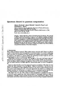
(b) Figure 1: Schematic representation of the model. (a) The system S consists of a register R of qubits plus ancillas A that can be reset during the computation. The system S is coupled to the environment, or bath, B. (b) The decoherence model. Each qubit qi is coupled to an individual bath Bi . When two qubits interact, they may interact with one common bath. The following assumptions have been shown to be necessary for fault-tolerance and thus we keep these assumptions in our analysis: • It is possible to operate gates on different qubits in parallel.

1 INTRODUCTION

3

• We have fresh ancilla qubits to our disposal. These ancilla qubits are prepared off-line in the exact computational state | 00 . . . 0i and they can be used in the circuit when necessary. They function as a heat-sink which removes entropy from the computation. . In Figure 1(a) three types of quantum systems are sketched that differ in function and in the amount of control that we can exert over them. First, there is R, for quantum Registers, that we can control and use for our computation. Secondly, there is A, for Ancillas, which are used for error-correction and faulttolerant gate construction during the computation. The systems R and A taken together are denoted as S for System of which single qubits are denoted by the letter q. Clean ancilla registers set to | 00 . . . 0i are added during the computation and can be removed after having interacted with (1) other parts of the system S by error-correcting procedures and (2) the bath B according to some fixed interaction Hamiltonian. We will assume that the third system, the bath B, which interacts with system and ancillas has a local structure, illustrated in Fig. 1(b). We will generalize this model in Section 3. Every qubit (q1 , q2 , q3 ...) of the system has its own bath (B1 , B2 , B3 ..). Only during the time when two qubits interact their baths (B1 and B2 in the figure) can interact. The idea behind this modelling is that the bath is localized in space, i.e. is associated with the place where the qubit is stored. But when qubits interact, they need to be brought together and so they may share a common bath. In the picture B1 + B2 at time t + t0 are suggested to be the same baths that qubits q1 and q2 interacted with at time t, but in general they may also be different baths. For example, when qubits q1 and q2 have to be moved in order to interact, they may see a partially new environment at time t + t0 . This distinction will not be important in our analysis. Most importantly, in this model, each bath can have an arbitrarily long memory; at no point in our derivation will we make a Markovian assumption. This implies that, for example, the bath B1 may contain information about qubit q1 at time t, then interact with bath B2 at time t + t0 and pass this information on to bath B2 etc. The interaction Hamiltonian of a single qubit qi of the system (R or A) with the bath is given by X HSB [qi ] = σk [qi ] ⊗ Ak . (1) k

with the Pauli-matrices σk acting on qubit qi and Ak is some Hermitian operator on the bath of the qubit qi which is not equal to the identity I. During a two qubit-gate both qubits may interact with both baths. For simplicity (see footnote [13]) we assume that the interaction is of the form HSB [qi , qj ] = HSB [qi ] + HSB [qj ],

(2)

where the bath part of each HSB [qi ] is an operator on the joint bath of qubits qi and qj . We do not care about the time-evolution of the baths except that it has to obey the “local bath assumption”, i.e. noninteracting qubits have noninteracting baths. The system (register and ancilla) evolution HRA (t) is time-dependent and represents the fault-tolerant quantum circuit that we want to implement. This evolution is built from a sequence of one and two qubit gates and, as was said before, t0 is the time it takes to perform any such gate.

1.2 Measure of Decoherence Strength Our results will depend on the strength of the coupling Hamiltonian HSB [qi ]. There is an additional freedom in determining HSB [qi ], namely we can always add a term αIS [qi ] ⊗ IB where α is an arbitrary real constant and I is the identity operator. This is possible since it merely shifts the spectrum (see footnote [14]). Let µi be the eigenvalues of HSB . With this freedom we see that min ||HSB [qi ] + αIS [qi ] ⊗ IB || = (µmax − µmin )/2 ≡ ∆SB [qi ], α

(3)

1 INTRODUCTION

4

the spectral width of the interaction Hamiltonian (divided by 2). Our analysis will apply to physical systems where one can bound ∀ qi ∈ S, ∆SB [qi ] ≤ λ0 . (4)

where λ0 is a small constant which will enter the threshold result, Theorem 1, together with t0 , the fundamental gate time. In what follows we will denote ∆SB [qi ] as ∆SB or ∆ assuming that the spectral width is the same for each qubit in S. We justify the use of this norm in the following way. Consider a single qubit coupled to a bath such that both bath and system Hamiltonians are zero but there exists nonzero coupling. To what extent will an arbitrary initial state of qubit and bath change under this interaction? We can consider the minimum fidelity of an initial state ψSB (0) with the evolved state at time t: Fmin (t) = min |hψ(t) |ψ(0)i|. ψ(0)

(5)

For small times t such that ∆SB t ≤ π/2 the minimum fidelity can be achieved by taking | ψ(0)i = √1 (| ψmax i + | ψmin i) where | ψmax/min i are the eigenvectors of HSB with largest and smallest eigenvalues. 2 Then we have Fmin (t) = cos(∆t) ≈ 1 − ∆2 t2 /2 + O((∆t)4 ). (6)

Note that this fidelity decay includes the effects on the bath. For this reason this fidelity decay overestimates the effects of decoherence, in other words F (ρS (t), ρS (0)) ≥ Fmin . One may compare this fidelity decay with that of other decoherence processes, for example the depolarizing channel E with depolarizing probability p. For such a channel we have F (| ψiS , E(| ψihψ |)S ) = q

1 − p2 [15]. Thus, loosely speaking, ∆t could be interpreted as an error amplitude whose square is an error probability. Thus, this brief analysis shows that for some initial states ψSB (0) the norm of the interaction Hamiltonian measures exactly how the state changes due to the interaction. Since our environment is non-Markovian we cannot exclude such bad initial states, in other words we cannot assume that the decoherence is just due to the interactive evolution of an initially unentangled bath and system.

1.3 Error Modelling Tools The following simple lemma will be used repeatedly in this paper: Lemma 1 Let a unitary transformation U = Un . . . U1 where Ui = Gi + Bi and the operator Gi and Bi are not necessarily unitary. Let U = B + G where we define B to be the sum of terms which contains at least k factors Bi . Let ||Bi || ≤ ǫ and thus ||Gi || ≤ 1 + ǫ. We have   n k ||B|| ≤ ǫ (1 + ǫ)n−k . (7) k If Gi is unitary, we have

  n k ||B|| ≤ ǫ . k

(8)

Proof: We can think about U as a binary tree of depth n such that the children of each node are labelled with Gi or Bi at depth i. We prune the tree in the following way; when a branch has k factors Bi in its path, we terminate this whole branch with the remaining U n . . . Um . The sum of these terminated branches n
is B. B can be bounded by observing that there are k terminated branches each of which have norm at most ||Bi ||k ||Gi ||n−k (since each branch is a sequence of Gi transformations interspersed with k Bi transformations followed by unitary transformations).

1 INTRODUCTION

5

It is easy to prove the following (see also Ref. [16]) Lemma 2 Consider a time-interval [t, t + t0 ] and a single qubit q ∈ S which does not interact with any other qubit in S at that time. The time-evolution for this qubit is given by some unitary evolution U [q] involving its bath B. Let U0 [q] = US [q] ⊗ UB be the free uncoupled evolution for this qubit. We can write U [q] = U0 [q] + E[q],

(9)

||E[q]|| ≤ t0 ||HSB [q]|| = t0 ∆SB [q] ≤ t0 λ0 .

(10)

where E[q] is a fault-operator with norm

Proof: We drop writing the dependence on qubit q for the proof. For the qubit evolution in the interval, using the Trotter expansion we can write tm tm U = lim Πnm=1 (UStm USB UB ). n→∞

(11)

where UKtm is the time-evolution for K = S, B or coupling SB during the time-interval tm of length t0 /n. t2 tm Now in this expansion we may write USB = I − iHSB t0 /n + O( n02 ) and omit these higher order terms. Let us call Gm = UStm UBtm and Bm = −i tn0 UStm HSB UBtm as in Lemma 1. We thus have ||Bm || ≤ tn0 ||HSB ||. Note that Gm is unitary and we have a binary tree of depth n → ∞ and can use Lemma 1 with k = 1. This gives ||E|| = ||B|| ≤ t0 ||HSB ||. (12)

A similar statement holds when we consider the evolution of two interacting qubits. We have that USB [qi , qj ] = U0 [qi , qj ] + E[qi , qj ],

(13)

where ||E[qi , qj ]|| ≤ 2t0 ∆SB [q] ≤ 2t0 λ0 .

1.4 Overall Perspective: good and bad fault-paths Since the bath may retain information about the time-evolution and error processes for arbitrary long times we cannot describe the decoherence process by sequences of superoperators on the system qubits. Instead, there is a single superoperator for the entire computation that is obtained by tracing over the bath at the end of the computation. Thus in our analysis we will consider the entire unitary evolution of system, bath and ancillas. At time t = 0 bath and ancilla and system are uncoupled and we may always purify the bath, i.e., find a pure state in a larger bath Hilbert space which, when the extra Hilbert space is traced out, yields the desired mixed state. We can then assume a pure initial product state for the combined system and bath, SB. The unitary evolution of the computation consists of a sequence and/or parallel application of the unitary gates U [qi , qj ](t+t0 , t) and U [qi ](t+t0 , t). Each such gate, say for two qubits, can be written as a sum of a error-free evolution U0 [qi , qj ](t + t0 , t) and a fault term E[qi , qj ]. Therefore the entire computation can be written as a sum over fault-paths, that it, a sum of sequences of unitary error-free operators interspersed with fault operators. This is very similar as in the fault-tolerance analysis for Markovian error models, where the superoperator during each gate-time t0 can be expanded in a error-free evolution and an erroneous evolution so that the entire superoperator for the circuit is a sum over fault-paths.

2 THRESHOLD RESULT

6

The main idea behind the threshold result for fault-tolerance is then as follows, see [4]. There are good fault-paths with so called sparse numbers of faults which keep being corrected during the computation and which lead to (approximately) correct answers of the computation. And there are bad fault-paths which contain too many faults to be corrected and imply a crash of the quantum computer. Now the goal of our fault-tolerance derivation which is completely analogous in structure as the one in [4] is to show the following: A Sparse fault-paths lead to sparse errors in the computation. This fact uses the formal distinction between faults that occur during the computation and the effects of these faults, the errors, that arise due the subsequent evolution which can spread the faults. The fact that sparse fault-paths give rise to sparse errors is due to fundamental properties of fault-tolerant error-correcting circuitry, namely that there exists error-correcting codes and procedures that do not spread faults too much. It is independent of the choice of decoherence model, and can be applied to any model where one can make an expansion into fault-paths. See Lemma 3. B Sparse errors give good final answers. This is a technical result whose derivation may differ slightly in one or the other decoherence model, but which is intuitively sound for all possible decoherence models. See Lemma 4. C The norm of the operator corresponding to all bad non-sparse fault-paths is “small”. This result depends crucially on the decoherence model that is chosen, in particular the spatial or temporal correlations that are allowed. Secondly, it depends on the strength of the errors, that is, only for small enough strength below some threshold value will the norm of the bad fault-path operator get small. See Section 2.2. A,B,C⇒ When the bad operator norm is small, the answer of the computation is close to what the good faultpath operator yields which is the correct answer according to item B. See Lemma 4 and Theorem 1. Another small comment about our model is the following: In the usual model for error-correction (see Ref. [6] in [17]), measurements are performed to determine the error-syndrome or the correct preparation of the ancilla states. Since we prefer to view the entire computation as a unitary process, we may replace these measurements by coherent quantum operations. In the error-correction with measurement procedures it is assumed that faults can occur in the measurement itself or in the quantum gate that is performed that depends on this measurement record, but the measurement record by itself is stable since it is classical. If we replace measuring by coherent action for technical reasons in this derivation, it is then fair to assume that the qubit that carries the measurement record is errorfree, in other words does no longer interact with a bath. This modelling basically allows the standard fault-tolerance results in item A expressed in Lemma 3, to carry over in the simplest way to our model.

2

Threshold result

2.1 Nomenclature Let the basic errorfree quantum circuit denoted by M0 consist of N locations [4]. Each location is given by a triple ({q}, G, t) where {q} denotes the qubits (one or two at most) involved in some gate G (G could be I) at time t in the quantum circuit. In the following, E[i] or U [i] will denote operators that involve location i, i.e. if q1 and q2 interact at location i we will write U0 [q1 , q2 ] = U0 [i] instead of enumerating the qubits. For fault-tolerance one constructs a family of circuits Mr by concatenation. That is, we fix a computation code C (see definition 15 in Ref. [4]), for example a CSS code, encoding one qubit into (say) m qubits

2 THRESHOLD RESULT

7

[18]. We obtain the circuit Mr by replacing each location in the circuit M0 by a block of encoded qubits to which we apply an error-correcting procedure followed by a fault-tolerant implementation of G, see Fig. 2. Repeated substitution will gives us a circuit Mr at concatenation level r.

E

Gfaulttol

G

E

M r−1

Mr

Figure 2: Every single or two-qubit gate G in the circuit Mr−1 gets replaced by an error-correcting procedure E followed by a fault-tolerant implementation of G, Gfaulttol (possibly involving ancillas).

Essential are the following definitions and a lemma taken from Ref. [4] which define sparseness of a set of locations and error-spread of a code: Definitions from Ref. [4]: • A set of qubits in Mr is called an s-block if they originate from 1 qubit in Mr−s . A s-working period in Mr is a time-interval which originates from one time-step in Mr−s . A s-rectangle in Mr is a set of locations that originate from one location in Mr−s . • Let B be a set of r-blocks in the circuit Mr . An (r, 1)-sparse set of qubits A in B is a set of qubits in which for every r-block in B, there is at most one (r − 1)-block such that the set A in this block is not (r − 1, 1)-sparse. A (0, 1)-sparse set of qubits in M0 is an empty set of qubits. • A set of locations in a r-rectangle is (r, 1)-sparse when there is at most 1 (r − 1)-rectangle such that the set is not (r − 1, 1)-sparse in that (r − 1)-rectangle. A fault-path in Mr is (r, 1)-sparse if in each r-rectangle, the set of faulty locations is (r, 1)-sparse. • A computation code C has spread s if one fault which occurs in a particular 1-rectangle affects at most s qubits in each 1-block at the end of that 1-rectangle, i.e. causes at most s errors in each 1-block. • Let AC be the number of locations in a 1-rectangle for a given code C. We state the basic lemma about properties of computation codes which was proved in Ref. [4] (with a correction). Lemma 3 (A: Lemma 8 in [4] with a correction) Let C be a computation code that can correct 2 errors and has spread s = 1. Consider a computation Mr subjected to a (r, 1)-sparse fault-path. At the end of each r-working period the set of errors is (r, 1)-sparse. Thus for simplicity we will be using a quantum computation code that encodes one qubit and can correct two errors and has spread s = 1. We denote the entire unitary evolution of Mr including the bath as Qr . We may write Qr = QrG + QrB where QrG is a sum over good (r, 1)-sparse fault-path operators and QrB contains

2 THRESHOLD RESULT

8

the bad non-sparse terms. A fault-path operator ESB that is (r, 1)-sparse is a sequence of free evolutions U0 [i] for all locations except that in every r-rectangle there is a (r, 1)-sparse set of locations where a fault operator E[i] occurs. Definition 1 (Operators in the Interaction Picture) Let U0 (t2 , t1 ) = US (t2 , t1 ) ⊗ UB (t2 , t1 ) be the free uncoupled evolution of system and bath in the time-interval [t1 , t2 ]. We define a fault-operator E(t2 , t1 ) in the interaction picture as E(t2 , t1 ) = U0 (t2 , t1 )E U0† (t2 , t1 ). (14) The interpretation is that E(t2 , t1 ) is the spread of a fault E that occurs at t1 due to the subsequent free evolution. Then it is simple to see the following: Proposition 1 (Error Spread in the Interaction Picture) Consider a quantum circuit M . Let U0 (tF , tI ) be the uncoupled evolution for M . Faults occur at a set of ‘time-resolved’ locations T = ((i1 , t1 ), (i2 , t2 ), . . . , (ik , tk )) where i1 , . . . , ik is the set of distinct locations of the faults and t1 , . . . , tk label the specific times that the faults occur at the locations. Let ESB (T ) be a particular fault-path operator in which at every faulty location (i, t) ∈ T we replace U0 [i] by a fault-operator E[i]. We have ESB (T )U0† (tF , tI ) = E[ik ](tF , tk ) . . . E[i1 ](tF , t1 ).

(15)

We note that the system part of ESB U0† is I everywhere except for the qubits that are in the causal cone of the faulty locations, i.e. the qubits to which the errors potentially have spread. Proof: This can be shown by inserting I = U0† (tF , ti )U0 (tF , ti ) in the appropriate places and then using the definition of fault operators in the interaction picture. Now we include error-correction and differentiate between the ancilla systems A used for error-correction which may contain noise and the registers R in which the errors remain sparse. Note that all these ancillas are in principle discarded after being used, but we may as well leave them around. Let K|C be the restriction of the operator K to vectors in the code-space of C, i.e. K|C = K PC where PC is the projector on the codespace. Let us consider a fault-path operator ESB representing a single fault E at time t on some block that is subsequently corrected by an errorfree error-correcting procedure. Let | INi be the initial state of the computer, bath and ancillas and U0 (tF , tI ) be the perfect evolution. We have ESB | INi = ESB U0† U0 | INi = ESB U0† | ψC (tF )i.

(16)

where | ψC (tF )i is the final perfect state of the computer, prior to decoding and therefore in the code-space. ESB is the sequence U0 (tF , t)E U0 (t, t0 ) where U0 (tF , t) includes the error correction operation. In other words, in the interaction picture, we can write ESB | INi = E(tF , t)| ψC (tF )i,

(17)

The error-correcting conditions (see [15], par. 10.3) imply that when acting on the code space and an ancilla state set to | 00 . . . 0i the operator E(tF , t) will be E(tF , t) = I|C ⊗ (Junk)AB where Junk is some arbitrary operator on the ancilla (that receives the error syndrome in the error-correcting procedure) and bath. In Eq.

2 THRESHOLD RESULT

9

(17) the final errorfree state has all ancillas set to | 00 . . . 0i and the system state is in the code-space and thus the error acts as I on the system. Similarly, let ESB contain two faults at times t1 < t2 that have not spread (say) and are then corrected by a perfect error-correcting procedure. We have ESB | INi = E2 (tF , t2 )E1 (tF , t1 )| ψC (tF )i.

(18)

Let us assume, for example, that E1 occurs prior to error-correction and E2 occurs during error-correction. Then due to the error correction E1 (tF , t1 ) acts as I on the code space when the ancilla used for errorcorrection is set to | 00 . . . 0i and acts as Junk on this ancilla and the bath. The error E2 will not be corrected and may still be present (but will not have spread to more qubits in the block due to the spread properties of the code that is used) after error- correction. Thus in total we can write for this process that E1 (tF , t1 ) acts as I on the code space, whereas E2 (tF , t2 ) is an operator that acts on the code space as at most one error per block. Alternatively, both faults could occur prior to error-correcting so they can both be corrected by our code. This implies that both E1 (tF , t1 ) and E2 (tF , t2 ) act as I on the code-space. Note that after the first fault the ancilla will be partially filled (i.e. not be | 00 . . . 0i) but since the code can correct two errors there is still space to put the second error syndrome in. However a third operator E3 (tF , t3 ) would no longer act as I on the code-space since the code cannot correct three errors. In other words, with these examples we can see how Lemma 3 can be translated in terms of the sparseness of the errors in the interaction picture, i.e. the sparseness of places where they act as non-identity on the final encoded state of the register qubits. In the next lemma we need to consider the effect of such sparse fault-path operators ESB on the final state of the computer. This is the state of the computer obtained after fault-tolerant decoding which is as follows. The fault-tolerant decoding procedure for a single level of encoding takes a codeword | ci and ‘copies’ (by doing CNOT gates) the codeword m times. Then on each ‘copy’ we determine what state it encodes and then we take the majority of the m answers. This procedure is done recursively when more levels of encoding are used. In the fault-tolerant decoding procedure faults can occur on the codewords, i.e. as incoming faults, during the copying procedures and during the determination of what is encoded by the codeword. The last procedure will usually be a conversion from a quantum state to a classical bit string since this will be the most efficient. This implies that the step of taking the recursive majority of these bits is basically errorfree since it only involves classical data. In the next Lemma we model this by coherent quantum operations that output superpositions of decoded bit strings followed by an error-free measurement that takes the recursive majority of these bits. Lemma 4 (B: Sparse faults give almost correct answers) Let Qr = QrG + QrB the unitary evolution of Mr and let ||QrB || ≤ ǫ < 1/2. Let P0 (i) be the output probability distribution under measurement of some set of qubits of the error-free original computation M0 . Let P(i) be the simulated output distribution of the encoded computation Mr with evolution Qr . We have √ (19) ||P0 − P||1 ≤ 2ǫ + 16ǫ.

Proof: The initial state of the computer is | INiRAB = | 00 . . . 0iRA ⊗ | INB i for some arbitrary state | INB i. Let U0r be the error-free evolution of Mr including the final decoding operation. Thus let U0r | INiRAB = | OUT0 iR ⊗ | RESTiAB . Let Qr | INiRAB = | OUTiRAB and QrB/G | INiRAB = | OUTB/G iRAB . We will drop the label RAB from now on. The norm of | OUTG i will be denoted as ||OUTG ||. We have 1 = ||Qr | INi|| ≤ ||QrG | INi|| + ||QrB | INi||,

(20)

2 THRESHOLD RESULT

10

so that ||OUTG || ≥ 1 − ||QrB | INi|| ≥ 1 − ǫ. On the other hand ||QrGP || = ||Qr − QrB || ≤ 1 + ǫ. Let G be the set of (r, 1)-sparse fault-paths. We have QrG = T ∈G ESB (T ) where ESB (T ) is the fault-path operator of a (r, 1)-sparse fault-path labelled by location and time index set T . We can write X | OUTG i = ESB (T )U0r † | OUT0 iR ⊗ | RESTiAB . (21) T ∈G

By the arguments above and the fundamental Lemma 3 we know that ESB (T )U0† is I everywhere except on a (r, 1)-sparse set of qubits. Let w be the number of output qubits of M0 . The ideal state | OUT0 iR has the property that all qubits in an r-block have the same value in the computational basis, i.e. X r r | OUT0 iR = (22) αi1 ...iw | i1 i⊗m . . . | iw i⊗m , i1 ,...,iw

where m is the number of qubits in a 1-block. The final step of the computation is a measurement of all output qubits that takes the recursive majority on the block to get the final output P string i of length w tot with probability P (i). We model this measurement using POVM elements Ek , – k Ek = I. Since not all these w output bits may be relevant output bits of M0 , we may use the fact that trace-distance is non-increasing over tracing [15] so that tot ||P0 − P||1 ≤ ||Ptot 0 − P ||1 ,

(23)

where Ptot (k) = TrEk | OUTihOUT |RAB and Ptot 0 (k) = TrEk | OUT0 ihOUT0 |R . Let us also define Ptot , the distribution of outcomes if the state of the computer would be the normalized state | OUTN Gi ≡ G | OUTG i/||OUTG ||. The triangle inequality and the properties of the trace-norm imply that tot tot tot ||Ptot − Ptot − Ptot 0 ||1 ≤ ||P G ||1 + ||PG − P0 ||1 ≤

N tot tot || | OUTihOUT | − | OUTN G ihOUTG | ||1 + ||PG − P0 ||1 .

(24)

Here the first term can be bounded, using the relation of the trace norm to the fidelity F (ψ, φ) = |hψ |φi| [15], as q
2 N 1 − F OUT, OUTN ≤ || | OUTihOUT | − | OUTN ihOUT | || ≤ 1 G G G p p 1 − ||OUTG ||2 ≤ 2ǫ − ǫ2 . (25)

Now consider the second tracenorm on the r.h.s. of Eq. (24). We note that all states that are linear combinar r tions of (r, 1)-sparse error sets applied to the state | k1 i⊗m . . . | kw i⊗m will give rise to the measurement outcome k since we are taking majorities. We can model Ek = Pk where Pk is the projector onto the space of computational basis states that give rise to the majority output string k. Thus we have X r r (26) ESB (T )U0r † | k1 i⊗m . . . | kw i⊗m ⊗ | RESTiAB . Pk | OUTG i = αk1 ...kw T ∈G

which can be written as αk1 ...kw QrG | ψk i for some normalized state | ψk iRAB . This implies that the second term in Eq. (24) can be bounded as r 2 X tot tot 2 ||QG | ψk i|| ||PG − P0 ||1 = − 1 ≤ |αk1 ...kw | 2 ||OUTG || k X ||QrG | ψk i||2 4ǫ 2 ≤ |αk1 ...kw | max − 1 , (27) 2 k ||OUTG || (1 − ǫ)2 k

using the bounding inequalities of ||QrG || and ||OUTG ||. All bounds put together, using ǫ < 1/2, give the result, Eq. (4).

2 THRESHOLD RESULT

11

2.2 Step C: non-sparse fault-paths have small norm Consider the evolution Qr which can be viewed as a sequence of unitary evolutions, one for each rrectangle, since qubits in different rectangles do not interact. The number of locations in M0 is N . The computation Qr is bad when at least one r-rectangle is bad, or using Lemma 1 r r N −1 ||QrB || ≤ N ||RB || ||RG || ,

(28)

r and Rr are the good and bad parts of the unitary evolution Rr for some r-rectangle. The unitarity where RB G r r || ≤ 1 + ||Rr ||. In each rectangle we can view the entire evolution of R implies that we can bound ||RG B as a sequence of unitary evolutions, one for each (r − 1)-rectangle. Note that we are again using the fact that non-interacting qubits have non-interacting baths. A r-rectangle is bad when there are at least two (r − 1)-rectangles which contain sets of faulty locations which are not (r − 1, 1) sparse. This implies, using Lemma 1 again, that   AC r−1 AC −2 r−1 2 r || , (29) || ≤ ||RB || ||RG ||RB 2

r−1 r−1 1 is a unitary operation and thus ||R1 || = 1. ||. When r = 1, RG || ≤ 1 + ||RB where we can use that ||RG G This recurrence in r is identical to the one in Lemma 11 in Ref. [4] and thus the solution and results are the same if we replace η in Ref. [4] by λ0 t0 . Thus the critical error threshold value is 1 . (30) (λ0 t0 )c = eAC (AC − 1)

Here we can observe a difference with the simplest error model with error probability p for which the critical value is pc = A1C [4]. The dimensionless quantity λ0 t0 plays the role of an amplitude, see Sec. 5, (2) which implies that this threshold value may be more stringent than in the simple probabilistic error model (see also the critique by Alicki [19] on our results). However, we believe that this analysis is too course to really give information about the value of the threshold. The fact is that in practice, baths do not have infinite memory times since they are coupled to many other degrees of freedom. Representing the coupling between bath and system as a pure coherent evolution was needed in this analysis to deal with the non-Markovian dynamics; however, we do not expect this formal procedure to give rise to an optimal error threshold. The idea of the remaining derivation given in Ref. [4] is to show that when λ0 t0 < (λ0 t0 )c for large enough concatenation level r, ||QrB || ≤ ǫ for arbitrary small ǫ. Lemma 4 then tells how much our quantum computation errs from the error-free computation. Summarizing we get the following, as in Ref. [4]: Theorem 1 (Threshold Theorem for Local Non-Markovian Noise) Let N be the number of locations of an errorfree quantum computation M that outputs samples from a probability distribution P. There exists a quantum circuit M ′ subjected to noise according to the Hamiltonian HSB and bath Hamiltonian HB that obeys the “noninteracting qubits have noninteracting baths” assumption which outputs the probability distribution P′ such that ||P′ − P||1 ≤ ǫ, (31) when ∆SB t0
t0 Non-Markovian with unlimited memory time

Single Location Baths X

Cluster Location Baths at r = 1 X

Arbitrary Baths ?

X

X

?

X

X

?

Table 1: A X indicates that a fault-tolerance result exists whereas a question mark ? indicates that it is not known to exist so far (neither has it been disproved). The results for non-Markovian baths assume a 1-systemlocal interaction Hamiltonian that can be bounded in norm. They also assume that we can do two-qubit gates between any two qubits in the circuit (that is, we do not take physical locality constraints into account). The assumptions on the structure of the system-bath interaction and the bath Hamiltonian are given by the three columns. Single Location Baths implies that the interaction and the baths are constrained so that for each elementary time-interval (clock-cycle) [t, t + t0 ] the following condition is obeyed: qubits that do not interact can only interact with baths which do not interact, see Fig. 1(b). Note that the particular baths with which the qubits interact may change over time. Cluster Location Baths is the extension of this model covered in Section 3 where a cluster of qubits can share the same bath, see Fig. 3. In the last column there is no constraint on the bath. an error with probability p and undergoes no error with probability 1 − p. This is a specific example of a Markovian model in which in every location has its own separate environment, i.e we have “Single Location Baths”, see the upper left entry in the Table 1. Generalizations of this model exist [4, 3]; in these models a superoperator S(ρ) = S0 (ρ) + E(ρ) where S0 corresponds to the error-free evolution and E to the erroneous part, is associated with each location. Again this corresponds to the upper left entry in the table. This model has been generalized to allow for more general correlations in space and time in the following manner. In Ref. [4] fault-tolerance was derived in a model where it is assumed that the probability for a fault-path with k faults is bounded by Cpk (1 − p)N −k where N is the total number of locations in the circuit (note the difference with Eq. (43) in Appendix A). Similarly, in Ref. [3] fault-tolerance was derived under the assumption that a fault-path with at least k faults has probability bounded by Cpk for some constant C. Let us call these conditions the exponential decay conditions. Note in the Table that it is not known whether one can derive fault-tolerance for a entirely Markovian model but with extended spatial correlations between the baths, i.e. for every clock-cycle we have a superoperator that acts on all qubits of the system; the point is that it is not clear whether such a superoperator would obey some sort of exponential decay conditions.

5

Measures of Coupling Strength and Decoherence

In our analysis the role of error amplitude is played by the dimensionless number λ0 t0 which captures the relative strength of the interaction Hamiltonian as compared to the system Hamiltonian. It is this quantity, λ0 t0 , that should be O(10−4 ) as was determined for some codes. In a purely Markovian analysis we typically replace λ0 by an inverse T2 or T1 time and this may give a more optimistic idea of the regime of fault-tolerance. Let us consider a few examples of decoherence mechanisms and see how sensible it is to use ∆SB as a bound for decoherence. A good example of a non-Markovian decoherence mechanism is a small finite dimensional environment localized in space, for example a set of spins nearby the system of interest.

5 MEASURES OF COUPLING STRENGTH AND DECOHERENCE

15

An example is the decoherence in NMR due to interactions with nuclear spins in the same molecule. In NMR the nuclear exchange coupling between spins a and b is given Hint = Jab I~a · I~b .

(34)

If the J-coupling is treated as a source of decoherence as compared to the Zeeman-splitting ω0 for an individual spin, then J/ω0 can be ∼ 10−6 (see footnote [27]). For some physical systems a source of decoherence is a bath of spins, each of which couples to a single qubit. An example is the electron spin qubit in a single quantum dot which couples via the hyperfine coupling to a large set of nuclear spins in the semiconductor [28]. The interaction Hamiltonian is as follows Hint =

N X i=1

~ a(i) ~σ · I[i],

(35)

where a(i) = Av0 |ψs (i)|2 and A is the hyperfine coupling constant, v0 the volume of the P crystal cell, and |ψs (i)|2 is the probability of the electron to be at the position of nuclear spin i. If we bound i |ψs (i)|2 ≤ 1 we have that ||Hint || ≤ CAv0 where C is a small constant (of order 1). This may give a somewhat weak upper bound on the decoherence, since we are basically adding the effects of each nuclear spin separately. A third type of decoherence mechanism exists which is essentially troublesome in our analysis. This is the example of a single qubit, or spin, coupled to a bosonic bath. The interaction Hamiltonian is that of the spin-boson model [29] N X (ci ai + c∗i a†i ), (36) Hint = σz ⊗ i=1

where i labels the ith bosonic mode characterized by frequency ωi . The ith bosonic mode has Hamiltonian N go to infinity. In that HBi = ωi (a†i ai + 21 ). In order to represent a continuous bath spectrum, one lets P 2 limit the coupling constants ci are determined by the spectral density J(ω) = i |ci | δ(ω − ωi ). The spectral density can have various forms, matching the phenomenology of the particular physical system, an example is the Ohmic form in which J(ω) = αωe−ω/ωc where α is a weak coupling constant that has physical relevance and ωc is a cutoff frequency that is also determined by the physics. It is clear that ||Hint || has no physical meaning since it is infinite, the reason being that there are infinitely excited bath states with infinitely high energy. We can determine an energy-dependent upper bound on this norm; using properties of the norm, we can estimate X X ||Hint | ψiSB || = || ci ai + c∗i a†i )| ψiSB || ≤ |ci |(||ai | ψiSB || + ||a†i | ψiSB ||) i

i

≤ Using the Schwartz inequality we get s ||Hint | ψiSB || ≤ 2

X |ci |2 i

ωi

X |ci | p 4hψ |HBi | ψiSB . √ ωi

(37)

i

s

hψ |HB | ψiSB = 2

hHB iψSB

Z

∞ 0

dω

J(ω) . ω

(38)

P for some state of system and bath | ψiSB where the bath Hamiltonian HB = i HBi . The idea is that for the physically relevant states of the bath hHB iψ is bounded. The problem remains that this bound will in general be too poor to be physically relevant, since this energy bound may be quite large. Also, for ohmic coupling R∞ (for example) we have the integral 0 dω J(ω) ω = α ωc , i.e. linear in ωc . The cutoff ωc may be quite large and it is more typical to see decoherence rates depend on log ωc as in the non-Markovian analysis of Ref. [30] for example.

6 CONCLUSION

16

5.1 Cooling assumption Some progress can be made in finding good bounds for ||Hint || in the case of a bosonic environment if additional assumptions about its state can be made. What is troublesome about the potential nonequilibrium state of the bath is that expectation values such as Tr ai aj | ψihψ |SB and Tr a2i | ψihψ |SB may not be zero since the bath state may not be diagonal in the energy or boson number basis. On the other hand, interaction with other environments, for example by means of cooling, will dephase the state of the bath (due to energy exchange) and drive it to a state that is diagonal in the energy eigenbasis. Under that assumption only the terms Tr a†i ai | ψihψ |SB and Tr ai a†i | ψihψ |SB are nonzero. In that scenario, Eq. (37) simplifies to sX |ci |2 hψ |a†i ai + I/2)| ψiSB . (39) ||Hint | ψiSB || ≈ i

Still, ||Hint | ψiSB || can be very large if some modes of the environment are highly excited, ni = a†i ai ≫ 1. However, in a realistic setting, this will be prevented by cooling the bath, i.e. by constantly removing energy from it. Without making a Markov approximation, we can thus assume that the occupation numbers ni of the bath are upper-bounded by those of a thermal distribution with an effective maximal temperature Teff . This gives sZ ∞ J(ω) coth(βeff ω/2)/2, (40) ||Hint | ψiSB || / 0

where βeff =

1 kB Teff .

We can evaluate Eq. (40) for the Ohmic case using Mathematica r s 2Ψ′ ( βeff1ωc ) α 2 ||Hint | ψiSB || / , −ωc + 2 2 βeff

(41)

′

(x) where Γ(x) is the Gamma funcwhere Ψ′ (x) is the first derivative of the digamma function Ψ(x) = ΓΓ(x) 1 tion. For βeff ωc ≪ 1 we do a series expansion and obtain r s    2 1 α π 1 2 +O . (42) ||Hint | ψiSB || / ωc + 2 2 3 βeff ωc βeff

Unlike Eq. (38), this bound does not involve extensive quantities, such as the total energy hHB iψSB of the bath. However, Eq. (42) still involves the high-frequency cut-off ωc because of the zero-point fluctuations of the bath.

6

Conclusion

Some important open questions remain in the area of fault-tolerant quantum computation. Most importantly, is there a threshold result for non-Markovian error models with system-local Hamiltonians and no further assumptions on the bath? Is this a technical problem, i.e. how can one efficiently estimate QrB , or are there specific malicious system-bath Hamiltonians that have such effect that the norm of the bad faults does not become smaller when increasing r? The next question is whether a better analysis is possible for the spin-boson model, which is a highly relevant decoherence model. One would like to evaluate the effect of HSB in the sector of physical states, but the characterization of these physical states is unclear due to the non-Markovian dynamics. For real systems one is probably interested in a finite memory time τ > t0 which may be simpler to solve. For example, one can derive the superoperator for a single spin qubit coupled to a bosonic bath in the Born approximation [30], however a derivation involving more than one system qubit may be too hard to do analytically.

A BOUNDS ON FAULT-PATH NORMS

17

6.1 Acknowledgements We would like to thank David DiVincenzo and Dorit Aharonov for helpful discussions and Andrew Steane for comments and suggestions. This work was supported in part by the NSA and the ARDA through ARO contract No. DAAD19-01-C-0056.

A

Bounds on Fault-Path Norms

Lemma 6 (Fault-Path Norms) Consider the entire unitary evolution Qr of a quantum computation on SB. Let ∀q ∈ S, ∆SB [q] ≤ λ0 . We expand Qr as a sum over fault-paths which are characterized by a set of faulty locations I. A fault-path operator with k faults has norm bounded by ||E(Ik )|| ≤ (2λ0 t0 )k .

(43)

Proof: We do a Trotter-expansion of Qr and obtain a tree with an infinite number of branches each of which corresponds to a certain time-resolved fault-path. Every time a fault occurs at some time tm and location im we append unitary evolutions for the remaining time of the location, since we do not care that more faults occur in that time-interval, the location has failed anyway. These time-resolved fault-path are characterized by an index set T = ((i1 , t1 ), (i2 , t2 ), . . . , (ik , tk )) where i1 , . . . , ik is the set of locations of the faults and t1 , . . . , tk label the specific times that the faults occur at the locations. Every such time-resolved faultoperator with k faults has norm bounded   2tλ0 k . (44) ||E(Tk )|| ≤ n Now we need to group these time-resolved fault-paths corresponding to faults at sets of locations. For fixed n faults can occur in time-intervals of length t/n and thus during a time t0 t0tn time-resolved faults can occur. This implies that X ||E(Ik )|| ≤ || ||E(Tk )|| ≤ (2λ0 t0 )k . (45) Tk →Ik

References [1] P. W. Shor. Fault-tolerant quantum computation. In Proceedings of 37th FOCS, pages 56–65, 1996. [2] D. Aharonov and M. Ben-Or. Fault tolerant quantum computation with constant error. In Proceedings of 29th STOC, pages 176–188, 1997, http://arxiv.org/abs/quant-ph/9611025. [3] E. Knill, R. Laflamme, and W. Zurek. Resilient quantum computation: Error models and thresholds. Proc. R. Soc. Lond. A, 454:365–384, 1997, http://arxiv.org/abs/quant-ph/9702058. [4] D. Aharonov and M. Ben-Or. Fault-tolerant Quantum Computation with Constant Error Rate. To appear in the SIAM Journal of Computation, http://arxiv.org/abs/quant-ph/9906129.

REFERENCES

18

[5] D. Gottesman. A theory of fault-tolerant quantum computation. Phys. Rev. A, 57:127, 1998, http://arxiv.org/abs/quant-ph/9702029. [6] J. Preskill. Fault-tolerant quantum computation. In Lo et al. [17], pages 213–269. [7] E. Knill, R. Laflamme, and W. Zurek. Resilient quantum computation. Science, 279:342–345, 1998. [8] A.M. Steane. Overhead and noise threshold of fault-tolerant quantum error correction. Phys. Rev. A, 68:042322, 2003, http://arxiv.org/abs/quant-ph/0207119. [9] W. D¨ur and H.-J. Briegel. Entanglement purification for quantum computation. Phys. Rev. Lett., 90:067901, 2003, http://arxiv.org/abs/quant-ph/0210069. [10] E. Knill. Scalable quantum computation in the presence of large detected-error rates. 2003, http://arxiv.org/abs/quant-ph/0312190. [11] A. Kitaev. Fault-tolerant quantum computation by anyons. http://arxiv.org/abs/quant-ph/9707021.

Annals Phys. 303:2, 2003;

[12] R. Alicki, M. Horodecki, P. Horodecki, and R. Horodecki. Dynamical description of quantum computing: generic nonlocality of quantum noise. Phys. Rev. A, 65:062101, 2002. [13] We could alternatively use an interaction that involves a ‘three body’ term such as σk [qi ] ⊗ σl [qj ] ⊗ Akl , but this will not make much difference in the analysis. [14] The freedom is really stronger than this. We could add a term IS [q] ⊗ OB for arbitrary bath operator OB acting on the bath of qubit q since our analysis (basically Lemma 2) will not depend on the bath dynamics. It is not clear that this extra freedom makes a big difference in the analysis. For example, it can be proven that it does not solve the problems that we face with the norm of the interaction Hamiltonian for the spin-boson bath, see Section 5. [15] M. A. Nielsen and I. L. Chuang. Quantum computation and quantum information. Cambridge University Press, Cambridge, U.K., 2000. [16] E. Knill, R. Laflamme, and L. Viola. Theory of quantum error correction for general noise. Phys. Rev. Lett., 84:2525–2528, 2000, http://arxiv.org/abs/quant-ph/9908066. [17] H.-K. Lo, S. Popescu, and T.P. Spiller, editors. Introduction to Quantum Computation. World Scientific, Singapore, 1998. [18] Codes encoding more that one qubit could also be used, but they will complicate the analysis. [19] R. Alicki. Comments on ”Fault-Tolerant Quantum Computation for Local Non-Markovian Noise”. 2004, http://arxiv.org/abs/quant-ph/0402139. [20] We could generalize this to c-systemlocal Hamiltonians without much ado. [21] J. Preskill. Fault-tolerant quantum computation. pages 213–269. World Scientific, Singapore, 1998. [22] E. Knill. Scalable quantum computation in the presence of large detected-error rates. 2003, http://arxiv.org/abs/quant-ph/0312190.

REFERENCES

19

[23] D.J. Wineland, M. Barrett, J. Britton, J. Chiaverini, B. DeMarco, W.M. Itano, B. Jelenkovic, C. Langer, D. Leibfried, V. Meyer, T. Rosenband, and T. Sch¨atz. Quantum information processing with trapped ions. To appear in Proceedings of the Discussion Meeting on Practical Realisations of QIP, held at the Royal Society, 2002, http://arxiv.org/abs/quant-ph/0212079. [24] K.M. Svore, B.M. Terhal, and D.P. DiVincenzo, Local Fault-Tolerant Quantum Computation, http://arxiv.org/abs/quant-ph/0410047. [25] D. Gottesman. Fault-tolerant quantum computation with local gates. Jour. of Modern Optics, 47:333–345, 2000, http://arxiv.org/abs/quant-ph/9903099. [26] A. Steane. Quantum computer architecture for fast entropy exchange. Quantum Information and Computation, 2(4):297–306, 2002, http://arxiv.org/abs/quant-ph/0203047. [27] Of course methods also exist for turning off unwanted J-couplings by refocusing. [28] A. Khaetskii, D. Loss, and L. Glazman. Electron spin decoherence in quantum dots due to interaction with nuclei. Phys. Rev. B, 67:195329, 2003, http://arxiv.org/abs/cond-mat/0211678. [29] U. Weiss. Quantum Dissipative Systems. World Scientific, Singapore, 2000. [30] D. Loss and D.P. DiVincenzo. Exact Born approximation for the spin-boson model. http://arxiv.org/abs/cond-mat/0304118.