Fault-Tolerant Quantum Computation With Constant Error Rate

FAULT-TOLERANT QUANTUM COMPUTATION WITH CONSTANT ERROR RATE

∗

DORIT AHARONOV† AND MICHAEL BEN-OR‡

arXiv:quant-ph/9906129v1 30 Jun 1999

Key Words: Quantum computation, Noise and Decoherence, Density matrices, Concatenated quantum error correcting codes, Polynomial codes, Universal quantum gates

Abstract. Shor has showed how to perform fault tolerant quantum computation when the probability for an error in a qubit or a gate, η, decays with the size of the computation polylogarithmically, an assumption which is physically unreasonable. This paper improves this result and shows that quantum computation can be made robust against errors and inaccuracies, when the error rate, η, is smaller than a constant threshold, ηc . The cost is polylogarithmic in space and time. The result holds for a very general noise model, which includes probabilistic errors, decoherence, amplitude damping, depolarization, and systematic inaccuracies in the gates. Moreover, we allow exponentially decaying correlations between the errors both in space and in time. Fault tolerant computation can be performed with any universal set of gates. The result also holds for quantum particles with p > 2 states, namely qupits, and is also generalized to one dimensional quantum computers with only nearest neighbor interactions. No measurements, or classical operations, are required during the quantum computation. We use Calderbank-Shor Steane (CSS) quantum error correcting codes, generalized to qupits, and introduce a new class of CSS codes over Fp , called polynomial codes. It is shown how to apply a universal set of gates fault tolerantly on states encoded by general CSS codes, based on modifications of Shor’s procedures, and on states encoded by polynomial codes, where the procedures for polynomial codes have a simple and systematic structure based on the algebraic properties of the code. Geometrical and group theoretical arguments are used to prove the universality of the two sets of gates. Our key theorem asserts that applying computation on encoded states recursively achieves fault tolerance against constant error rate. The generalization to general noise models is done using the framework of quantum circuits with density matrices. Finally, we calculate the threshold to be ηc ≃ 10−6 , in the best case. The paper contains new and significantly simpler proofs for most of the known results which we use. For example, we give a simple proof that it suffices to correct bit and phase flips, we significantly simplify Calderbank and Shor’s original proof of the correctness of CSS codes. We also give a simple proof of the fact that two-qubit gates are universal. The paper thus provides a self contained and complete proof for universal fault tolerant quantum computation.

1. Outline. Quantum computation has recently gained a lot of attention, due to oracle results[65, 10, 11] and quantum algorithms[25, 65, 36], in particular Shor’s factorization algorithm [62]. These results indicate a possibility that quantum computers are exponentially more powerful than classical computers. It is yet unclear whether and how quantum computers will be physically realizable[19, 22, 30, 37, 50, 51, 55, 59, 69] but as any physical system, they in principle will be subjected to noise, such as decoherence [76, 71], and inaccuracies. Thus, the question of correcting noise cannot be separated from the complexity questions. Without error corrections, the effect of noise will accumulate and ruin the entire computation[72, 17, 54, 52, 7], and hence the computation must be protected. For classical circuits, von Neumann has shown already in 1956 ∗A

preliminary version of this paper, under the name “Fault-Tolerant Quantum Computation With Constant Error”, was

published in Proceedings of the 29th Annual ACM Symposium on Theory of Computing (STOC) 1997 † School of Mathematics, Institute for Advanced Studies, Princeton, New Jersey ‡ Department of Computer Science, The Hebrew University, Jerusalem, Israel 1

that the computation can be made robust to noise[53]. However, the similar question for quantum systems is much more complicated. Even the simpler question of protecting quantum information is harder than the classical analogue because one must also protect the quantum correlations between the quantum bits (qubits). It was argued by scientists that due to the continuity of quantum states, and to the fact that quantum states cannot be cloned[74], it will be impossible to protect quantum information from noise[72, 47]. Despite these pessimistic beliefs, Shor discovered a scheme to reduce the effect of decoherence[63]. Immediately after that, Calderbank and Shor[13] and Steane[68] showed that good quantum error correcting codes exist, a result which was followed by many explicit examples of quantum codes (e.g.[46, 68]). A theory for quantum error correcting codes was developed[43], and a group theoretical framework for almost all codes was found [14, 15, 31]. The existence of quantum error correcting codes, however, does not imply the existence of noise resistant quantum computation, since due to computation the faults propagate. One must be able to compute without allowing the errors to propagate too much, while error corrections should be made in the presence of noise. Recently Shor[64] showed how to use quantum codes in order to perform fault tolerant quantum computation in the presence of probabilistic errors, when the error rate, or the fault probability each time step, per qubit or gate, is polylogarithmically small. This assumption is physically unrealistic. In this paper we improve this result and show how to perform fault tolerant quantum computation in the presence of constant error rate, as long as the error rate η, is smaller than some constant threshold, η0 . The result holds for a very general noise model, which includes, besides probabilistic errors, also decoherence, amplitude and phase damping, depolarization, and systematic inaccuracies in the gates. Fault tolerance can be achieved using any universal set of gates. The result also holds when working with quantum particles of more than two states, instead of qubits. Our scheme can be generalized to work also in the case in which the quantum computer is a one dimensional array of qubits or qupits, with only nearest neighbor interactions. No measurements, or classical operations, are required during the quantum computation. The cost is polylogarithmic in the depth and size of the quantum circuit. The main assumption on the noise is that of locality, i.e. the noise process in different gates and qubits is independent in time and space. This assumption can be slightly relaxed, by allowing exponentially decaying correlations in both space and time. Such assumptions are made also in the classical scenario, and are likely to hold in physical realizations of quantum computers. Thus, this paper settles the question of quantum computation in the presence of local noise. Let us first describe the computational model with which we work. The standard model[23, 24, 75] of quantum circuits with unitary gates, allows only unitary operations on qubits. However, noisy quantum systems are not isolated from other quantum systems, usually referred to as the environment. Their interactions with the environment are unitary, but when restricting the system to the quantum computer alone the operation on the system is no longer unitary, and the state of the quantum circuit is no longer a vector in the Hilbert space. It is possible to stay in the unitary model, keeping track of the state of the environment. However, this environment is not part of the computer, and it is assumed that we have no control or information on its state. We find it more elegant to follow the framework of the physicists, and to work within the model of quantum circuits with mixed states defined by Aharonov, Kitaev and Nisan[4]. In this model, the state of the set of qubits is always defined: It is a probability distribution over pure states, i.e. a 2

mixed state, or a density matrix, and not merely a pure state as in the standard model. The quantum gates in this model are not necessarily unitary: any physically allowed operator on qubits is a quantum gate. In general, it is easiest to think of a general physical operator as a unitary operation on the system of qubits and any number of extra qubits, followed by an operator which discards the extra qubits. In particular, one can describe in this model an operation which adds a blank qubit to the system, or discards a qubit. The model of quantum circuits with mixed states is equivalent in computational power to the standard model of quantum circuits[4], but is more appropriate to work with when dealing with errors. The noise process can be described naturally in this model as follows. Since noise is a dynamical process which depends on time, the circuit will be leveled, i.e. gates will be applied at discrete time steps. Between the time steps, we add the noise process. The simplest model for noise is the probabilistic process: Each time step, each qubit or gate undergoes a fault (i.e. an arbitrary quantum operation) with independent probability η, and η is referred to as the error rate. The probabilistic noise process can be generalized to a more realistic model of noise, which is the following: Each qubit or (qubits participating in the same gate), each time step, undergoes a physical operator which is at most η far from the identity, in some metric on operators. This model includes, apart from probabilistic errors, also decoherence, amplitude and phase damping and systematic inaccuracies in the gates. Two important assumptions were made in this definition: Independence between different faults in space, i.e. locality, and independence in time, which is called the Markovian assumption. It turns out that for our purposes, we can release these two restrictions slightly, to allow exponentially decaying correlations in both time and space, and all the results of this paper will still hold. However, we will turn to the generalized noise model in a very late stage of this paper. Meanwhile, it is simpler to keep in mind the independent probabilistic noise model. Before we explain how to make quantum circuits fault tolerant, let us discuss how to protect quantum information against noise using quantum error correcting codes. As in classical linear block codes, a quantum error correcting code encodes the state of each qubit on a block of, say, m qubits. The encoded state is sometimes called the logical state. The code is said to correct d errors if the logical state is recoverable given that not more than d errors occurred in each block. The difference from classical codes is that quantum superpositions should be recoverable as well, so one should be able to protect quantum coherence, and not only basis states. Calderbank and Shor[13] and Steane [68] were the first to construct such quantum codes, which are now called CSS codes. The basic ingredients are two observations. First, the most general fault, or quantum operation, on a qubit can be described as a linear combination of four simple operations: The identity, i.e. no error at all, a bit flip (|0i ↔ |1i), a phase flip (|0i 7−→ |0i, |1i 7−→ −|1i) or both a bit flip and a phase flip. We give here a simple proof of the fact, first proven by Bennett at. al.[8], that it suffices

to correct only these four basic errors. In order to correct bit flips, one can use analogues of classical error correcting codes. To correct phase flips, another observation comes in handy: A phase flip is actually a bit flip in the Fourier transformed basis, and hence, one can correct bit flips in the original basis, and then correct bit flips in the Fourier transformed basis, which translates to correcting phase flips in the original basis. In this paper we give an alternative proof for CSS codes, which generalized these ideas to quantum particles with p > 2 states, and is significantly simpler than the original proof of Calderbank and Shor[13]. We define a new class of quantum codes, which are called polynomial codes. The idea is based on a 3

theorem by Schumacher and Nielsen[61] which asserts that a quantum state can be corrected only if no information about the state has leaked to the environment through the noise process. More precisely, if the reduced density matrix on any t qubits does not depend on the logical qubit, then there exists a unitary operation which recovers the original state even if the environment interacted with t qubits, i.e. t errors occurred. This is reminiscent of the situation in classical secret sharing schemes: We should divide the “secret”, i.e. the logical qubit, among many parties (i.e. physical qupits) such that no t parties share any information about the secret. This analogy between secret sharing and quantum codes suggests that secret sharing schemes might prove useful in quantum coding theory. Here, we adopt the scheme suggested by Ben-Or, Goldwasser and Wigderson[9], who suggested to use random polynomials, evaluated at different points in a field of p elements, as a way to divide a secret among a few parties. A random polynomial of degree d is chosen, and then each party gets the evaluation of the polynomial at a different point in the field Fp . The secret is the value of the polynomial at 0. To adopt this scheme to the quantum setting, we simply replace the random polynomial by a superposition of all polynomials, to get a quantum code. It turns out that we get a special case of the CSS codes. Polynomial codes are useful from many aspects. First, they have a very nice algebraic structure, which allows to manipulate them easily. This allows us to apply fault tolerant operations on states encoded by polynomial codes in a simple and systematic way, as we will see later. Polynomial codes might also have nice applications to other areas in quantum information theory, as was demonstrated recently by Gottesman et al[35] who used polynomial codes for quantum secret sharing. We will use both polynomial codes and general CSS codes in our fault tolerant scheme. In order to protect a quantum computation against faults, one can try to compute not on the states themselves, but on states encoded by quantum error correcting codes. Each gate in the original computation will be replaced by a “procedure”, which applies the encoded gate on the encoded state. Naturally, in order to prevent accumulation of errors, error corrections should be applied frequently. Unfortunately, computing on encoded quantum states does not automatically provide protection against faults, even if error corrections are applied after every procedure. The problem lies in the fact that during the computation of the procedure, faults can propagate to “correct” qubits. This can happen if a gate operates on a damaged qubit and some “correct” qubits- in general, this can cause all the qubits that participate in the gate to be damaged. The procedures should thus be designed carefully, in such a way that a fault during the operation of the procedure can only effect a small number of qubits in each block. We refer to such procedures as fault tolerant procedures. It turns out that many gates can be applied bitwise, meaning that applying the gate on each qubit separately, achieves the desired gate on the encoded state. Unfortunately, not all gates can be applied fault tolerantly in such a simple way, and sometimes a very complicated procedure is needed. We are actually looking for a pair consisting of a quantum code which can correct d errors, and a corresponding universal set of gates, such that their procedures, with respect to the code, allow one fault to spread to at most d qubits. Since the error corrections, encoding, and decoding procedures are also subjected to faults, we need them to be fault tolerant too. In [64], Shor introduced a universal set of gates, which we denote by G1 , and showed how to apply the

gates fault tolerantly on encoded states. It turns out that almost all of the gates in G1 can be applied bitwise.

The complicated procedures are the fault tolerant error correction and encoding, and the Toffoli gate. Shor 4

used noiseless measurements and classical computation extensively in these procedures. Here, we modify Shor’s procedures so that they can be performed within the framework of our model, i.e. all operations are quantum operations, subjected to noise. Basically, we follow Shor’s constructions, with some additional tricks. We remark here that in this paper we make an effort to show that fault tolerance can be achieved without using classical operations or measurements. This fact is desirable because of two reasons. One is purely theoretical: One would like to know that measurements and classical operations are not essential, and that the quantum model is complete in the sense that it can be made fault tolerant within itself. The other reason is practical: In some suggestions for physical realizations of quantum computers, such as the NMR computer, it might be very hard to incorporate measurements and classical computations during the quantum computation. Thus, we require that all procedures are done using only quantum computation. For polynomial codes, we introduce a new universal set of gates which we denote by G2 , and show how to

perform these gates fault tolerantly on states encoded with polynomial codes. Here is where the advantage of polynomial codes come into play. Unlike the construction of the fault tolerant Toffoli gate for CSS codes, (and other fault tolerant constructions) which is a long and complicated sequence of tricks, the fault tolerant procedures for polynomial codes all have a common relatively simple structure, which uses the algebraic properties of the polynomials. To perform a gates in G2 , we apply two steps. First the gate is applied

pit-wise. This always achieves the correct operation of the gate, but sometimes the final state is encoded

by polynomial codes with degree which is twice the original degree d. The second step is therefore a degree reduction, which can be applied using interpolation techniques, as the quantum analogue of the degree reductions used in [9]. Thus, the fault tolerant procedures for polynomial codes have a simple systematic structure. Next, we prove the universality of the two sets of gates which we use, G1 for the CSS codes and G2 for

the polynomial codes. Universality of a set of gates means that the subgroup generated by the set of gates is dense in the group of unitary operations on n qubits, U (2n ), (for qupits the group is U (pn )). Kitaev[39] and Solovay[66] showed, by a beautiful proof which uses Lie algebra and Lie groups, that universality of a set G guarantees that any quantum computation can be approximated by a circuit which uses G with only

polylogarithmic cost. Our proof of universality of G1 is a simple reduction to a set of gates, which was shown

to be universal by Kitaev[39]. The proof that G2 is universal is more involved. The idea is first to generate,

using gates from G2 , matrices with eigenvalues which are not integer roots of unity, a fact which is proved

using field theoretical arguments. This enables us to show that certain U (2) subgroups are contained in the subgroup generated by G2 , where these U (2) operate on non orthogonal subspaces, which together span the

entire space. To complete the proof, we prove a geometrical lemma which asserts that if A and B are non

orthogonal then U (A) ∪ U (B) generate the whole group U (A ⊕ B). Thus we have that both sets of gates which are used in our scheme are universal.

We proceed to explain how a quantum code accompanied with fault tolerant procedures for a universal set of gates can be used to enhance the reliability of a quantum circuit. We start with our original quantum circuit, M0 . The circuit M1 which will compute on encoded states is defined as a simulation of M0 . A qubit in M0 transforms to a block of m qubits in M1 , and each gate in M0 transforms to a fault tolerant procedure in M1 applied on the corresponding blocks. Note that procedures might take more than one time step to 5

perform. Thus, a time step in M0 is mapped to a time interval in M1 , which is called a working period. In order to prevent accumulation of errors, at the end of each working period an error correction is applied on each block. The working period now consists of two stages: a computation stage and a correction stage. The idea is therefore to apply alternately computation stages and correction stages, hoping that during the computation stage the damage that accumulated is still small enough so that the corrections are still able to correct it. We now want to show that the reliability of the simulating circuit is larger than that of the original circuit. In the original circuit, the occurrence of one fault may cause the failure of the computation. In contrast, the simulating circuit can tolerate a number of errors, say k, in each procedure, since they are immediately corrected in the following error correcting stage. The effective noise rate of M1 is thus the probability for more than k faults in a procedure. This effective error rate will be smaller than the actual error rate η, if η is smaller than a certain threshold, ηc , which depends on the size of the procedures, and on the number of errors which the error correcting code can correct. If η < ηc , M1 will be more reliable than M0 . For fault tolerance, we need the effective error rate to be polynomially small, to ensure that with constant probability no effective error occurred. In [64] Shor uses quantum CSS codes which encode one qubit on polylog(n) to achieve fault tolerance with the error rate η being polylogarithmically small. The main goal of this paper is to improve this result and to show that quantum computation can be robust even in the presence of constant error rate. Such an improvement from a constant error rate η to polynomially small effective noise rate is impossible to achieve in the above method. Instead, reliability in the presence of constant error rate is achieved by applying the above scheme recursively. The idea is simple: as long as the error rate is below the threshold, the effective noise rate of the simulating circuit can be decreased by simulating it again, and so on for several levels, say r, to get the final circuit Mr . It will suffice that each level of simulation improves only slightly the effective noise rate, since the improvement is exponential in the number of levels. Such a small improvement can be achieved when using a code of constant block size. The final circuit, Mr , has an hierarchical structure. Each qubit in the original circuit transforms to a block of qubits in the next level, and they in their turn transform to a block of blocks in the second simulation and so on. A gate in the original circuit transforms to a procedure in the next level, which transforms to a larger procedure containing smaller procedures in the next level and so on. The final circuit computes in all the levels: The largest procedures, computing on the largest (highest level) blocks, correspond to operations on qubits in the original circuit. The smaller procedures, operating on smaller blocks, correspond to computation in lower levels. Note, that each level simulates the error corrections in the previous level, and adds error corrections in the current level. The final circuit, thus, includes error corrections of all the levels, where during the computation of error corrections of larger blocks smaller blocks of lower levels are being corrected. The lower the level, the more often error corrections of this level are applied, which is in correspondence with the fact that smaller blocks are more likely to be quickly damaged. The analysis of the scheme turns out to be quite complicated. To do this, we generalizes the works of Tsirelson [38] and G´ ac’s [28] to the quantum case. First, we distinguish between two notions: The error in the state of the qubits, i.e. the set of qubits which have errors, and the actual faults which took place during 6

the computation, namely the fault path, which is a list of points in time and place where faults had occurred (in a specific run of the computation.) We then define the notion of sparse errors and sparse fault paths. Naturally, due to the hierarchical structure of this scheme, these notions are defined recursively. A block in the lowest level is said to be close to it’s correct state if it does not have too many errors, and a higher level block is “close” to it’s correct state if it does not contain too many blocks of the previous level which are far from their correct state. If all the blocks of the highest level are close to being correct, we say that the set of errors is sparse. Which set of faults does not cause the state to be too far from correct in the above metric? The answer is recursive too: A computation of the lowest level procedure is said to be undamaged if not too many faults occurred in it. Computation of higher level procedures are not damaged if they do not contain too many lower level procedures which are damaged. A fault path will be called sparse, if the computations of all the highest level procedures are not damaged. The proof of the threshold result is done by showing that the probability for “bad” faults, i.e. the probability for the set of faults not to be sparse decays exponentially with the number of levels, r. Thus, bad faults are negligible, if the error rate is below the threshold. This is the easy part. The more complicated task is to show that the “good” faults are indeed good: i.e. if the set of faults is sparse enough, then the set of errors is also kept sparse until the end of the computation. This part is done using induction on the number of levels r, and is quite involved. So far, we have dealt only with probabilistic faults. Actually, the circuit generated by the above recursive scheme is robust also against general local noise. We prove this by writing the noise operator on each qubit as the identity plus a small error term. Expanding the error terms in powers of η, we get a sum of terms, each corresponding to a different fault path. The threshold result for general noise is again proved by dividing the faults to good and bad parts. First, we show that the bad part is negligible i.e. the norm of the sum of all terms which correspond to non-sparse fault paths is small. The proof that the good faults are indeed good, i.e. that the error in the terms corresponding to sparse fault paths is sparse, is based on the proof for probabilistic errors, together with some linearity considerations. So far, what we have shown is that fault tolerant computation can be achieved using one of the two sets of gates, G1 , G2 . In fact, fault tolerant computation can be performed using any universal set of gates. This

last generalization is shown by first designing a circuit which uses gates from G1 or G2 , and then approximate

each gate in the final circuit, up to constant accuracy, by a constant number of gates from the desired set of gates which we want to work with. This completes the proof of the threshold result in full generality. The threshold result is shown to hold also for one dimensional quantum circuits. These are systems of n

qubits arranged in a line, where gates are applied only on nearest neighbor qubits, and all qubits are present from the beginning. In this model, one cannot insert a new qubit between two existing qubits, in order to preserve the geometry of the arrangements. However, the non unitary operation which initializes a qubit in the middle of the computation is allowed. To apply fault tolerant procedures in this case, we use swap gates in order to bring far away qubits together. We show that these swap gates do not cause the error to propagate too much. Finally, it is left to estimate the exact threshold in all the above cases. We give a general simple formula to calculate the threshold in the error rate, given the fault tolerant procedures. This formula depends only on two parameters of these procedures: the size of the largest procedure used in our scheme, and the number 7

of errors which the code corrects. The size of the procedures depend strongly on many variables, such as the geometry of the system, the exact universal set of gates which is used, and whether noiseless classical computation can be used during the computation. We give here an estimation of the threshold in one case, in which no geometry is imposed on the system, error free classical operations and measurements can be performed during the computation, and the codes which are used are polynomial codes. The threshold which is achieved in this case is ≃ 10−6 . We did not attempt to optimize the threshold, and probably many improvements can be made which can save a lot of gates in our suggested procedures.

Some of the assumptions we made in this work cannot be released. First, the choice to work with circuits which allow parallelism is necessary, because sequential quantum computation, such as quantum Turing machines, cannot be noise resistant[3], since error corrections cannot be applied fast enough to prevent accumulation of errors. It is also crucial that we allow qubits to be input at different times to the circuit unlike (Yao[75]), because this provides a way to discard entropy which is accumulating in the circuit. Without this assumption, i.e. under the restriction that all qubits are initialized at time 0, it is impossible to compute fault tolerantly without an exponential blowup in the size of the circuit[5]. An interesting question is whether other assumptions, such as the locality assumption, can be relaxed. A partial positive answer in this direction was given by Chuang et. al.[48]. In connection with the assumptions made for Fault tolerance, see also [1, 70]. A substantial part of the results in this paper were published in a proceeding version in [2]. The threshold result was independently described also by Knill, Laflamme and Zurek[42], and by Kitaev[40, 39]. This was done using different quantum correcting codes, and required measurements in the middle of the quantum computation. In this work we provide a complete proof to all the details of the fault tolerant quantum computation codes construction and in particular we rigorously show that the recursive scheme works. Kitaev has shown another, very elegant way to achieve fault tolerance in a different model of quantum computation, which works with anyons[41]. After the results were first published, it was shown by Gottesman[32] that fault tolerant procedures for the universal set of gates introduced by Shor can be constructed for any stabilizer code, using basically the same technique as presented by Shor for the CSS codes, a result which was generalized to qupits[33]. Fault tolerant quantum computation in low dimensions is also discussed by Gottesman[34]. Non binary codes were defined independently also by Chuang[18] and Knill[44]. For a survey of this area see Preskill[58]. Organization of paper: In section 2 we define the model of noisy quantum circuits. Section 3 is devoted to CSS and polynomial codes. In section 4 we describe how to apply fault tolerant operations on states encoded by CSS codes. In section 5 we describe fault tolerant procedures for polynomial codes. Section 6 proves the universality of the two sets of gates used in the previous two sections. In section 7 we present recursive simulations and the threshold result for probabilistic errors. In section 8 we generalize the result to general local noise, and in section 9 we generalize to circuits which use any universal set of gates. In section 10 we explain how to deal with exponentially decaying correlations in the noise. Section 11 proves the threshold result for one dimensional quantum circuit, and in 12 we conclude with possible implications to physics, and some open questions.

2. The Model of Noisy Quantum Circuits. In this section we recall the definitions of quantum circuits with mixed states as defined by Aharonov, Kitaev and Nisan[4], and define noisy quantum circuits. The model is based on basic quantum physics, and good references are Cohen-Tanudji[21], Sakurai [60], and Peres[56]. 2.1. Pure States. A quantum physical system in a pure state is described by a unit vector in a Hilbert space, i.e a vector space with an inner product. In the Dirac notation a pure state is denoted by |αi. The

physical system which corresponds to a quantum circuit consists of n quantum two-state particles, and the n

Hilbert space of such a system is H2n = C {0,1} i.e. a 2n dimensional complex vector space. H2n is viewed as a

tensor product of n Hilbert spaces of one two-state particle: H2n = H2 ⊗H2 ⊗. . .⊗H2 . The k’th copy of H2 will

be referred to as the k’th qubit. We choose a special basis for H2n , which is called the computational basis.

It consists of the 2n orthogonal states: |ii, 0 ≤ i < 2n , where i is in binary representation. |ii can be seen as a tensor product of states in H2 : |ii = |i1 i|i2 i....|in i = |i1 i2 ..in i, where each ij gets 0 or 1. Such a state, |ii,

corresponds to the j’th particle being in the state |ij i. A pure state |αi ∈ H2n is generally a superposition of P2n P2n the basis states: |αi = i=1 ci |ii, with i=1 |ci |2 = 1. A vector in H2n , vα = (c1 , c2 , ..., c2n ), written in the P2n P2n computational basis representation, with i=1 |ci |2 = 1, corresponds to the pure state: |αi = i=1 ci |ii. vα† , the transposed-complex conjugate of vα , is denoted hα|. The inner product between |αi and |βi is denoted

hα|βi = (vα† , vβ ). The matrix vα† vβ is denoted as |αihβ|.

2.2. Mixed States. In general, a quantum system is not in a pure state. This may be attributed to the fact that we have only partial knowledge about the system, or that the system is not isolated from the rest of the universe. We say that the system is in a mixed state, and assign with the system a probability distribution, or mixture of pure states, denoted by {α} = {pk , |αk i}. This means that the system is with

probability pk in the pure state |αk i. This description is not unique, as different mixtures might represent

the same physical system. As an alternative description, physicists use the notion of density matrices,

which is an equivalent description but has many advantages. A density matrix ρ on H2n is an hermitian (i.e. P ρ = ρ† ) semi positive definite matrix of dimension 2n × 2n with trace Tr(ρ) = 1. A pure state |αi = i ci |ii

is represented by the density matrix: ρ|αi = |αihα|, i.e. ρ|αi (i, j) = ci c∗j . (By definition, ρ(i, j) = hi|ρ|ji). P A mixture {α} = {pl , |αl i}, is associated with the density matrix ρ{α} = l pl |αl ihαl |. This association is

not one-to-one, but it is onto the density matrices, because any density matrix describes the mixture of it’s eigenvectors, with the probabilities being the corresponding eigenvalues. Note that diagonal density matrices correspond to probability distributions over classical states. Density matrices are linear operators on their Hilbert spaces. 2.3. Quantum Operators and Quantum Gates. Transformations of density matrices are linear operators on operators (sometimes called super-operators). L(N ) denotes the set of all linear operators on N ,

a finite dimensional Hilbert space. The most general quantum operator is any operator T : L(N ) → L(M)

which sends density matrices to density matrices. A super-operator is called positive if it sends positive semi-definite Hermitian matrices to positive semi-definite Hermitian matrices, so T must be positive. Superoperators can be extended to operate on larger spaces by taking tensor product with the identity operator: T : L(N ) → L(M) will be extended to T ⊗ I : L(N ⊗ R) → L(M ⊗ R), and it is also required that the 9

extended operator remains positive, and such T is called a completely positive map. Clearly, T should also be trace-preserving. It turns out that any super operator which satisfies these conditions indeed take density matrices to density matrices[45]. Thus quantum super-operators are defined as follows: Definition 1. A physical super-operator, T , from k to l qubits is a trace preserving, completely positive, linear map from density matrices on k qubits to density matrices on l qubits. Linear operations on mixed states preserve the probabilistic interpretation of the mixture, because T ◦ρ = P P T ◦ ( l pl |αl ihαl |) = l pl T ◦ (|αl ihαl |).

A very important example of a quantum super-operator is the super-operator corresponding to the

standard unitary transformation on a Hilbert space N , |αi 7→ U |αi, which sends a quantum state ρ = |αihα|

to the state U ρU † . Another important super-operator is discarding a set of qubits. A density matrix of n qubits can be reduced to a subset, A, of m < n qubits. We say that the rest of the system, represented n−m

by the Hilbert space F = C2

, is traced out, and denote the new matrix by ρ|A = TrF ρ, where TrF : P2n−m L(N ⊗ F ) → L(N ) is defined by: ρ|A (i, j) = k=1 ρ(ik, jk), and k runs over a basis for F . In words, it

means averaging over F . If the state of the qubits which are traced out is in tensor product with the state

of the other qubits, then discarding the qubits means simply erasing their state. However, if the state of the discarded qubits is not in tensor product with the rest, the reduced density matrix is always a mixed state. In this paper, a discarding qubit gate will always be applied on qubits which are in tensor product with the rest of the system. Any quantum operation which does not operate on F commutes with this

tracing out. One more useful quantum super-operator is the one which adds a blank qubit to the system, n

n+1

V0 : |ξi 7→ |ξi ⊗ |0i : C2 → C2

. This is described by the super-operator T : ρ 7→ ρ ⊗ |0ih0|.

A lemma by Choi[16], and Hellwig and Kraus[45] asserts that any physically allowed super-operator from k to l qubits can be described as a combination of the above three operations: add k + l blank qubits, apply a unitary transformation on the 2k + l qubits and then trace out 2k qubits. One can think of this as the definition of a quantum super-operator. We define a quantum gate to be the most general quantum operator. Definition 2. A quantum gate of order (k, l) is a super-operator from k to l qubits. In this paper we will only use three types of quantum gates: discard or add qubits, and of course unitary gates. However, quantum noise will be allowed to be a general physical operator. 2.4. Measurements. A quantum system can be measured, or observed. Let us consider a set of P positive semi-definite Hermitian operators {Pm }, such that m Pm = I. The measurement is a process

which yields a probabilistic classical output. For a given density matrix ρ, the output is m with probability

Pr(m) = Tr(Pm ρ). Any measurement thus defines a probability distribution over the possible outputs. In this paper we will only need a basic measurement of r qubits. In this case, Pm (with 1 ≤ i ≤ 2r ) are

the projection on the subspace Sm , which is the subspace spanned by basic vectors on which the measured qubits have the values corresponding to the string m: Sm = span{ |m, ji, j = 1, . . . , 2n−r }. This process

corresponds to measuring the value of r qubits, in the basic basis, where here, for simplicity, we considered measuring the first r qubits. To describe a measurement as a super-operator, we replace the classical result of a measurement, m,

by the density matrix |mihm| in an appropriate Hilbert space M. The state of the quantum system after 10

a projection measurement is also defined; it is equal to Pr(m)−1 Pm ρPm . (It has the same meaning as a conditional probability distribution). Thus, the projection measurement can be described by a superoperator T which maps quantum states on the space N to quantum states on the space N ⊗ M, the result being diagonal with respect to the second variable: Tρ =

(2.1)

X m

  (Pm ρPm ) ⊗ |mihm|

2.5. The Trace Metric on Density Operators. A useful metric on density matrices, the trace metric, was defined in [4]. It is induced from the trace norm for general Hermitian operators. The trace P norm on Hermitian matrices is the sum of the absolute values of the eigenvalues. kρk = i |λi | It was shown

in [4] that the distance between two matrices in this metric kρ1 − ρ2 k is exactly the measurable distance

between them: It equals to the maximal total variation distance between all possible outcome distributions of the same measurement done on the two matrices. 2.6. Quantum Circuits with Mixed States. We now define a quantum circuit:

Definition 3. Let G be a family of quantum gates. A Quantum circuit that uses gates from G is

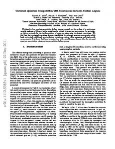
a directed acyclic graph. Each node v in the graph is labeled by a gate gv ∈ G of order (kv , lv ). The in-degree

and out-degree of v are equal kv and lv , respectively. Here is a schematic example of such a circuit. 6

6 6

g5

g4

6

6 6 g2 6 6 6 g1

6 6

g3 6 6

The circuit operates on a density matrix as follows: Definition 4. final density matrix: Let Q be a quantum circuit. Choose a topological sort for Q: gt ...g1 . Where gj are the gates used in the circuit. The final density matrix for an initial density matrix ρ is Q ◦ ρ = gt ◦ ... ◦ g2 ◦ g1 ◦ ρ. Q ◦ ρ is well defined and does not depend on the topological sort of the circuit [4]. At the end of the computation, the r output qubits are measured, and the classical outcome, which is a string of r bits, is the   output of the circuit. For an input string i, the probability for an output string j is hj| Q ◦ |iihi| |ji.

Definition 5. Computed function: Let Q be a quantum circuit, with n inputs and r outputs. Q is

said to compute a function f : {0, 1}n 7−→ {0, 1}r , with accuracy ǫ if for any input i ∈ {0, 1}n, the probability

for the output to be f (i) is greater than 1 − ǫ.

11

2.7. Quantum Circuits with probabilistic Errors. . To implement noise in the quantum circuits, we divide the quantum circuit to time steps, and the gates are applied at integer time steps. We permit that qubits are input and output at different time steps. Faults occur in between time steps, in the locations of the circuit. Definition 6. A set (q1 , q2 , ..ql , t) is a location in the quantum circuit Q if the qubits q1 , ...ql participated in the same gate in Q, in time step t. and no other qubit participated in that gate. For this matter, the absence of a gate is viewed as the identity gate on one qubit, so if a qubit q did not participate in any gate at time t, then (q, t) is a location in Q as well. Each location in the circuit exhibits a fault with with independent probability η. Definition 7. The list of times and places where faults had occurred, (in a specific run of the computation) is called a fault path. Each fault path, F , is assigned a probability P r(F ), which is a function of the number of faults in it. A

fault at time t at a certain location means that an (arbitrary) general quantum operation is applied on the

faulty qubits after time t. Given a certain fault path, we still have to determine the quantum operations that were applied on the faulty qubits. Denote by E(F ) the choice of faults for the fault path, say Et , ...E2 , E1 .

The final density matrix for this given choice E(F ) is easily defined by applying the faults in between the

gates: Q(F ) ◦ ρ = Et ◦ gt ◦ ...E2 ◦ g2 ◦ E1 ◦ g1 ◦ ρ. The final density matrix, Q ◦ ρ of the circuit is defined as a

weighted average over the final density matrices for each fault path: X Q◦ρ= (2.2) P r(F )Q(F ) ◦ ρ. F

This final density matrix depends on the exact choice of quantum operations applied on the faulty gates. However, a noisy quantum computer is said to compute a function f with confidence ǫ in the presence of error rate η, if the circuit outputs the function f with accuracy ǫ regardless of the exact specification of the quantum operations which occurred during the faults. 2.8. Quantum Circuits with General Local Noise. In most of the paper we will use only the probabilistic noise model described above. However, our result will be generalized in section 8 to a much more general noise model. In the general noise model, we replace the probabilistic faults which occur with probability η in each location by applying in each location in the quantum circuit an arbitrary general quantum operator, on which the only restriction is that it within η distance to the identity, in a certain norm of super-operators. Thus, in between time steps, a noise operator operates on all the qubits. For the time step t the noise operator is of the form

(2.3)

E(t) = EA1,t (t) ⊗ EA2,t (t) ⊗ · · · ⊗ EAlt ,t (t).

Ai,t runs over all possible locations at time t, and for each one of them, (2.4)

kEAi,t (t) − Ik ≤ η

The exact definition of the norm on super-operators is not used in this paper. We merely need the following properties: 12

1. kT ρk ≤ kT kkρk

2. kT Rk ≤ kT kkRk

3. kT ⊗ Rk = kT kkRk

4. The norm of any physically allowed super-operator T is equal to 1. A reasonable norm on super-operators should satisfy these properties. One example is the diamond norm suggested by Kitaev[39, 4]. 2.9. Connection to Specific Noise Processes. Independent and quasi independent probabilistic errors, amplitude and phase damping, decoherence, and systematic inaccuracies in gates, are all special cases of the general noise model defined above. For independent probabilistic errors, where an error E occurs

with probability η, we can write for each one of the super-operators in the product2.3: EAi,t (t) = (1 − η)IAi,t + ηE ′ Ai,t (t)

(2.5)

where E ′ Ai,t (t) is any physical super operator. This satisfies the conditions of local noise 2.3,2.4 with error rate 2η. This is true, in particular, also for probabilistic collapses of the wave function, a process in which

each qubit randomly collapses to one of its basis states, for a given basis (not necessarily the computational basis |0i, |1i). E ′ Ai,t (t) is then the physical super-operator which measures the qubit in the chosen basis.

Depolarization, in which a qubit is randomly replaced by a completely random qubit, i.e. a qubit in the identity density matrix, is also a special case of probabilistic noise, in which the super-operator E ′ Ai,t (t)

replaces all the qubits in Ai,t by completely random qubits. Decoherence[17], amplitude damping and phase damping[] are all special cases of interactions between the qubits and the environments, and as such they can be described in the above models by definition, as long as the process is local. Systematic inaccuracies in a given gate are described by applying the same noise operator on all locations where that gate operated. The generalizations described in the last subsection describe how to implement quasi independent probabilistic errors. 2.10. Adding correlations to the Noise Model. Two very important assumptions were made when introducing our general model of noise. • Locality: No correlations between environments of different qubits, except through the gates.

• The Markovian assumption: The environment is renewed each time step, and hence no correlations between the environments at different time steps.

Both of these assumptions can be slightly released, to allow exponentially decaying correlations in both space and time, while the results of this paper still hold. To add exponentially decaying correlations to the probabilistic noise model, we generalize it in the following way. Instead of considering independent probabilities for error in each location, we require that the probability for a fault path which contains k locations is bounded by some constant times the probability for the same fault path in the independent errors model: (2.6)

P r(f ault path with k errors) ≤ cη k (1 − η)v−k .

where v is the number of locations in the circuit. Then, an adversary chooses a noise operator which operates on all the qubits in the fault path, without any restrictions. The most general case is as follows. The adversary 13

adds some blank qubits, which are called the environment, at the beginning of the computation. Each time step, the adversary can operate a general operator on the environment and the set of qubits in the fault path at that time step. This model allows correlations in space, since the noise operator need not be of the form of a tensor product of operators on different locations. Correlations in time appear because the environment that the adversary added in not renewed each time step, so noise operators of different time steps are correlated. Note that the independent probabilistic noise process is a special case of this process. 3. Quantum Error Correcting Codes. Here we recall the definition of quantum codes, and of Calderbank-Shor-Steane (CSS) codes[13, 68]. These codes were first presented for qubits, that is over the field F2 . We give here a proof for the fact that CSS codes are quantum codes, which is significantly simpler than the original proof[13], and generalize it to Fp for any p > 2. On our way, we use the fact that it suffices to correct phase flips and bit flips, in order to correct general errors. This was first proved by Bennett et. al.[8], using a beautiful argument which involved the notion of group symmetry and a quantum operation called “twirl”. We give here a simple proof of this theorem, which uses merely linearity of quantum operators, and is based on an idea by Steane[68]. We then define a new class of quantum codes, which we call polynomial quantum codes. These are a special case of CSS codes over Fp . These codes are based on ideas by Ben-Or et. al.[9] who used random polynomials for distributed fault tolerant classical computation. This section assumes basic knowledge in classical error correcting codes, which can be found in [49]. 3.1. Quantum Codes. Definition 8. A [k, m]-quantum code is a subspace of dimension k in the Hilbert space of m qubits. A word in the code is any vector in the subspace, or more generally any density matrix ρ supported on the subspace. We say that the word had d errors in qubits q1 , ..qd if a general physical operator on these d qubits, E(q1 , ..qd ) was applied on ρ. A procedure R, i.e. a sequence of gates, is said to correct an error E(q1 , ..qd ) on ρ if

(3.1)

R ◦ E(q1 , ..qd ) ◦ ρ = ρ

Definition 9. Let C be a [k, m] quantum code. Let {|αi i}ki=1 be a basis for this quantum code. C is

said to correct d errors if there exists a sequence of quantum gates R, called an error correction procedure, which corrects any d errors on any d qubits, on any word in the code, i.e for any i, j and E(q1 , ..qd ) R ◦ E(q1 , ..qd ) ◦ |αi ihαj | = |αi ihαj |

Note that during the operation of R, it is allowed to use extra qubits, but at the end all ancillary qubits

are discarded, and the original state should be recovered.

3.2. From General Errors to Bit Flips and Phase Flips. A crucial and basic fact[8] in quantum error corrections is that it suffices to correct two basic errors, called bit flips and phase flips, in a small number of qubits, in order to correct a general error on these qubits. Our proof of this fact uses merely 14

linearity of quantum operators. Let us define basic errors as those in which one of the Pauli unitary operators occur: (3.2)

I=

1 0 0 1

!

, σx =

0

1

1

0

!

, σy =

0

1

−1 0

!

, σz =

1

0

0 −1

!

.

σx is called a bit flip, since it takes |0i to |1i and |1i to |0i. σz is called a phase flip, as it multiplies |1i by

a minus sign, while leaving |0i as is. σy is a combination of the two, since σy = σz σx . A basic error on d

qubits is obtained by taking tensor products of d of the above Pauli matrices. More formally, consider all possible strings e of length d in the alphabet I, x, y, z. The set of 4d matrices: (3.3)

σe = σed ⊗ · · · σe1 ,

e ∈ {1, x, y, z}d

is a basis for operators on the Hilbert space of d qubits. Before we show that it suffices to correct basic errors, we need two definitions: Definition 10. We say that R corrects basic errors of length d in C if for any two basis states of the

code, |αi and |α′ i, and any basic error of length d, σe we have (3.4)

R ◦ σe |αihα′ |σe† = |αihα′ |

Definition 11. We say that R detects basic errors of length d in C if for any two basis states of the

code, |αi and |α′ i, and any two different basic error of length d, σe 6= σe′ , (3.5)

R ◦ σe |αihα′ |σe†′ = 0

The reason for the fact that such R is said to detect errors is that indeed, if at the end of the procedure R

the error e is written down on an ancilla, R ◦ σe |αi = |αi ⊗ |ei, then for two different errors the two ancilla

states are orthogonal, and thus when discarding the ancilla qubits we get zero. In the rest of the paper, we will only use error correcting procedures which detect the errors. We can now prove the following: Theorem 1. Let C be a quantum code, and let R correct and detect any basic error of length d in C.

Then R corrects any general error on any d qubits in C.

Proof: We recall that any noise operator L from d to d′ qubits can be written as a combination of three

operators: adding d + d′ blank qubits, applying a unitary transformation on the 2d + d′ and discarding 2d qubits. The last operator which discards qubits will be denoted as T . Combining the first two operations,

we have in the most general case the following operation on d qubits. For all 0 ≤ i ≤ 2d − 1, (3.6)

|ii 7−→ |0

d+d′

i|ii 7−→

d 2X −1

j=0

|Aji i ⊗ |ji

where all the coefficients are put into the vectors |Aji i which are not unit vectors. We now use the fact that the

basic errors,σe, on d qubits form an orthonormal basis with respect to the inner product (V, U ) =

1 2d tr(V

U †)

for 2d × 2d matrices. We define A, a vector of matrices, or a matrix with entries which are vectors, by 15

Ai,j = |Aji i. For any basic error vector e of length d, define |Ae i = (A, σe ) = 12 tr(A · σe† ), where A should be

thought of as a vector of matrices, and thus Aσe† is also a vector of matrices, the trace of which is a vector. P P Due to the fact that the basic errors are orthonormal, we have that j |Aji i ⊗ |ji = e |Ae i ⊗ σe |ii, or equivalently the two first steps of the noise operator can be written as: X L= |Ae ihAe′ | ⊗ σe · σe†′ (3.7) e,e′

Now, R will indeed correct E = T ◦ L, by the following: X X |Ae ihAe′ | ⊗ σe |αihα′ |σe†′ = (T ◦ (3.8) R ◦ E ◦ |αihα′ | = R ◦ T ◦ |Ae ihAe |) ⊗ |αihα′ | = |αihα′ | e

e,e′

where in the second equality we have used the fact that T commutes with R because they operate on different P e |Ae ihAe | = c

qubits, and that R corrects and detects errors. In the last equality we used the fact that T ◦

does not depend on |αi, |α′ i. Choosing |αi = |α′ i, Tr(R ◦ E ◦ |αihα|) = Tr(c|αihα|) = c, but on the other

hand R ◦ E is trace preserving so c = 1. 2

3.3. Calderbank-Shor-Steane Codes. We give here the definition of CSS codes, which is slightly modified from the definition in [13]. A linear code of length m and dimension k is a subspace of dimension k in F2m , where F2m is the m dimensional vector space over the field of F2 of two elements. Let C1 , C2 be linear code such that {0} ⊂ C2 ⊂ C1 ⊂ F2m , and let us define a quantum code by taking the superpositions of all words in a coset of C2 in C1 to be one basis word in the code. We have:

(3.9)

X 1 |w + ai. ∀a ∈ C1 /C2 : |Sa i = √ 2dim(C2 ) w∈C2

Note that |Sa i is well defined and does not depend on the representative of the coset since if (a1 − a2) ∈ C2

then |Sa1 i = |Sa2 i. Also, for different cosets the vectors are orthogonal, because if (a1 − a2) 6∈ C2 , then

hSa1 |Sa2 i = 0. Thus, this defines a basis for a subspace of dimension 2dim(C1 )−dim(C2 ) , which is our quantum

code. Note that the support of |Sa i are words in the code C1 . We will see that bit flips can be corrected

using classical error correction techniques for the code C1 . Before we discuss how to correct phase flips, let

us define a very important quantum gate on one qubit, called the Hadamard gate, or the Fourier transform over F2 : (3.10)

H=H

−1

√1 2 √1 2

=

√1 2

− √12

!

Observe that Hσz H −1 = σx

(3.11)

meaning that a phase flip transforms to a bit flip in the Fourier transform basis. Applying the Hadamard gate on each qubit in |Sa i, we get the state: 1

(3.12) |Ca i = H ⊗ H ⊗ · · · ⊗ H|Sa i = √ 2m+dim(C2 )

m 2X −1

b=0

16

X 1 (−1)a·b |bi (−1)(w+a)·b |bi = √ m−dim(C2 ) 2 ⊥ w∈C2 b∈C X

2

which is a superposition of words in C2⊥ , and so to correct phase flips, one transforms to the Fourier basis and corrects bit flips in the code C2⊥ . These ideas lead to the following theorem by Calderbank and Shor[13]. We give here a simple proof of this theorem, based on theorem 1. Theorem 2. Let C1 and C2⊥ be linear codes over F2 , of length m, such that 0 ⊂ C2 ⊂ C1 ⊂ F2m ,

and such that C2⊥ , C1 can correct t errors. Then the subspace spanned by |Sa i for all a ∈ C1 /C2 is a [2dim(c1 )−dim(C2 ) , m] quantum code which can correct t errors. The error correction procedure, R, is con-

structed by correcting pit flips with respect to C1 in the S-basis, rotating to the C-basis by applying Fourier transform bit-wise, correcting with respect to C2⊥ and rotating back to the S-basis. Proof: We define the procedure RC1 to be a unitary embedding of m qubits to 2m qubits, by RC1 |ii = |wi ⊗ |ei

(3.13)

for each i ∈ F2m , where w ∈ C1 is a string of minimal distance to i, and e ∈ {0, 1}m satisfies w + e = i.

Since this is a one to one transformation, it is a unitary embedding, and is a possible quantum operator. Let eb ∈ {0, 1}m have at most t 1′ s. Let Eb be an error operator which is a tensor product of bit flips (σx ) where eb is one and identity on the other coordinates. Then for any |αi, |α′ i supported on C1 we have RC1 ◦ Eb ◦ |αihα′ | = |αihα′ | ⊗ |eb iheb |

(3.14) RC2⊥ is defined similarly: (3.15)

RC2⊥ |ji = |wi ⊗ |ei

where w ∈ C2⊥ is a string of minimal distance to j, and e ∈ {0, 1}m satisfies w + e = j. Let ef ∈ {0, 1}m

have at most t 1′ s (ef for phase flips.). Let Ef be an error operator which is a tensor product of phase flips

(σz ) where ef is one and identity on the other coordinates. Then for any |βi, |β ′ i supported on C2⊥ we have (3.16)

RC2⊥ ◦ Ef ◦ |βihβ ′ | = |βihβ ′ | ⊗ |ef ihef |

Denote by H the operator of applying H on every qubit: H = H ⊗ H ⊗ · · · ⊗ H. We claim that the operator (3.17)

R = Tf ◦ Tb ◦ H ◦ RC2⊥ ◦ H ◦ RC1

is the desired error correcting procedures. Tf , Tb are the operators discarding the qubits added for RC2⊥ , RC1 , respectively.

By theorem 1, it is enough to show that this procedure corrects and detects d basic errors. To show that it corrects d basic errors, write the error vector e in two parts, eb and ef as follows: eb will be 1 in the coordinates where σx or σy occurred, and 0 elsewhere. ef will be 1 in the coordinates where σz or σy occurred, and 0 elsewhere. We can therefore write the error operator E as a product of two operators, E = Eb Ef . Now, using, in the following order, equation 3.17, the fact that RC1 commutes with Ef , equation 3.14,3.11 and 3.16, we have the desired result:

(3.18)

R ◦ E ◦ |αihα′ | = Tf ◦ Tb ◦ H ◦ RC2⊥ ◦ H ◦ Ef ◦ RC1 ◦ Eb ◦ |αihα′ | = 17

Tf ◦ Tb ◦ H ◦ RC2⊥ ◦ H ◦ Ef ◦ |αihα′ | ⊗ |eb iheb | =

Tf ◦ H ◦ RC2⊥ ◦ H ◦ Ef ◦ |αihα′ | =

Tf ◦ H ◦ RC2⊥ ◦ (H ◦ Ef ◦ H) ◦ (H ◦ |αihα′ |) =

Tf ◦ H ◦ (H ◦ |αihα′ |) ⊗ |ef ihef | = |αihα′ |.

It is left to show that R also detects d basic errors. This follows from the fact that if e 6= e′ , then either

ef 6= e′f or eb 6= e′b . Now reducing two orthogonal vectors gives zero, i.e. if eb 6= e′b Tb ◦ |eb ihe′b | = 0 and if

ef 6= e′f Tf ◦ |ef ihe′f | = 0. 2.

3.4. CSS codes over Fp . The theory of quantum error corrections can be generalized to quantum computers which are composed of quantum particles of p > 2 states, called qupits. To generalize the notion of bit flips and phase flips to qupits define the following two matrices: • B: • P :

where w = e

B|ai = |(a + 1)mod pi

P |ai = wa |ai

2πi p

. We will consider combinations of powers of these matrices, i.e. the p2 matrices, ′

BcP c ,

(3.19)

∀c, c′ ∈ Fp .

This set can be easily seen to be an orthonormal basis for the set of p × p complex matrices, with the inner

product (U, V ) = 1p tr(U B † ). Like in the case of qubits, errors of type B transform to errors of type P and vice versa, via a Fourier transform, which is defined to be 1 X ab W : |ai 7−→ √ w |bi. p

(3.20)

b∈F

And it can be easily checked that ∀c ∈ Fp , W P c W −1 = B c , W B c W −1 P c

(3.21)

We can therefore define CSS codes over Fp . The statements and proofs of theorems 1 and 2 are generalized to Fp using the above definition of bit flips and phase flips, where F2m is replaced by Fpm and Hadamard gate is replaced by the Fourier transform W over Fp everywhere. 3.5. Polynomial Quantum Codes. We define polynomial codes over Fp . Set d to be the degree of the polynomials we are going to use, and set m to be the length of the code. p > m will be the number of elements in the field Fp we will be working with. Set α1 , ...αm to be m distinct non zero elements of the field Fp . Define the linear codes: (3.22)

C1 = {(f (α1 ) · f (αm ))|f (x) ∈ F (x), deg(f (x)) ≤ d} ⊂ Fpm C2 = {(f (α1 ) · f (αm ))|f (x) ∈ F (x), deg(f (x)) ≤ d, f (0) = 0} ⊂ C1

We can now define the quantum code: (3.23)

1 ∀a ∈ C1 /C2 , |Sa i = p pd

X

f ∈V1 ,f (0)=a

18

|f (α1 ) · · · f (αm )i

Clearly, C2 has p different cosets in C1 , and so C1⊥ has p disjoint cosets in C2⊥ . Thus the dimension of the code is p, and the code encodes exactly one qupit. Note that this code is a special case of CSS codes, which will be used to prove the following theorem: Theorem 3. A polynomial code of degree d with length m over Fp is a [p, m] quantum code which corrects ⌋, ⌊ d2 ⌋} errors. min{⌊ m−d−1 2 Proof: Two different words in C1 agree on at most d coordinates, and thus C1 is a linear code of distance m − d. It can thus correct and detect ⌊(m − d − 1)/2⌋ errors. C2⊥ is a linear code of minimal distance ≥ d + 1.

This is true since the projection on any d coordinates of the code C contains all possible strings of length d, and therefore the only vector of length d orthogonal to all the vectors is the 0 vector. Thus, C2⊥ corrects and detects ⌊d/2⌋ errors. Theorem 3 follows from theorem 2. 2 4. Computing on States Encoded by CSS codes. CSS codes will be used to perform computations fault tolerantly: The idea is to compute on quantum states encoded by CSS codes. Each gate is replaced by a procedure which imitates the operation of the gate on the encoded states. In order for the computation to be fault tolerant, the procedures have to be designed in such a way so that a small number of errors during the procedure cannot propagate to too many errors at the end of the procedure, before error correction can be applied. The basic definitions are given next. We then show how to perform fault tolerant operations on states encoded by CSS codes. We follow Shor’s constructions very closely, with some additional tricks and modifications mainly in the construction of the ancilla state required for the Toffoli gate, and in the decoding and error correction procedures. These modifications are done in order to avoid measurements and classical operations during the computation. In fact, this is the only difference between the results presented in this section, and the results derived by Shor in []. 4.1. Fault Tolerant Procedures on Encoded States- General Definitions. Say we have a unitary gate g which was applied on the state |αi in the original circuit. We now want to apply a sequence of gates,

or a “procedure”, P (g), on the state encoding |αi, such that P (g) will take the encoded |αi to the state

encoding g|αi.

Definition 12. A sequence of gates P (g) is said to encode a gate g for the code C if for any superposition |αi, P (g)|S|αi i = |Sg|αi i. We will want P (g) to be such that an error occurring at one gate or qubit during the procedure will not affect too many qubits at the end of the procedure, so that the error can be corrected. A location (q1 , ..ql , t) effects a qubit q ′ at time t′ > t if there is a path in the circuit from (q1 , ..ql , t) to (q ′ , t′ ). Definition 13. The “spread” of a procedure is the maximal number of qubits in one block in the output of the procedure, which are effected by one location in this procedure. If we use only procedures with small spread, the error corrections will still be able to correct the damage using the undamaged qubits, provided that not too many errors happened during the procedure. The notion of reduced density matrices is useful here: At the end of a fault tolerant procedure which operates on a state |αi, the result will be “correct” on all qubits except those effected by the fault. This

means that the reduced density matrix on all the qubits except those which where effected, is the same as 19

it would have been if no fault occurred at all. 4.2. Questions of Ancilla Qubits. In some of the procedures, we will use ancilla qubits, as extra working space. At the end of the procedure these qubits will be discarded, in order to get exactly the state we need. As was explained in subsection 2.3, we will always discard qubits which are in tensor product with the rest of the system, so the operation of discarding means simply erasing their state, and the resulting state is a pure state. This is necessary if we want to operate unitary operations on the encoded states. We will describe a procedure by specifying what it does to basic states of the code. It is easy to see that if for any input basis state, the state of the ancilla qubits at the end of the procedure are in a tensor product with the rest of the qubits, and their state does not depend on the input basis state, i.e. (4.1)

|Sa i 7−→ |Sg(a) i ⊗ |Ai

where A is independent of a, then for any input superposition for the procedure the ancilla qubits will be in tensor product with the rest of the qubits, and thus they can be discarded simply by erasing them. This requirement of independence of the ancilla qubits on the basis state can be released in two cases. An encoding procedure, is the procedure which takes a block of input bits, 0m to the state encoding 0, |S0 i,

and likewise for 1. For the encoding procedure, we know that the procedure always gets as an input a basis state. Thus, we release the above requirement, and demand only that the ancilla state is in a tensor product with the computational qubits when the input to the procedure is a basis state. (The ancilla might therefore depend on the input, and indeed it will, but we are allowed do discard it anyway.) The requirement of tensor product with the ancilla can also be released in the decoding procedure, since the state will not be used any more, and we should only check that it gives the correct answer when measured. It suffices to check the independence of the ancilla in the case of no fault in the procedure. The fact that the procedures are fault tolerant guarantees that even if a fault occurred, the reduced density matrix of the non-effected qubits is just like in the case in which no fault occurred at all. 4.3. Some Restrictions on the CSS Codes. In the following, we will put some restrictions on the CSS codes which we will use. This is done in order to be able to apply several gates fault tolerantly bitwise, as will be seen shortly. We require that C1 is a punctured doubly even self dual code, and that C2 = C1⊥ . A punctured code is a code which is obtained by deleting one coordinate from a code C ′ , and a punctured self dual code means that we require in addition that C ′ is self dual, i.e. C ′ = C ′⊥ . We also require that C ′ is a doubly even code, i.e. the weight of each word in the code is divisible by 4. To see that C2 = C1⊥ ⊂ C1 , as

in the definitions of CSS codes, observe that if v ⊥ C1 , then v0 ⊥ C ′ so v0 ∈ C ′⊥ = C ′ , so v ∈ C1 . We will

denote C1 = C, and C2 = C ⊥ .

We now claim that there are only two cosets of C ⊥ in C. If the length of C is m, then dim(C ′⊥ ) = dim(C ′ ) = (m + 1)/2. Hence dim(C) = (m + 1)/2 as well, since |C| = |C ′ |, because no two words in C ′ are

mapped to the same word in C by the punctuation. Hence, dim(C ⊥ ) = m − (m + 1)/2 = (m − 1)/2 and so dim(C) − dim(C ⊥ ) = 1. Observe that C includes the all one vector: ~1 ∈ C. This is true since 1m+1 ∈ C ′⊥ ,

because C ′ is even, and since C ′ is self dual, 1m+1 ∈ C ′ . Hence 1m ∈ C. Observe also that the length m must be odd due to the above considerations. This implies that ~1 6∈ C ⊥ . The two code words in our 20

quantum code can thus be written as |S~0 i =

(4.2)

|S~1 i =

X

w∈C ⊥

X

w∈C ⊥

|wi |w + ~1i

|S~0 i,|S~1 i, can be thought of as encoding |0i, |1i respectively. We will make use of the fact that ~a ·~b mod 2 = −−−→ ab, for a, b ∈ 0, 1, and that ~a + ~b = a + b. This fact allows us to shift easily between operations on vectors, and operations on the bits they represent. We will therefore usually omit the vectors in the notations of |S~0 i and |S~1 i, unless there is ambiguity.

4.4. The Set of Gates for CSS codes. We work with the following set of gates, which we denote by G1 : 1. Not: |ai 7−→ |1 − ai,

2. Controlled not: |a, bi 7−→ |a, a + bi, 3. Phase rotation: |ai 7−→ ia |ai,

4. Controlled Phase rotation: |ai|bi 7−→ (−1)ab |ai|bi, P 5. Hadamard: |ai 7−→ √12 b (−1)ab |bi, 6. Toffoli gate: |a, b, ci 7−→ |a, b, c + abi, 7. Swap |ai|bi 7−→ |bi|ai,

8. Adding a qubit in the state |0i,

9. Discarding a qubit.

where all the addition and multiplication are in F2 (i.e. mod 2). We will show later on that this set of gates is universal. We remark here, that G1 is by no means a minimal universal set of gates, but the fault

tolerant procedures become simpler and shorter if we have a larger repertoire of fault tolerant gates that we can use. The following theorem shows how to perform gates from G1 on encoded states fault tolerantly.

Theorem 4. There exists fault tolerant procedures which simulate the operations of all the gates from G1 ,

on states encoded by punctured self dual doubly even CSS codes such that one error in a qubit or a gate effects at most four qubits in each block at the end of the procedure. There exist such procedures also for encoding, decoding and error correction. Moreover, all these procedures use only gates from G1 , and in particular do not use measurements.

To prove the theorem, we first show this for the gates which can be applied bit-wise, then for the encoding, decoding and error correction procedures, and then for the rest of the gates. 4.5. Bitwise Fault Tolerant Procedures. Let g be a gate on k qubits. A bitwise procedure of this gate is defined by labeling the qubits in each one of k blocks from 1 to m, and then applying the gate m times, each time on all qubits with the same label. Obviously, an error in this procedure can effect only one qubit. All the gates in G1 can be applied bitwise, except the Toffoli gate and the gate which adds a blank qubit. These are the NOT, Controlled not, Phase rotation, Controlled Phase rotation, Hadamard, Swap and Discarding a qubit. This is trivial for the SWAP gate, and the gate which discards a qubit. Simple 21

calculations show this also for the other gates. In the following we omit overall normalization factors, since all vectors are known to be unit vectors. We also set a, b ∈ C/C ⊥ . (4.3)

|Sa i =

X

w∈C ⊥

|a1 + w1 i ⊗ ...|am + wm i 7−→

X

w∈C ⊥

|a1 + 1 + w1 i ⊗ ...|am + 1 + wm i = |Sa+~1 i

For CNOT, (4.4) |Sa i|Sb i =

X

w∈C ⊥

X

w∈C ⊥

|a1 + w1 i ⊗ ...|am + wm i |a1 + w1 i ⊗ ...|am + wm i

= |Sa i|Sa+b i

X

w ′ ∈C ⊥

X

w ′ ∈C ⊥

′ |b1 + w1′ i ⊗ ...|bm + wm i 7−→ ′ |a1 + b1 + w1 + w1′ i ⊗ ...|am + bm + wm + wm i

where the last equality follows from the fact that C ⊥ is a linear subspace, and therefore summing over w + w′ for a fixed w in the code is equivalent to summing over w′ . For the Phase gate, apply the gate |ai 7−→ ia |ai three times on each coordinate. This gives

(4.5)

|Sa i =

X

w∈C ⊥

X

|a1 + w1 i ⊗ ...|am + wm i 7−→

i3(

w∈C ⊥

P

k

ak +wk )

|a1 + w1 i ⊗ ...|am + wm i.

This is the desired result, because C is a punctured doubly even self dual code, and it is easy to check that all words in C ⊥ have weight which is divisible by 4, and all words in C but not in C ⊥ have weight which is 3 mod 4. For the encoded controlled phase gate, (4.6)

|S~a i|S~b i =

X

w,w ′ ∈C ⊥

|~a + wi|~b + w′ i 7−→

X

w,w ′ ∈C ⊥

′ ~ (−1)(~a+w)·(b+w ) |~a + wi|~b + w′ i

Now, (~a + w) · (~b + w′ ) = ~a · ~b mod 2. This is true since ~a ∈ C and w′ ∈ C ⊥ so ~a · w′ = 0 mod 2, and likewise w · ~b = w · w′ = 0 mod 2. Moreover, ~a · ~b mod 2 is equal to ab, and so the final state is indeed the desired state. Finally, for the Hadamard gate,

(4.7)

|Sa i = =

X

w∈C ⊥

X

x∈C

|a1 + w1 i ⊗ ...|am + wm i 7−→ a·x

(−1)

|xi =

X

X

x∈F2m

X

w∈C ⊥

a·(b+w)

(−1)

b∈C/C ⊥ w∈C ⊥

X

(−1)(a+w)·x |xi =

|b + wi =

X b

(−1)a·b |Sb i.

4.6. Fault Tolerant Error Correction Procedure for CSS Codes. So far, we have described how to apply those procedures which can be obtained by bitwise operations. Before we continue to the Toffoli gate and the gate which adds a blank qubit, we first show how to apply encoding, decoding and error correction fault tolerantly. These procedures will be used later in the remaining of the gates. We now construct the error correction procedure. It is composed from detecting and correcting bit-flips, using classical error correction techniques for the code C, rotating by Hadamard gate to the C−basis, and correcting bit-flips using again classical error correction techniques. Finally we rotate back by applying Hadamard bit-wise. 22

We now describe how to correct bit-flips. For this, we recall that for linear classical codes over F2 , one can define the parity check matrix H of the code C. The kernel of H is exactly the words in C. If an error occurred in a word w, the new word can be written w + e, where e is called the error vector. H(w + e) = He = s is called the syndrome of the error, and given the syndrome s, one can find the error vector of minimal weight which gives s. The error correction is therefore done by first finding the syndrome, and then deducing the error vector from it. We now want to compute the j ′ th bit of the syndrome fault tolerantly. This is simply the inner product of the j ′ th row of H with the word. If out computation was noiseless, we could do the following: we apply CNOT from the block we are correcting to one blank qubit, only on the coordinates which are 1 in the j ′ th row of the parity check matrix of the code. This will compute the inner product of the word we are correcting with the j ′ th row of the parity check matrix, and the extra blank qubit will thus contain the j ′ th bit of the syndrome. However, this is not a fault tolerant procedure, since an error in one of the CNOT gates causes an error in the extra qubit, which propagates through the other CNOT gates to other qubits in the block. To avoid this problem, we will use an ancillary state on l qubits: 1

(4.8)

2

(l−1) 2

X

b;b·~1

|bi

where l is the number of 1′ s in the in the j ′ th raw of H, the parity check matrix of C ⊥ . This state is actually the superposition of all states with an even number of 1’s. It can be easily constructed by starting with |0l i,

applying Hadamard on the first qubit and then CNOT from this qubit to all the other l − 1 qubits, to get

the “cat state” on l qubits, (4.9)

1 |catl i = √ (|0l i + |1l i). 2

and then rotating each qubit of the cat state to get the desired state. We would now like to apply CNOT bitwise from the block we are initializing to the cat state only on the coordinates which are 1 in the j ′ th row of the parity check matrix. Then we apply a classical computation, using only gates from G1 , on the ancilla state, to find out the parity of the strings in the ancilla state, and

write this parity on another qubit, initialized in the state |0i. The resulting state will be the j ′ th syndrome bit.

The only problem in this scheme is that the generation of the cat state is not done fault tolerantly, and thus one error can cause the entire cat state to be ruined; The CNOT gates will then propagate this error to many qubits in the block. The solution to this problem is to verify that the cat state is indeed a superposition of the two states |0l i and |1l i, before continuing. The relative phase between the two states can still be mistaken, but this will not cause any error to propagate to the state by the CNOT gates, but

only cause the syndrome to be mistaken. To see this, suppose we have instead of the cat state, the state c0 |0i + c1 |1i. This state transforms after the Hadamard gates to the state: (4.10)

c0

X i

|ii + c1

X

23

i

~

(−1)i·1 |ii

Now, consider applying CNOT’s on all the 1 coordinates in the parity check matrix from a correct encoded P state to i |ii. This is simply the identity operator: X X (4.11) |ii |ii 7−→ (c0 |S0 i + c1 |S1 i) (c0 |S0 i + c1 |S1 i) i

i

and the same for the other term

P

i·~1

i (−1)

|ii. This means that in spite of the fact that the cat state is not

correct, this does not cause any error in the original state.

This verification was done by Shor[64] using measurements and assuming noiseless classical computation, by measuring the XOR of pairs of the qubits. If we want to avoid measurements, we proceed as follows. We now want to compute whether the bits in the cat state are all equal. For this, note that checking whether two bits are equal, and writing the result on an extra blank qubit, can be easily done by a small circuit which uses Toffoli and NOT gates. We denote this circuit by S, and also denote the qubits in the cat state by 1, ...l. We add l − 1 extra blank qubits, and apply the circuit S first from each even pair of qubits (e.g. the pair of qubits (1, 2), (3, 4)...), to one of the blank qubits; Then apply S from each odd pair of qubits

(e.g. the pairs (2, 3), (4, 5)...) to one of the remaining blank qubits. We get l − 1 qubits which are all 1, if no

error occurred, indicating that all the qubits are equal. We then apply a classical circuit on all these qubits, which checks whether they are all 1, and write the result on an extra blank qubit, which is our check bit, and indicates that all the bits in the cat state are equal. We now want to use the cat state, but condition all the operations on the fact that the check bit is indeed 1. However, if we do this, an error in the check bit, might propagate to all qubits in the state we are trying to correct. Hence, to keep the procedure fault tolerant, we construct m different check bits, one for each qubit in the state we are correcting. This is done using m(l − 1) blank qubits, and applying all the operations above, where each operation is repeated m times. to

m different target qubits. Thus, we can verify that the cat state is of the form c0 |0i + c1 |1i, fault tolerantly.

We can now condition all the operations done in the syndrome measurement involving the i′ th qubit, on the i′ th check bit.

From the syndrome s we can compute the error vector e which is the vector of minimal weight which gives He = s. This can be done by classical operations, and need not be done fault tolerantly. Applying a CNOT from the result bit ei to the i’th bit will correct a bit flip in the i′ th bit. Now, we do not correct all qubits according to the error vector computed from one copy of the syndrome, since an error during the computation of the error vector might result in the entire error vector being mistaken, and the procedure will not be fault tolerant. Instead, we compute the syndrome independently m times, and from the i′ th copy of the syndrome we compute ei , from which we apply a CNOT to the i′ th bit of the state which we are correcting. The fact that for each bit we compute the syndrome independently ensures us that the procedure is fault tolerant. To apply error correction, we first apply error corrections of bit flips, according to the code C. We then apply a Hadamard gate to transform to the C-basis, and correct bit flips again, according to the code C. Then, we apply a Hadamard gate again, to get back to the S-basis. In all the procedures we have described so far, one fault causes at most one error in each block. Unfortunately, the propagation of errors in the error correction procedure is much worth. One fault in one of the circuits S, checking whether two qubits in the cat state are the same, might cause four qubits in this cat 24

state to be contaminated, where their check bits might still indicate a green light for following procedures. Hence, during the error corrections, each one of the four errors can propagate to the one qubit which is conditioned upon it. Apart from this bottle neck, all other errors have exactly one spread. 4.7. Fault Tolerant Encoding Procedure for CSS codes. An encoding procedure takes (4.12)

|0m i 7−→ |0m i|S0 i

|1m i 7−→ |1m i|S1 i

To construct this procedure fault tolerantly, it is enough to generate a state |S0 i fault tolerantly. This suffices

since given a string of bits, |0m i or |1m i, we first generate |S0 i and then apply a controlled not bitwise from

the given input string to the encoded state |S0 i.

To generate the state |S0 i, start with m blank qubits, |0m i, then apply an error correction procedure

with respect to a code which consists of one word: |S0 i alone. This is done by first applying Hadamard

gates bitwise on |0m i, and then correcting bit flips according to the code C ⊥ . To see that we indeed get the P2m −1 state |S0 i, note that after the first rotations we have i=0 |ii. The corrections will then take this state to

a uniform distribution over all the basic states in C ⊥ , due to the linearity of the code.

4.8. Error Correction which Projects any Word into the Code. We would like to insert here one important modification, which is not necessary for the fault tolerant error correction, but will become crucial when applying the error corrections in the recursive scheme. This is the requirement that the error correction takes any word to some word in the code, regardless of the number of faults. Roughly, this is done by checking whether too many errors occurred, and if so replacing the entire block by another block which is initialized in the state |S0 i. However, we should be careful to keep the procedure fault tolerant. We do

this in the following way: Before starting the correction procedure, we generate another state |S0 i on ancilla

qubits, as in the encoding procedure. When computing from the i′ th copy of a syndrome whether the i′ th

qubit is wrong, also compute whether the number of faults according to the syndrome is smaller than d, and write the answer on another qubit. The CNOT which checks if the i′ th bit is wrong and if so applies N OT on the i′ th qubit, is replaced by a Toffoli gate which also checks if the number of faults is smaller than d. We then swap the i’th qubit with the i′ th qubit of the state |S0 i, conditioned that the number of faults is

indeed larger that d. To achieve a swap between the second and third qubit conditioned on the first qubit, apply three Toffoli gates one after the other, where the target of the first gate is the third qubit, the target of the second gate is the second qubit and the target of the third gate is again the third qubit, i.e. (4.13)

Controlled(a)SW AP (b, c) = T (a, b, c)T (a, c, b)T (a, b, c)

which is easy to check. To see that this procedure indeed takes any word to some word in the code, observe that this is true if no error occurs in the procedure itself, and since the procedure is fault tolerant, the final state will differ from a word in the code only in the qubits effected by an error. 4.9. A Fault Tolerant Decoding Procedure for CSS codes. A decoding procedure applies (4.14)

|Sa i 7−→ |Aa i|~ai 25

where the state |Aa i is an ancillary state which depends on a. (We can discard this state at the end of the

procedure; we will see that whenever the decoding procedure is applied, the state encodes a well defined logical bit a. ) To apply this transformation, we compute a independently m times from the state |Sa i.

To do this, we add m2 blank qubits, and copy each qubit from |Sa i m times to m different blank qubits,

using m CNOT gates. We get m “copies” of |Sa i. (These of course are not really copies of |Sa i, since they

are entangled. However, each word in the classical code is copied m times.) On each copy of the word we apply the quantum analog of the classical computation that computes what is the logical bit that the word encodes. The answer, which is a if no error occurred, is written on another blank qubit. For this computation we use Toffoli, CNOT and NOT gates. We might need some extra blank qubits as working space. The computation of a is done is the shortest way possible, regardless of whether it is fault tolerant; An error in this computation can effect only the one copy of a which it computes. A fault in the first stage of copying the qubits m times can only effect one qubit in each of the copies, and if the number of errors in Sa plus number of faults in the first stage is smaller than the number of errors correctable by the code, these faults have no effect. One fault in the second stage of the procedure, during the computation of one of the a’s, can effect only the correctness of that a. 4.10. Toffoli Gate. To apply the Toffoli gate, we roughly follow Shor’s scheme, where we construct an ancillary state and use it to obtain the Toffoli gate. The main difference from Shor’s scheme is in the construction of the ancillary state, which is not completely straightforward if one wants to avoid using measurements. The following construction involves many details, and has no underlying structure, as far as we can see. As we will see in the next section, the Toffoli gate on polynomial codes can be applied in a much easier and shorter way. However, for completeness, we also give the details of the Toffoli procedure in the case of CSS codes. 4.10.1. Construction of the Ancilla state |Ai. We would now like to show how to construct the

state

(4.15)

|Ai =

1 |S0 S0 S0 i + |S0 S1 S0 i + |S1 S0 S0 i + |S1 S1 S1 i. 2

This will be done using the help of the encoded cat states. We will need the definition of the state (4.16)

|Bi =

1 |S0 S0 S1 i + |S0 S1 S1 i + |S1 S0 S1 i + |S1 S1 S0 i. 2

which is easily convertible to |Ai by applying an encoded NOT on the third block. The idea is that (4.17)

1 √ (|Ai + |Bi) 2

is actually very easy to construct, because it is equal to (4.18)

1 √ (|S0 i + |S1 i)(|S0 i + |S1 i)(|S0 i + |S1 i) 2 2

which can be constructed easily from 3 block of m blank qubits by applying an encoding procedure and then an encoded Hadamard gate on each block. In order to convert this state to |Ai, we use encoded cat states. 26

An encoded cat state, 1 |Scat i = √ (|S0 im + |S1 im ) 2

(4.19)

is also easy to construct fault tolerantly, in the following way: Generate m |S0 i states, |S0 im , fault tolerantly, using the encoding procedure on m blocks each containing m blank qubits. Then, apply an encoded

Hadamard gate on the first block, and then copy this block to all the other blocks by applying encoded CNOT from the first block to all other blocks. This results in an encoded cat state. We now apply fault tolerant error corrections on each block. Now, consider the transformation |S0 im |Ai 7−→ |S0 im |Ai

(4.20)

|S1 im |Ai 7−→ |S1 im |Ai

|S0 im |Bi 7−→ |S0 im |Bi

|S1 im |Bi 7−→ −|S1 im |Bi

If we can apply this transformation fault tolerantly, we could start with the state (4.21)

1 (|S0 im + |S1 im )(|Ai + |Bi) 2

and apply the transformation 4.20 to get

(4.22)

1 1 (|S0 im + |S1 im )|Ai + (|S0 im − |S1 im )|Bi 2 2

We might then be able to compute fault tolerantly in which of the cat states 12 (|S0 im ± |S1 im ) the ancilla is, and apply a NOT on the third block of |Bi, conditioned that the result is the second state 12 (|S0 im − |S1 im ).

Let us refer to this process as a “measurement” of the cat state, though no measurement will be involved. The transformation 4.20 can be done by applying (4.23)

|Sa i|bi|ci|di 7−→ (−1)a(bc+d) |Sa i|bi|ci|di

on the i’th block in the encoded cat state and the i’th bit in each of the three blocks of |Ai + |Bi. Note that transformation 4.23 need not be fault tolerant, and it might ruin the entire block |Sa i. Applying

transformation 4.23 for 1 ≤ i ≤ m it is easy to check that we get (4.24)

|Sa im |Sb i|Sc i|Sd i 7−→ (−1)a(bc+d) |Sa im |Sb i|Sc i|Sd i

which exactly achieves transformation 4.20. We now run into the problem of how to measure the encoded cat state. To solve this problem, we use three encoded cat states, instead of one, and repeat everything that we did on the first encoded cat state also for these states. The resulting state is 27

1 1 (|S0 im + |S1 im )3 |Ai + (|S0 im − |S1 im )3 |Bi 2 2

(4.25)

Now it becomes possible to measure the triple cat state, using majority. This can be done in several ways. One way is to apply encoded Hadamard gates on all blocks of the encoded cat states, which takes the encoded states into superpositions of encoded states, with certain parity: m

1 1 √ (|S0 im + |S1 im ) 7−→ √ 2 2m−1

(4.26)

2 X

i=0,i·~1=0

|Si1 i|Si2 i...|Sim i,

m

1 1 √ (|S0 im − |S1 im ) 7−→ √ 2 2m−1

2 X

i=0,i·~1=1

|Si1 i|Si2 i...|Sim i

To compute the parity fault tolerantly, we compute from each block the bit it represents, decoding it fault tolerantly. Then independently compute the parity of the m i′ th bits in the m blocks. The parity can be computed using Toffoli, CNOT and NOT gates. We now have m parity bits, for each encoded cat state. We compare them bitwise by applying on the three i’th parity bits and an ancilla bit a majority vote |a, b, c, di 7−→ |a, b, c, d + maj(a, b, c)i

(4.27)

which can be constructed from Toffoli, CNOT and NOT gates, since they are universal for classical computations. Now, apply CNOT bitwise from the resulting majority votes of the parity bits to the qubits in the third block of |Ai. It is left to see that one error in this procedure effects only one qubit in |Ai. We will consider errors

in different stages of the procedure. The construction of an encodes cat state id fault tolerant since it is

composed of the fault tolerant encoding procedure, and bitwise CNOT’s. The construction of the state √1 (|Ai 2

+ |Bi) is fault tolerant because we only used the fault tolerant encoding procedure and the fault

tolerant encoded Hadamard gate. A problem arises in transformation 4.20. During this transformation, an error can cause the entire block |Sa i to be ruined. Hence, an error during this transformation can cause a

whole block in one of the cat states in the state (4.25) to be effected, together with one qubit in each one of the last 3 blocks. However, one such block can ruin the parity bits of only one encoded cat state, and as long as the other two are still fine, the majority vote will still give the correct parity. An error in the parity computations or in the majority vote cannot effect more than one qubit in |Ai, since they are done bitwise.

This concludes the fault tolerant construction of the state |Ai.

Note, that the above procedure is fault tolerant if one error occurred, but if we are unlucky and two errors occurred during transformation (4.25) when applied on two different encoded states, this can effect the parity bits of two encoded cat states, and thus the majority vote will fail here. In order to tolerate more than one error in a procedure, we will need to use more encoded cat states. Using 2k + 1 encoded cat states, we can still say that one error effects only four qubits in each block, as long as the number of errors is less than k. 28

4.10.2. Construction of Toffoli Gate Given |Ai. The construction of the Toffoli gate given |Ai

follows Shor’s scheme almost exactly, with minor changes due to the fact that measurements are replaced by CNOT gates to additional blank qubit. Also, classical conditioning on the results of the measurements are replaced by classical unitary gates (i.e. permutation matrices) on the computation qubits and extra blank qubits. Here is a short description of how this is done: We try to generate the transformation (4.28)

|αi = |Sa i|Sb i|Sc i 7−→ |Sa i|Sb i|Sc+ab i

For this, we will first generate “half” a Toffoli gate: (4.29)

|S0 i|S0 i|S0 i 7−→ |S0 S0 S0 i |S0 i|S1 i|S0 i 7−→ |S0 S1 S0 i |S1 i|S0 i|S0 i 7−→ |S1 S0 S0 i |S1 i|S1 i|S0 i 7−→ |S1 S1 S1 i

A Toffoli gate can be generated from transformation (4.29) in the following way. We start with the three blocks on which we want to apply Toffoli, |Sa i|Sb i|Sc i. Then we generate |S0 i on an extra block, using the

encoding procedure. We then apply transformation (4.29) on the first two blocks and the newly generated |S0 i. Then, we apply an encoded CNOT from our original third block |Sc i to the new block. We finally

apply an encoded Hadamard on the original third block. This gives the overall transformation:

(4.30)

1 |S0 i|S0 i|S0 i|S0 i 7−→ √ |S0 S0 S0 i(|S0 i + |S1 i) 2 1 |S0 i|S1 i|S0 i|S0 i 7−→ √ |S0 S1 S0 i(|S0 i + |S1 i) 2 1 |S1 i|S0 i|S0 i|S0 i 7−→ √ |S1 S0 S0 i(|S0 i + |S1 i) 2 1 |S1 i|S1 i|S0 i|S0 i 7−→ √ |S1 S1 S1 i(|S0 i + |S1 i) 2 1 |S0 i|S0 i|S1 i|S0 i 7−→ √ |S0 S0 S1 i(|S0 i − |S1 i) 2 1 |S0 i|S1 i|S1 i|S0 i 7−→ √ |S0 S1 S1 i(|S0 i − |S1 i) 2 1 |S1 i|S0 i|S1 i|S0 i 7−→ √ |S1 S0 S1 i(|S0 i − |S1 i) 2 1 |S1 i|S1 i|S1 i|S0 i 7−→ √ |S1 S1 S0 i(|S0 i − |S1 i) 2

Note that if the fourth block was not there, we are done, because the operation on the first three blocks is exactly Toffoli. We next decode the fourth block, and apply some operations conditioned on the qubits containing the results of the decoding. Note that if the decoding is ~0, there is no phase to correct, since the 29

gate which has been performed is exactly the Toffoli gate. Hence, we would like to apply the operation |Sa i|Sb i|Sc i 7−→ (−1)ab+c |Sa i|Sb i|Sc i

(4.31)

on the first three blocks, conditioned that the decoded qubits are 1. This can be applied bitwise, in the following way. First, apply bitwise a controlled phase shift on |Sc i and the decoded qubits. This will give the factor (−1)c . To apply |Sa i|Sb i 7−→ (−1)ab |Sa i|Sb i conditioned on the decoded qubits, apply bitwise the

operation: |ai|bi|di 7−→ (−1)abd |ai|bi|di where |di is a decoded qubit. This operation can be achieved by

adding a blank qubit, |ai|bi|0i|di applying a Toffoli gate on the first three qubits, followed by a controlled shift on the last two qubits, and then by a Toffoli gate again on the first three qubits.

It is left to show how to construct transformation (4.29). This is done by generating the ancilla state |Ai

as before, where one of the blocks of |Ai is the third block. and apply encoded CNOT from the first block

of |Ai to the first block of |αi and from the second block of |Ai to the second block of |αi. This achieves the transformation:

1 (|S0 S0 S0 S0 S0 i + |S0 S1 S0 S1 S0 i + |S1 S0 S1 S0 S0 i + |S1 S1 S1 S1 S1 i) 2 1 |S0 i|S1 i|Ai 7−→ (|S0 S0 S0 S1 S0 i + |S0 S1 S0 S0 S0 i + |S1 S0 S1 S1 S1 i + |S1 S1 S1 S0 S0 i) 2 1 |S1 i|S0 i|Ai 7−→ (|S0 S0 S1 S0 S0 i + |S0 S1 S1 S1 S1 i + |S1 S0 S0 S0 S0 i + |S1 S1 S0 S1 S0 i) 2 1 |S1 i|S1 i|Ai 7−→ (|S0 S0 S1 S1 S1 i + |S0 S1 S1 S0 S0 i + |S1 S0 S0 S1 S0 i + |S1 S1 S0 S0 S0 i) 2 We note that the last three blocks have strong connection to the Toffoli gate. More precisely, we note (4.32)

|S0 i|S0 i|Ai 7−→

that projecting the above states on the subspace where the first two blocks is |S0 i|S0 i, the gate which was achieved is exactly the Toffoli gate. The projection on the subspace in which the two blocks are |S0 i|S1 i

is not a Toffoli gate, but can be converted to a Toffoli gate by applying a NOT on the second block and a

CNOT from the first block to the second block. Projecting to the other two possible subspaces, we again get a Toffoli gate by simple corrections: for |S1 i|S0 i we should apply N OT on first block and CNOT from

second to third block, while for |S1 i|S1 i the gate can be corrected to Toffoli by applying a CNOT from the

second block to the third, then a CNOT from the first to the third and then a NOT on the last black.

We now have to make these adjustments, conditioned on the state of the first two blocks, without measurements. This is done by decoding the first two blocks, and applying the adjustments conditioned on the state of the decoded qubits, bitwise, meaning that we apply the following operation on five qubits:

(4.33)

|0, 0i|a, b, ci 7−→ |0, 0i|a, b, ci |0, 1i|a, b, ci 7−→ |0, 1iN OT (2)CN OT (1, 2)|a, b, ci |1, 0i|a, b, ci 7−→ |1, 0iN OT (1)CN OT (2, 3)|a, b, ci |1, 1i|a, b, ci 7−→ |1, 1iN OT (3)CN OT (1, 3)CN OT (2, 3)|a, b, ci

This operation is reversible, and is classical. Therefore it can be constructed out of the classical gates which are in the set G1 . It is easy to check that indeed it achieves the correct transformation. 30

5. Computing on States Encoded by Polynomial Codes. In the last section it was shown how to implement fault tolerantly the set of gates G1 . It turned out that all the gates were very easy to implement,

except for the last gate: The Toffoli gate. This turned out to involve many tricks, and seems not to have an underlying theoretical structure. In this section we show that when transforming to qupits, and using the polynomial codes, one can use the algebraic properties of these codes to implement the gates fault tolerantly in a manner which seems logical and easy to explain. Moreover, the procedures are shorter, and require less operations. Thus, as we will see later, the threshold which we achieve using polynomial codes is significantly better than that achieved using CSS codes. The error correction, decoding and encoding procedures will be similar to those used for the CSS codes. We define a set of gates G2 , which will be shown to be universal for qupits in the next section. We show

how to apply all gates from G2 fault tolerantly on states encoded by polynomial codes. It turns out that

all these procedures can be applied using the same basic underlying idea. This idea is that when applying the gates bitwise, we always get the desired result, except for one problem: Instead of getting the final state as a superposition of polynomials with degree d, we sometimes end up with the correct logical pit, encoded

with polynomials with degree 2d instead of d. To get back into the code which uses polynomials of degree d, one has to apply degree reduction. We use techniques which were introduced by Ben-Or et al [9] for fault tolerant classical distributed computation, on a secret which is shared by several parties. In order to be able to use these degree reduction techniques, it is required that after the degree has increased to 2d, the state is still a polynomial code, so that errors can still be corrected. For this, we will work with codes of length m = 3d + 1.

5.1. The Set of Gates for Polynomial Codes. We work with the following set of gates, which we denote by G2 : 1. Generalized NOT: ∀ c ∈ F , |ai 7−→ |a + ci, 2. Generalized CNOT: |a, bi 7−→ |a, a + bi,

3. Swap |ai|bi 7−→ |bi|ai,

4. Multiplication gate: 0 6= c ∈ F : |ai 7−→ |aci,

5. generalized Phase Rotation: ∀c ∈ F |ai 7−→ wca |ai,

6. generalized Hadamard (Fourier Transform) |ai 7−→

7. generalized Toffoli: |ai|bi|ci 7−→ |ai|bi|c + abi,

√1 p

P

b∈F

wrab |bi, ∀0 < r < p.

where all the addition and multiplication are in Fp (i.e. mod p). The fact that this set of gates is universal will be shown later, in section 6. The following theorem shows how to perform gates from G2 on encoded

states fault tolerantly. Like G1 , G2 is by no means a minimal universal set of gates, and in fact we make it

as large as possible so that the fault tolerant procedures become more efficient.

Theorem 5. There exists fault tolerant procedures which simulate the operations of all the gates from G2 ,

on states encoded by polynomial codes, such that one error in a qubit or a gate effects only one qubit in each

block at the end of the procedure. There exist such procedures also for encoding, decoding and error correction. Moreover, all these procedures use only gates from G2 , and in particular do not use measurements. 31

Proof: It turns out that all the gates can be applied pit-wise, and then applying degree reduction. The proof of this theorem, like that of theorem 4 is done by first showing how to perform the encoded gates in the cases in which pit-wise applications of the gate will do (without the need in reducing the degree of the polynomials.) Then we show how to apply the encoding, decoding and correction procedures. Finally, we show a procedure to reduce the degree of the polynomials, which enables us to construct the Fourier transform and the Toffoli gate. Both of these gates can be achieved by applying them pit-wise, and then applying degree reductions. 5.1.1. Pit-wise Fault Tolerant Procedures. Applying a generalized NOT gate on each one of the qupits in a block gives an generalized NOT on the entire block, as can be easily checked. Applying a generalized CNOT from the i′ th qupit in the first block to the i′ th of the second block, for all 1 ≤ i ≤ ms,

gives an encoded generalized CNOT from the first block to the second block. In the same way, applying the SWAP gate and the multiplication gate pit-wise, achieves an encoded SWAP and an encoded multiplication gate respectively. 5.1.2. Fault tolerant Procedure of General Phase Rotation. Define cl as the interpolation coefficients such that

(5.1)

∀ f ∈ F [x], deg(f ) ≤ m − 1, f (0) =

m X

ci f (αi ).

i=1

To achieve a rotation by wca , we apply on the l′ th qupit the gate |ai 7−→ wcl a |ai. This achieves the desired operation because:

(5.2)

|Sa i =

X

f ∈V,f (0)=a

X

f ∈V 1,f (0)=a

|f (α1 ), ..., f (αm )i

7−→

cl f (αl ) Πm |f (α1 ), ..., f (αm )i= i=1 w

X

f ∈V,f (0)=a

wa |f (α1 ), ..., f (αm )i

.

5.1.3. Fault Tolerant Error Correction Procedure. These procedures can be applied exactly as was done in the case of the CSS codes, except that everything is replaced by the natural analogue over the field Fp . For the error correction procedure, we first generate the general cat state, which is a superposition of all strings of equal pits: (5.3)

|catpl i =

p−1 X

a=0

|am i

This is done by applying the generalized Fourier transform on a blank qupit, and then copying it using generalized CNOT gates to more blank qupits. We now apply a generalized Fourier transform on each of the coordinates, to achieve the state

(5.4)

X

j,j·~1=0 mod p

32

|ji,

which is simply an equal superposition of all strings j which satisfy

P

k jk

= 0 mod p, as a natural gen-

eralization of the corresponding state for qubits which was the superposition of all states with parity zero. The calculations of the syndrome, like in the CSS case, are done by computing the inner product of the corresponding rows in the parity check matrix of the code. To compute the inner product for the i’th row of P the check matrix, hi,l , with a vector al , we need to sum l hi,l al . We thus add hi,l al to the l′ th coordinate of the ancillary state. If no error occurred, the inner product is supposed to be zero, so the ancillary state

does not change, since we have added to the ancilla a vector of which the coordinates sum up to 0 mod p. The rest of the error correction transforms smoothly to the case of computing over the field Fp . As a general rule, the gates N OT , CN OT and Hadamard are replaced by their generalized version, i.e. generalized NOT, generalized CNOT and Fourier Transform over Fp , and this achieves the desired transformation. 5.2. Fault Tolerant Decoding and Encoding Procedures. The encoding procedure is achieved exactly like in the case of CSS codes: We generate |S0 i by correcting according to the code C2 , and then we add the input pits pit-wise. The decoding is also done exactly in the same way.

5.2.1. Fault Tolerant Procedure of the Fourier Transform Gate. The desired transformation is:

1 X ab w |Sb i. |Sa i 7−→ √ p

(5.5)

b∈F

To achieve this, first fix c1 , ..., cm to be the interpolation coefficients, i.e. for any polynomial f (x) over Fp P with deg(f ) ≤ m − 1, the zero coefficient of f satisfies f0 = i ci f (αi ). Denote by wl = wcl , l = 1, ..., m. and recall that in our notation

1 X ab W (wl ) : |ai 7−→ √ wl |bi. p

(5.6)

b∈Fp

We now apply W (wl ) to the l′ th qupit for all 1 ≤ l ≤ m.

(5.7)

|Sa i 7−→ W (w1 ) ⊗ W (w2 ) ⊗ · · · ⊗ W (wm )|Sa i.

The transformation takes us from |Sa i to a state which we denote by |αi: (5.8)

1 |Sa i = p pd

X

f ∈V,f (0)=a

1 |αi = p pd+m

X

|f (α1 ), ..., f (αm )i 7−→ X

b1,b2,..bm∈F f ∈V,f (0)=a

w

Pm

l=1

el f (αl )bl

|b1, ..bmi.

For each string b1 , ...bm ∈ Fp , associate the unique polynomial b(x) which satisfies b(αl ) = bl , and has

degree deg(b) ≤ m − 1. The exponent of w in equation 5.8 can be written in a much simpler form when b(x)

is of degree deg(b) ≤ m − d − 1. For such b(x), the polynomial h(x) = b(x)f (x) is of degree deg(h) ≤ m − 1 33

so: m X

(5.9)

el f (αl )b(αl ) =

m X

el h(αl ) = h(0) = f (0)b(0)

l=1

l=1

Hence, the sum over all b with deg(b) ≤ m − d − 1 in equation 5.8 gives:

(5.10)

1 p pd+m

X

X

b1,b2,..bm∈F,deg b(x)≤m−d−1 f ∈V,f (0)=a

1 p pm−d

1 X ab 1 w p √ m−d−1 p p b∈Fp

X

wb(0)f (0) |b1, ..bmi =

b1,b2,..bm∈F,deg b(x)≤m−d−1

X

wb(0)a |b1, ..bmi =

b1,b2,..bm∈F,deg b(x)≤m−d−1,b(0)=b

|b1, ..bmi =

X 1 |Sb′ i √ wab p b∈Fp

Where |Sb′ i is the code word of the polynomial code when the degree of the polynomials is at most m − d − 1,

instead of d.

Now, we claim that the sum over the rest of the b′ s must vanish. The reason is that the norm of the above vector is 1. Now |αi can be written as a sum of two vectors: The contribution from b’s with deg(b) ≤ m−d−1,

and from the rest of the b’s. The two are orthogonal, since different b′ s are orthogonal. Hence, the squared norm of |αi, which is 1, (because the operation is unitary and we started with a norm one vector) is the

sum of the squared norms of the contribution of deg(b) ≤ m − d − 1, which is also 1, and the norm of the

orthogonal vector. Thus, the norm of the sum over b′ s with deg(b) > m − d − 1 must vanish.

Now, since m = 3d + 1, the degree of the polynomials in |Sb′ i is larger than that of |Sb i. To fix this,

we apply a degree reduction, which we will show shortly. The degree reduction takes the state |Sb′ i to

|Sb′ i|Sb i. To complete the Hadamard transformation, we have to erase |Sb′ i. This is done by applying pit-

wise subtraction of the second state from the first state. |Sb′ i|Sb i will then be taken to |S0′ i|Sb i. Then, we

can discard the first register, and this completes the generalized Fourier transform.

Note that to achieve a generalized Fourier transform with wr instead of w, we should simply replace w by wr in all places where w appears in the above procedure. 5.2.2. Fault Tolerant Generalized Toffoli Gate . To apply the generalized Toffoli gate on |Sa i|Sb i|Sc i,

we will again use degree reduction. We first add another state, |S0′ i which is an encoded 0 using the same

polynomial code except the degree is 2d. Applying the general Toffoli gate pit-wise on the m coordinates, ′ from the first two states |Sa i|Sb i to the extra state gives |Sa i|Sb i|Sab i|Sc i, as is easy to check. We now

apply degree reduction on the third register, using the fourth register as the target of the interpolation as ′ is explained in the next section. This gives |Sa i|Sb i|Sab i|Sab+c i. Applying the reverse of the generalized

Toffoli gate, pit-wise on the first three registers gives |Sa i|Sb i|S0′ i|Sab+c i, and we can discard the extra |S0′ i to obtain the desired state |Sa i|Sb i|Sab+c i.

34

5.3. Fault Tolerant Degree Reduction. The term degree reduction means the following. Let C ′ and C be two quantum polynomials codes of the same length m, which use polynomials of degree d′ and d respectively, such that d′ > d, where the polynomials are evaluated at the same m points in the field. A degree reduction procedure takes a word in the first code |Sa′ i to the word |Sa i in the second code which

encodes the same logical pit. The restriction on our procedure is that it is fault tolerant. This means that we cannot simply decode a and encode it again to get |Sa i, because then even one error cannot be corrected,

since the state of the environment will depend on the encoded pit.

The following solution, which generalizes classical degree reduction techniques by Ben-Or et al[9], is best illustrated in the following figure: f(a1) f(a2)

f(am)

target of interpolation

Fig. 5.1. Scheme for degree reduction.

The idea goes as follows. Let (5.11)

X

cj f (αj ) = f (0)

j

so cj are the interpolation coefficients for polynomials of degree less than m. We would have wanted to apply interpolation on the coordinates of the encoded state, so as to get a, and then to encode a by the code C. However, this is not fault tolerant. The trick is to first encode each coordinate in the original state |Sa′ i, so

each coordinate is opened to an encoded word in the code C. This is done by first adding m encoded states |S0 i, and then, from each coordinate, say the i′ th coordinate, apply m generalized CNOT gates to all the

coordinates in the i′ th state |S0 i, so that the extra state now encodes the coordinate. This is illustrated in

the figure by an m × m matrix, the columns of which are the encoded words, each encoding one coordinate in the original encoded word. We can now apply interpolation pit-wise from the opened coordinates to an extra state |S0 i, by computing along the rows of the matrix. If the matrix elements are symbolically denoted

by ai,j , We apply the sum

(5.12)

X

cj ai,j

j

over the elements in the i′ th row of the matrix, and write it on the i′ th coordinate of the extra state |S0 i.

Note that this computation is done separately on each row, or pit-wise, on the encoded opened words. It is 35

easy to check that if no errors occurred, this indeed achieves the correct state |Sa i on the extra state which

was the target of the interpolation. However, the state of the ancilla pits certainly depend on the original encoded pit. To take care of this, we “wrap” the encoded states by applying the reverse of the operations which we applied when we opened the states; To wrap the i′ th coordinate, apply m generalized CNOT gates to subtract this coordinate from all the coordinates in the i′ th opened state. If no error occurred, we get back the original m states |S0 i, which can be discarded. We would now like to take care of errors that might occur during this procedure, and this will force us to change the above procedure a little, and add error corrections. Note that an error during the opening of each coordinate might cause the entire encoded state to be wrong, since this part was not done fault tolerantly. Note that the interpolation is completely ruined, if even one of the columns of the matrix encodes a wrong pit. Thus, we must apply error corrections before we apply the interpolation. We first apply an error correction on each of the encoded states, so that it is a word in the code. Then, we apply an error correction according to the code C ′ , encoded by the code C, to the overall word. We will immediately show how to do this. Given this transformation, it is easy to see that everything we have done is fault tolerant: We first open each coordinate, then apply error corrections, then apply the interpolation, and finally close each encoded state back to one coordinate, and discard the ancilla qubits. This achieves the transformation of |Sa′ i to |Sa′ i|Sa i fault tolerantly, and completes the description of the degree reduction.

In the same way, one can achieve the transformation |Sa′ i|Sb i to |Sa′ i|Sa+b i by using the state |Sb i as the

target of the interpolation, instead of |Sb i. This will be useful in the construction of the Toffoli gate.

5.4. Fault Tolerant Encoded Error Correction. We show how to apply an encoded error correction on a doubly encoded word. This means the following. The state which we operate on is generated by encoding a state using the code C, and then encoding the resulting state again, using the code C ′ . We want to apply on the entire state an encoded error correction procedure. This means that the procedure is exactly the error correction procedure according to the code C, but each gate in the procedure is encoded by the code C ′ . We thus want to correct C ′ −encoded pit flips, which means the operator on words in C ′ (5.13)

ESb (C ′ ) : |Sa (C ′ )i 7−→ |Sa+1 (C ′ )i

and C ′ −encoded phase flips, operating on C ′ by (5.14)

ESf (C ′ ) : |Sa (C ′ )i 7−→ wa |Sa (C ′ )i

The natural way to correct these errors on words in the code C encoded by C ′ is simply to apply the error correction procedure of the code C, where each gate is replaced by a fault tolerant procedure according to the code C ′ . However, one must be careful, in order not to make a circular argument here. The problem is that we want to apply an encoded error correction in spite of the fact that we not yet have the fault tolerant procedures for the entire set of gates used in the error correction, and in particular, we cannot apply encoded Fourier transform, because in this procedure we use degree reduction, which uses encoded error correction. It turns out that this does not pose any difficulty since in this case we can omit the degree reduction everywhere. We proceed as follows. 36

For an encoded error correction, we need cat states as in equation 4.9, encoded by the code C ′ . Instead of generating cat states of length l as we do in the error correction procedure, we generate an encoded cat states on ml qupits. We first generate a state |S0 (C ′′ )i in the polynomials code with degree m − d − 1, which

we denote by C ′′ , using an encoding procedure according to this code. We then apply pit-wise generalized Fourier transforms, to get p−1

1 X |Sa (C ′ )i √ p i=0

(5.15)

as is shown in section 5.2.1. We then copy it on l − 1 ancilla states |S0 (C ′ )i using generalized CNOT gates

pit-wise. This generates the state

p−1

(5.16)

1 X |Scatl i = √ |Si (C ′ )i|Si (C ′ )i · · · |Si (C ′ )i p i=1

(It might seem as if generating encoded cat states is much simpler than generating regular cat states, as we do in section 5.1.3, because we avoid here the main problem: verifying that the cat states are correct fault tolerantly. In fact, these verifications are not avoided here, but actually hidden in the generation of the encoded states, |S0′ i and |S0 i, which are done using error corrections.) From these cat states, it is easy to generate the encoded version of the state 5.4, using generalized Fourier transforms pit-wise. We thus have:

(5.17)

X

j,j·~1=0 mod p

|Sj1 (C ′ )i · · · |Sjl (C ′ )i

We now want to compute the j ′ th syndrome pit. Recall that this was done by computing the inner product of the string (f (α1 )...f (αm )) with the j ′ th parity check matrix of the code. The un-encoded version of this operation is done by adding hj f (αj ) to the j’th coordinate in the un-encoded version of the state 5.17. The natural encoded version of this is done by adding hj ai,j to the (mi + j)’th coordinate in the state 5.17, where ai,j is the i′ th coordinate in the state encoding f (αj ). We now apply a classical computation on the ancilla state, computing the sum of the encoded coordinates mod p, to give the corresponding syndrome bit. In this way we can compute all the pits in the syndrome, where like in the error correction procedure, everything is done all over again for each syndrome pit, to avoid propagation of errors. The syndrome is computed in this way for each one of the m2 pits, and from the (i, j)′ th copy we compute whether the j’th encoded coordinate suffered a pit-flip. If so we apply the reverse operation on the (i, j)′ th pit. A problem arises when we want to transform to the encoded C−basis, since the encoded Fourier transform gate is not yet in our repertoire. As was shown in the subsection 5.2.1, applying generalized Fourier transforms pit-wise (without degree reduction) takes us to the C − basis of the polynomial code with degree m − d − 1, if C ′ is of degree d. And so after the rotation to the C−basis we should actually correct pit-flips as in the

first step, except we should replace C ′ everywhere by C ′′ . At the end of this correction stage, we apply the inverse of the generalized Fourier transforms, pit-wise. 37

To show that this procedure indeed corrects general encoded errors, we first note that it suffices to correct encoded pit flips and encoded phase flips, just as in theorem 1. The proof of theorem 2 can be slightly modified to show that the procedure corrects and detects C ′ −encoded pit flips and C ′ −encoded phase flips. Denote by H the tensor product of these generalized Fourier transforms applied pit wise. The crucial fact is that a C ′ −encoded phase flip transforms by H to a C ′′ -encoded pit flip:

(5.18) H ◦ ESf (C ′ ) |Sa (C ′ )i = H(−1)a |Sa (C ′ )i = (−1)a |Ca (C ′′ )i = ESb (C ′′ ) |Ca (C ′′ )i = ESb (C ′′ ) ◦ H|Sa (C ′ )i Hence, the sequence of equalities 3.18 holds also in our case, which shows that the above procedure corrects general encoded errors, if their number is smaller than that which the code C can correct. 6. Universality of the Sets of Gates G1 and G2 .. The sets of gates G1 and G2 were not chosen

arbitrarily; They were chosen so that any quantum computation can be expressed using these sets. In other

words, these are universal sets of gates. A proof of this fact for G1 is missing in Shor’s paper introducing

the set G1 , and we provide here a detailed proof, relying on a universality proof by Kitaev. A similar result

was achieved independently by Boykin et al.[12]. The proof that the set of gates G2 is universal is more

complicated, and is based on geometrical arguments on the groups U (n), together with some basic facts from field theory. We start with a discussion of the issue of universality, and then show that our sets of gates G1 and G2 are indeed universal.

6.1. Universal Sets of Gates. We consider a set of gates, and ask which unitary operations can be constructed when gates from this set are applied on the qubits, in any order. Definition 14. Let p ≥ 2. A set of gates G on k > 1 qupits is said to be universal if G ∪ {ei2πθ I}real

θ

generates a dense subset in U (pk ).

Note that in quantum computation, one can multiply a gate by an overall scalar of absolute value 1 (which is sometimes called a phase factor) and the density matrices will remain the same. Therefore we can add to G all phase factors, without changing the set of operations on the quantum states. This definition

indeed captures the notion of universality because it turns out that an algorithm using any set of gates can be translated to an algorithm which uses only gates from a universal set of gates G, such that a), the

new circuit computes a function which approximates to any given accuracy the original function (in total variation distance) b), the new circuit is only polylogarithmically larger and deeper than the original one,

and c), the design of the new circuit can be efficiently computed given the design of the original circuit. This fact is based on two known results. The first is that a universal set of gates can be used to approximate matrices exponentially fast, and the sequence of gates from the universal set can be found efficiently: Theorem 6. Kitaev, Solovay,: Consider a universal set of gates G over U (m), for some integer m. Then there exists a polynomial pm

such that any element of U (m) can be approximated up to ǫ by a word from G which is not longer than pm (log(1/ǫ)), and this word can be found efficiently (in time which is pm (log(1/ǫ))) by a classical Turing machine. The proof of this theorem[39, 66] uses Lie groups and Lie Algebras, and will not be discussed here. The 38

second result which we will need to justify the choice of definition of universality, is that an operation on any number of qubits (qupits) can be achieved using gates on two qubits (qupits). This was proved for qubits by DiVincenzo[26], and simplified by Barenco et. al.[6]. We give here a proof for the general case of qupits. Theorem 7. Let G be a universal set of gates on k ≥ 2 qupits, for p ≥ 2. Consider the Hilbert space of

m > k qupits. Then the gates in the set G, extended to m qupits, generate a dense subset of U (pm ).

Proof: The proof generalizes ideas which were first used by Deutsch[24] and Barenco et. al[6]. We define a generalized Toffoli gate on m qupits, Tm (Q), to be a gate which applies Q on the m′ th qupit conditioned that the first m − 1 qupits are in the state p − 1: v v Q

Where the number of vertical wires is m. The conditioned Q can be applied on the k ′ th qupit, instead of the m′ th one, in which case we denote Tm,k (Q). Following Barenco et. al. [6] we show an explicit sequence 1

of generalized Toffoli gates on m − 1 qupits, Tm−1 (Q)′ s, which constructs Tm (Q). Denote V = Q p , so: v v Q

v v

=

v

l

v

V p−1

v

l

V†

V

The picture should be interpreted as follows. The first wire is actually duplicated m − 2 times. The sign

⊕ is actually the pit-flip, which adds 1 modulo p to every element in the field (This is a generalization of the NOT for F2 , and we sometimes call it the generalized NOT)

(6.1)

P it − f lip : |ai 7−→ |(a + 1)modpi

The sequence of gates which consists of the second and third gates, i.e. the controlled generalized N OT and the controlled V † , is repeated p − 1 times. It is easy to check that the above circuit indeed gives the desired

controlled Q, by considering what happens to the basis states, in two cases: all first m − 2 qupits are equal

to p − 1, or not. Using the above scheme recursively we can construct a circuit which uses two-qupit gates

and applies Tm (Q) for any m > 2 and any one-qupit Q. Note that the recursion starts with two-qupit gates, which is the reason why we require k ≥ 2. The gate Tm (Q) can be seen as applying a general Q on the subspace spanned by the last p basis vectors, 39

while applying identity on the rest. The next step is to construct a generalization of the above gate, i.e. a gate which applies Q ∈ U (p) on the subspace spanned by any p basis vectors |i1 i, .., |ip i, while applying identity on the rest of the basis vectors. Denote this matrix by Tm (Q, i1 , ..., ip ). We first note that Tm (Q) with Q

being any permutation on the basis vectors of the Hilbert space of one qupit, together with generalized N OT gates, generate all permutation matrices on m qupits. Generalized N OT gates are one-qupit gates, so we are allowed to use those. It suffices to construct all matrices of the form τi,j , where |ii, |ji are basis vectors for

which the strings i, j differ in one coordinate. τi,j switches the two basis vectors |ii, |ji and τi,j |ki = |ki for

any k 6= i, j. W.l.o.g. let the coordinate on which i, j disagree be the last coordinate, and let this coordinate

be equal to a in the string i, and to b in the string j. To construct τi,j , apply sufficiently many generalized

N OT gates on all the coordinates except the last coordinate, so that all these coordinates in both strings become equal to p − 1. Now, apply Tm (Q) with Q on the last coordinate being the matrix which permutes

|ai and |bi, leaving the rest of the basis vectors untouched. Then reverse all the generalized N OT gates on

all the coordinates but the last one, which gives τi,j , and therefore all permutations on basis vectors. The general Tm (Q, i1 , ..., ip ) for any Q can clearly be achieved by first permuting the basis vectors i1 , ..., ip to the last p vectors, applying Tm (Q), and then permuting back. The last step is to use Tm (Q, i1 , ..., ip ) to construct a general pm × pm unitary matrix U . Let us denote

the pm eigenvectors of U by |ψj i with corresponding eigenvalues eiθj . U is specified by U |ψj i = eiθj |ψj i.

Define:

Uk |ψj i =

(6.2)

(

|ψj i

e

iθk

|ψk i

if k 6= j

if k = j

m

Then U = Πpk=1 Uk . It is left to show how to construct Uk : We first construct a transformation R which takes |ψk i to λ|(p − 1)m i where λ is a complex number of absolute value 1. We don’t care what R does to the rest

of the vectors. After applying R we apply the generalized Toffoli which takes |(p − 1)m i 7−→ eiθk |(p − 1)m i and does nothing on the rest of the basis states. Then we take λ|(p − 1)m i to |ψk i by applying R−1 . This

indeed achieves Uk , as can be easily checked. To construct R, and similarly R−1 , we start with |ψk i, and we first make the coefficient in front of |0m i to be zero by a rotation in the plane spanned by |0m i and

|(p − 1)m i, which is a special case of the Tm (Q, i1 , ..., ip ) we have dealt with before. Thus, the weight of |0m i

has been shifted to |(p − 1)m i. In this way, the weights in front of all basis vectors, one by one, are shifted

to |(p − 1)m i, and this achieves R. 2

We proceed to prove a few geometrical lemmas which will be useful in proving universality of the sets of gates we use. The first and second lemmas were used by Kitaev[39] for proving universality of his set of gates. We will use these lemmas to prove universality of G1 and G2 . It seems that the method which is used here to prove universality is quite general.

Lemma 1. Let n ≥ 3 Let |αi ∈ C n . Let H be the subgroup in U (n), which fixes |αi, Let V ∈ U (n) be a

matrix not in H. Then, the subgroup generated by H and V is dense in U (n).

Proof: We use some ideas which were first used by Deutsch[24]. Let G ⊆ U (n) be the closed subgroup

generated by H and V . Let U be a n × n unitary matrix, and denote the n eigenvectors of U by |ψj i with 40

corresponding eigenvalues eiθj . U is specified by U |ψj i = eiθj |ψj i. Define: ( |ψj i if k 6= j Uk |ψj i = (6.3) iθk e |ψk i if k = j Then U = Πnk=1 Uk . It is thus enough to construct Uk . Let |ψk i = c|αi + d|δi. Let |γi be perpendicular to

both |αi and |δi. Such |γi exists because the dimension is at least 3. To construct Uk , it suffices to rotate |ψk i to f |γi, where f is an additional phase factor, apply a matrix which multiplies |γi by eiθk and does

nothing to vectors orthogonal to |γi, then rotate back f |γi to |ψk i. The middle operation of multiplication

by the phase eiθk of |γi is clearly in H. The transformation which takes |ψk i to f |γi can be approximated

to any degree of accuracy as follows.

We first find some improved versions of V in G. We have V |αi = a|αi+b|βi. By multiplying V on the left

by a suitable element of H, we can arrange that the resulting element V1 satisfies: V1 |αi = a|αi + b|δi. There is a unit vector |ηi which is mapped by V1 onto ¯b|αi − a ¯|δi. So V1 |αi is perpendicular to V1 |ηi. Hence |ηi is perpendicular to |αi. So we can find h ∈ H such that h|δi = |ηi. Let V2 = V1 · h. Then V2 |αi = a|αi + b|δi,

and V2 maps the space spanned by |αi and |δi onto itself. |γi and V2 |γi are perpendicular to both |αi and |δi. Hence there is an h1 ∈ H that fixes both |αi and |δi and that moves V2 |γi onto |γi. Let V3 = h1 · V2 .

Then V3 fixes |γi and V3 |αi = a|αi + b|δi. i

We now construct a sequence of elements Wi ∈ G (by induction on i) such that Wi |ψk i has the form

ca |αi + di |γi. If we can do this, then for i large, cai tends to 0 since |a| < 1. Hence |di | tends to 1 as i

goes to ∞ and the lemma will be proved. For i = 0, we simply choose W0 ∈ H such that W0 |δi = |γi. Now suppose Wi has been chosen to satisfy our inductive hypothesis. Then (6.4)

V3 Wi |ψk i = cai+1 |αi + bcai |δi + di |γi

The vector bcai |δi + di |γi is clearly perpendicular to |αi and non-zero. Hence we can find h⋆ ∈ H that moves this vector to a vector of the form di+1 |γi. It suffices now to set Wi+1 = h⋆ V3 Wi . 2

Lemma 2. Let U1 , U2 be two non-commuting matrices in SU (2), such that their eigenvalues are not integer roots of unity. The subgroup generated by U1 , U2 is dense in SU (2). Proof: If x is an element of SU (2) not of finite order, then the closed subgroup generated by x is connected and of dimension 1. The closed group generated by both U1 , and U2 is thus connected, and is non commutative. Any connected non-commutative subgroup of SU (2) is all of SU (2). 2 Lemma 3. Let A, B be two non orthogonal subspaces of C n . Let GA , GB be dense subsets of U (A),U (B) respectively. Then the subgroup generated by GA ∪ GB is dense in U (A ⊕ B). Proof: We will first prove the lemma for the case dim(A) = dim(B) = 1, and A 6= B. Let G be the group p generated by U (A) ∪ U (B). We consider the natural map from U (2) to SU (2), U 7−→ U/ Det(U ), and look

at the image of G in SU (2) under this map. We can find in U (A) and in U (B) two matrices such that their

images are of infinite order and do not commute, and by lemma 2, the image of G is dense in SU (2). Hence, G contains all matrices in SU (2) multiplied by a certain phase. Now, observe that taking the commutators of these matrices erases the phases. Using the fact that the commutator group of SU (2) is SU (2) itself, [SU (2), SU (2)] = SU (2), we have that [G, G] ⊆ G contains a dense subset of SU (2). Using U (A) we can 41

generate all phase factors, which proves the lemma for the case dim(A) = dim(B) = 1. Let us now consider the general case. Let |α1 i, ...|αm i be a basis for A. Let |βm+1 , ....|βs i be a basis for

B, such that each vector in the basis of B is not orthogonal to A. (To construct such a basis, let us start with any given basis. At least one basis vector is not orthogonal to A. Adding it to all the vectors in the basis which are orthogonal to A gives the desired basis. ) Let Bi be the subspace spanned by |βi i, and

denote by Ai = A ⊕ B1 ⊕ B2 ⊕ · · · ⊕ Bi . We will show by induction on i that the group U (Ai−1 ) is in the

subgroup generated by U (A) ∪ U (B) and all phase factors on A ⊕ B.

For i = 0, the claim is trivial. We assume for i − 1, that the group U (Ai−1 ) is in the subgroup generated

by U (A) ∪ U (B), and prove for i. If |βi i ∈ Ai−1 , the induction step is proven. Hence, we assume |βi i 6∈ Ai−1 .

We have |βi i ∈ B, so we have in our repertoire U (|βi i). We divide to two cases. If dim(Ai−1 ) = 1, then

the induction step follows from the simple case in which dim(A) = dim(B) = 1. If dim(Ai−1 ) ≥ 2, then

dim(Ai−1 ⊕ Bi ) ≥ 3, and we can use lemma 1. Let |γi i ∈ Ai be the (non trivial) projection of |βi i on

the subspace orthogonal to Ai−1 . U (Ai−1 ) is exactly the subgroup of U (Ai ) which fixes |γi i. The matrix

which multiplies |βi i by a non trivial phase factor, leaving all orthogonal vectors untouched, does not fix

|γi i. Hence lemma 1 can be applied, and we have U (Ai ). 2

6.2. Universality of the Set of Gates G1 used for CSS Codes. The set of gates used for CSS

codes is shown here to be universal. This is done by a reduction to a proof of Kitaev[39], who used lemmas 1 and 2. Theorem 8. G1 together with all phase factors generate a dense subgroup in the group of special unitary

matrices operating on five qubits, U (25 ).

Proof: The proof is based on a result by Kitaev[39], which asserts that the following set of gates is universal: CP is a two qubit gate which takes |11i 7−→ i|11i and applies identity on the rest, and the Hadamard gate. Let us first show how to construct CP from our set of gates: We will denote by Tk a generalized Toffoli on k qubits, which applies not on the k’th bit conditioned that the first k − 1 bits are 1. We first construct T4 , using five qubits. This can be done using T3′ s, as follows: (6.5)

a, b, c, d, e

7−→

a, b, c + ab, d, e

7−→

a, b, c + ab, d, e + cd + abd7−→ a, b, c, d, e + cd + abd

7−→

a, b, c, d, e + abd which is exactly T4 from qubits 1, 2, 4 to 5. Define X = P43 T4 P4 T4 , where P4 applies the phase flip P on the fourth qubit. X takes |1110i 7−→ i|1110i, |1111i 7−→ −i|1111i and does nothing to the other basis

states. X 2 is the three qubit gate which gives |111i 7−→ −|111i and identity on the rest of the basis vectors, tensored with identity on the fourth qubit. Now, to construct CP we apply P33 T3 P3 T3 which gives

|110i 7−→ i|110i, |111i 7−→ −i|111i and identity on the rest, and applying X 2 we get CP tensor with identity on the third qubit.

The theorem now follows from Kitaev[39], who used the geometrical lemmas 1 and 2 to show that CP 42

and the Hadamard gate are universal. Here is Kitaev’s argument. Denote by (6.6)

X1 = H1 (CP )1,2 H1 −1 X2 = H2 (CP )2,1 H2

Define Y1 = X1 X2−1 and Y2 = X2 X1−1 . Note that Y1 , Y2 both operate as the identity on the two states |00i, |ηi = |01i + |10i + |11i. Denote by L the subspace orthogonal to |00i and |ηi. Then Y1 , Y2 ∈ SU (L). √ Y1 , Y2 do not commute, and their eigenvalues are 14 (1 ± 15). Hence, by lemma 2 they generate a dense subgroup in SU (L). Now, add to Y1 , Y2 also the gate CP itself. This gate fixes |00i, but does not stabilize

the space |ηi. Thus, in the space L ⊕ |ηi, Y1 , Y2 generate a dense subgroup in the subgroup which fixes |ηi,

while CP is not in this subgroup. We can use lemma 3 to show that Y1 , Y2 , CP generate a dense subgroup in SU (L ⊕ |ηi). Finally, add H1 to the set Y1 , Y2 , CP . We have seen that Y1 , Y2 , CP generate a dense set in

the subgroup that fixes |00i, while H1 is not in this subgroup. Hence, H1 , Y1 , Y2 , CP , (which are all gates

generated by H and CP ), generate a dense subgroup of SU (L ⊕ |ηi ⊕ |00i) = SU (4). Together with all phase

factors, we get the unitary group on two qubits. The result follows from theorem 7. 2

6.3. Universality of the Set of Gates G2 for Polynomial Codes. We would now like to show that

the set of gates for polynomial codes, G2 , is universal. Note that in this case we are working with qupits, i.e

over the field Fp , so universality is proved for matrices operating on qupits. We will show that G2 together

with all phase factors generate a dense subgroup in U (p3 ) (theorem 9). We will first prove an analogue of

the fact that one qubit gates and classical gates are universal for qubits[]. Lemma 4. The set of gates consisting of all one-qupit gates U (C p ) and all classical two-qupit gates 2

generates all unitary matrices on two qupits, U (C p ). 2

Proof: Let G be the closed subgroup in U (C p ) generated by all one-qupit gates U (C p ) on each of the 2 qupits, and all classical two-qupit gates. We will use the fact that the lemma we are trying to prove is already known for the case of p = 2. Let S be the two dimensional subspace in C p spanned by the first two basis vectors |0i and |1i. Clearly, U (S) is in U (C p ). Let Sl be the two dimensional subspace in the Hilbert space of the l′ th qupit, and let A = S1 ⊗ S2 . This subspace is isomorphic to the Hilbert space of 2

qubits, and by lemma 4 for the case of qubits, we have that U (A) can be generated. In the same way, we

can define all possible subspaces of the form A: For each qupit, pick two basis vectors out of the p possible basis vectors. Let A be the tensor product of the subspaces spanned by these pairs of vectors. There are p
2 m= subspaces of this form. By the same argument as before, U (A) is in G for any such A. 2 We now want to apply lemma 3. First, we claim that the subspaces of the above form can be ordered, A1 , ...Am such that (6.7)

⊕j−1 i=1 Ai 6⊥ Aj

as is easy to check. Second, (6.8)

k

p ⊕m i=1 Ai = C

Since U (Ai ) ⊂ G, the proof follows from lemma 3. 2

43

It is thus enough to prove that all one qupit gates are in our repertoire. Denote by Q0 the one qupit matrix of the form: 

   Q0 =   

(6.9)



w

     

1 ..

. 1

For 0 ≤ i < p, we can similarly denote by Qi the one qupit diagonal matrix which multiplies |ii by w

and applies identity of the other basis states.

Lemma 5. Qi and Q−1 are in the subgroup generated by G2 on three qupits. i Proof: We will generate Qi ⊗ I ⊗ I, which applies the following transformation: |ii|ai|bi 7−→ w|ii|ai|bi

(6.10)

|ji|ai|bi 7−→ |ji|ai|bi

j 6= i

To achieve this transformation, we view this gate as applying multiplication by w of the second qupit, conditioned that the first qupit is i. Recall that in our notation, P was a one qupit gate which applies a phase shift, P |ai = wa |ai, and B is a one qupit gate which applies a pit shift, B|ai = |a + 1i. Both B and P

are in our repertoire. We now claim that the controlled B, which we denote by CB, is also in our repertoire.

CB is the gate which applies B on the second qupit, conditioned that the first qupit is i, and applies the identity on the second qupit if the state of the first qupit is anything but i. We can generate CB ⊗ I, since

the generalized Toffoli gate, together with the addition gate, generate all permutations on basis states of three qupits. Now consider the commutator P −1 · CB −1 · P · CB.

(6.11)

This is exactly the gate we want, since if the first qupit is i, the matrix which is applied on the second qupit is P −1 · B −1 · P · B = wI. If the first qupit is in a basic state which is not |ii, the matrix which is applied

on the second qupit is simply the identity. 2

We now consider the two commutator matrices in < G2 >: (6.12)

−1 Xi = HQi H −1 Q−1 , Yi = HQ−1 Qi i i H

where H is the generalized Fourier transform. We also define the two dimentional subspace Si : X Si = span{|ii, (6.13) wib |bi}. b∈Fp ,b6=i

The claim is that Xi and Yi operate as the identity on the orthogonal subspace to Si . Lemma 6. Xi and Yi operate as the identity on Si⊥ . Proof: It is easy to write down explicitly the matrix elements of Xi = HQi H −1 Q−1 and Yi = i −1 HQ−1 Qi . i H

(6.14)

(Xi )ab =

(

δab + p1 (w − 1)w(a−b)i

δab +

1 p (w

− 1)w 44

(a−b)i

]w

−1

if b 6= i

if b = i

(Yi )ab =

(

δab + p1 (w−1 − 1)w(a−b)i δab +

1 −1 p (w

− 1)w

(a−b)i

]w

if b 6= i

if b = i

To see that Xi and Yi operate as the identity on the subspace orthogonal to Si , consider the matrices Xi − I

and Yi − I, which satisfy equation 6.14 where we substruct δab from each term. It is easy to see that the

orthogonal vectors to Si are all in the kernel of Xi − I and Yi − I, since the vectors v orthogonal to Si satisfy: X vi = 0 , (6.15) vb w−ib = 0 b,b6=i

and thus (6.16)

X

b∈Fp

(Xi − I)ab vb =

X

b∈Fp

X 1 (w − 1)wai vb w−bi = 0 p b6=i

X 1 (Yi − I)ab vb = (w−1 − 1)wai vb w−bi = 0. p

2

b6=i

We now consider the operation of Xi and Yi on the subspace Si . We claim that they generate a dense subgroup in the group of 2 × 2 unitary matrices U (2) operating on Si . We will want to use lemma 2, and

the main effort is to prove that the eigenvalues of Xi and Yi are not integer roots of unity. The proof of this fact is based on some basic results regarding cyclotomic fields and Galois fields, which can be found in “Introduction to Cyclotomic Fields” by Washington[73]. Lemma 7. For p > 3, the eigenvalues of Xi and Yi confined to Si are not integer roots of unity. We now consider the operation of Xi and Yi on the subspace Si , which we span by the orthonornal basis P 1 ib vectors |ii and |αi i = √p−1 b∈Fp ,b6=i w |bi. By equation 6.14 and a little algebra we get: (6.17)

√ 2 1 p−1 (w − 1)w−i −1 |αi i Xi |ii = (1 + (w − 1))w−1 |ii + p p √ 2 p−1 p−1 Xi |αi i = ( (w − 1)wi )|ii + (1 + (w − 1))|αi i p p

and for Yi we get the transformation: (6.18)

√ 2 1 −1 p − 1 −1 Yi |ii = (1 + (w − 1))w|ii + (w + 1)w−i −1 |αi i p p √ 2 p − 1 −1 p − 1 −1 Yi |αi i = ( (w − 1)wi )|ii + (1 + (w − 1))|αi i p p

We denote by Xi′ , Yi′ the two matrices confined to Si . Observe now that the determinant of Xi′ is 1, because ′ |Qi | = w, |H| = 1 and |Xi | = |H| · |Qi | · |H −1 | · |Q−1 i | = 1, and |Xi | = |Xi | since Xi operates as the identity

on the subspace orthogonal to Si . Hence Xi′ and similarly Yi′ have determinant 1. The typical polynomial for Xi′ is λ2 − T r(Xi′ )λ + Det(Xi′ ), which amounts to:

(6.19)

f (λ) = λ2 −

2 + (p − 1)(w + w−1 ) λ+1 p

Yi′ has exactly the same typical polynomial. We want to show that the roots of this polynomial are not integer roots of unity. Let us assume that one of the roots of the above polynomial is a primitive n′ th roots 45

of unity, denoted by ζn . The other solution is the complex conjugate of ζn , and we have 2 + (p − 1)(w + w−1 ) = ζn + ζn−1 p

(6.20)

We will first prove that n = p. Denote by Q(w), Q(ζn ) the Galois extentions of the field of rationals obtained by adjoining w, ζn , respectively, to the field of rationals Q. Also, denote by Q(w)+ , the maximal real subfield of Q(w), obtained by extending Q by w + w−1 , and similarly denote the maximal real subfield of Q(ζn ) by Q(ζn )+ . The idea is that by equation 6.20, Q(ζn )+ = Q(w)+ . The degree of the extension deg(Q(w)/Q(w)+ ) is exactly 2, since w is a root of the minimal two degree polynomial x2 − (w + w−1 )x + 1 over the field Q(w)+ . Similarly, deg(Q(ζn )/Q(ζn )+ ) = 2. On the other hand,

deg(Q(w)/Q) = p − 1 and deg(Q(ζn )/Q) = φ(n), by theorem 2.5 in [73]. Now, for three fields, F1 , F2 , F3

such that F3 extends F2 which extends F1 , we have deg(F3 /F1 ) = deg(F3 /F2 )deg(F2 /F1 ). It follows that: (6.21)

deg(Q(w)+ /Q) =

p−1 2

,

deg(Q(ζn )+ /Q) =

φ(n) 2

But Q(w)+ = Q(ζn )+ , which implies that the degrees of extensions are equal, so φ(n) = p − 1.

Now if p > 3, then w+w−1 6∈ Q, since deg(Q(w+w−1 )/Q) = (p−1)/2 > 1. Since w+w−1 ∈ Q(w)∩Q(ζn )

we have that Q 6= Q(w) ∩ Q(ζn ). If p and n were relatively prime we would have Q = Q(w) ∩ Q(ζn ) (by proposition 2.4 in [73]) and so p must devide n, say n = pr m, with m coprime to p. This implies:

φ(n) = pr−1 (p − 1)φ(m) = p − 1.

(6.22)

This can only be satisfied if n = p. We get:

(6.23)

1 + (p − 1)cos(2π/p) = cos(k ∗ (2π/p)). p

This equation is not satisfied by any integer k, for p > 3, since the left hand side is a convex combination of cos(2π/p) and 1, and no real part of a p′ th root of unity lies between these two points. This shows that the eigenvalues of Xi′ and Yi′ are not integer roots of unity. 2 We can now prove the theorem. Theorem 9. G2 together with all phase factors generate a dense subgroup in U (p3 ), for p > 3. Proof: Since we are allowed to operate on three qupits, we can generate Qi by lemma 5. We can thus generate Xi and Yi . It is easy to see that if w 6= ±1, or p 6= 2 the off diagonal terms of Xi′ Yi′ − Yi′ Xi′ are

not zero, so Xi′ and Yi′ do not commute. We can apply lemma 2, using the fact that the eigenvalues are not

roots of unity, by lemma 7. We thus have a dense subset of the unitary group on all subspaces Si . We have that ⊕i Si = C p , and Si is not orthogonal to ⊕i−1 j=0 Sj . Using lemma 3 and induction on i, we show that we

can generate a dense subgroup of U (C p ), i.e. all operations on one qupit. Note that apart from all one-qupit

gates, we also have in our repertoire all classical gates on three qupits, and in particular all classical gates on two qupits which act trivially on the third qupit. The theorem follows from lemma 4, which gurantees universality on two qupits, and theorem 7 which shows that these matrices can be used to construct all matrices on three qupits, U (p3 ). 2 46

7. Fault Tolerance for Probabilistic Noise. In this section we show how to use the fault tolerant procedures described in the previous sections, in order to achieve robustness against probabilistic noise with constant error rate. We use qubits all along, but everything works for qupits in exactly the same way. The scheme is not specific for the quantum codes defined earlier but works with any quantum code, as long as it is a quantum computation code ( to be defined shortly). We then define the recursive simulation of the unreliable circuit, using such codes. To analyze the propagation of errors, we define the notion of sparse errors and sparse fault paths. The threshold theorem is proved in two parts. First, we show that sparse fault paths are good, meaning that they cause sparse errors. Then we show that non-sparse fault paths are rare. We give the exact threshold condition on the error rate, which depends on the size of the fault tolerant procedures. 7.1. Quantum Computation Codes. In order to improve reliability of a quantum circuit, we need a quantum code accompanied with a universal set of gates which can be applied fault tolerantly on states encoded by C. The code should also be accompanied with fault tolerant decoding, encoding and error correction procedures. In the last three sections we have shown that CSS codes accompanied with the set of gates G1 , and polynomial codes accompanied with the set of gates G2 , are quantum computation codes.

However, any quantum computation code can be used in order to improve the reliability of a quantum circuit, provided that its procedures satisfy two simple restrictions. Definition 15. A quantum code is called a quantum computation code if it is accompanied with a uni-

versal set of gates G, with fault tolerant procedures, and with fault tolerant encoding, decoding and correction procedures. Moreover, we require that (1) all procedures use only gates from G, and (2) The correction procedure takes any density matrix to some word in the code. The first restriction allows us to use this code recursively. The second restriction is required for a reason which will become clear in the proof of lemma 8. Note that the procedures for CSS codes and polynomial codes satisfy the above restrictions. We define the spread of the computation code. Definition 16. Let C be a computation code using the set of gates G. Consider a fault tolerant procedure

for a gate in G preceded by fault tolerant error corrections on each block participating in the procedure. The

spread of the code is l if one fault which occurs during this sequence of gates, for any gate in G, effects at most l qubits in each block at the end of the procedure.

We require that the number of errors that the code can correct, d, is larger than the spread l, so that we can tolerate at least one error in a procedure preceded by error corrections. (7.1)

l ≤ d.

7.2. Recursive Simulations. From now on, fix a quantum computation code C. It encodes one qubit on m qubits, it corrects d errors, it is accompanied with a universal set of gates G, and a set of fault tolerant

procedures with spread l. We will use m which is constant and does not grow with n. Let M0 be a quantum circuit using gates from G. Then we simulate M0 by a more reliable circuit M1 , as follows. Each qubit is

replaced by a block of qubits. Each time step in M0 , transforms in M1 to a working period, which consists

of two stages. In the first stage, an error correction procedure is applied on each block. At the second stage, 47

each gate which operated in the simulated time step in M0 is replaced in M1 by its procedure, operating on the corresponding blocks. The input of M1 is the input to M0 , where each input bit is duplicated m times. Before any computation is done on this input, we apply in M1 a fault tolerant encoding procedure on each block, which takes |0m i

to |om i|S0 i and similarly for 1. At the end of the computation we will again use redundancy, for each block, we apply a decoding procedure which decodes the state to m copies of the logical bit, and the output of

M1 is defined as the majority of the bits in each block. Note that redundancy in the input and output is unavoidable if we want robustness to noise, because otherwise the probability for the input and output to be correct is exponentially small. This is also assumed in the classical scenario[53]. The above mapping, denoted by M1 = φ(M0 ), is one level of the simulation. φ is then applied again, on M1 , to give M2 , and we repeat this r levels to get Mr = φr (M0 ), an r-simulating circuit of M0 . The number of levels r will be O(polyloglog(V(M0 ))), where V (M0 ) is the volume of M0 , i.e. the number of locations in M0 . The output of Mr is defined by taking recursive majority on the outputs. This means that first we take the majority in each block of size m, then we take the majority, of m such majority bits, and so on for r levels, to give one output bit. The advantage of using recursive simulations, instead of one step of simulation, as in Shor’s scheme[63], is that in each level error corrections to the current level are added. This means that error corrections of all scales are applied frequently during the computation procedures, preventing accumulation of errors in all levels. This allows robustness against constant error rate, which seems impossible to achieve in one level of simulation. 7.3. Blocks and Rectangles. The recursive simulations induce a definition of s-blocks: Every qubit transforms to a block of m qubits in the next level, and this block transforms to m blocks of m qubits and so on. One qubit in Mr−s transforms to ms qubits in Mr . This set of qubits in Mr is called an s-block. An 0-block in Mr is simply a qubit. In the same way, one can define s−working periods. Each time step in M0 transforms to w time steps in M1 , and an s−working period is the time interval in Mr which corresponds to one time step in Mr−s . Recall the definition of a location in a quantum circuit in subsection 2.7. The recursive simulation induces a partition of the set of locations in Mr to generalized rectangles. An r−rectangle in Mr is the set of locations which originated from one location in M0 . This is best explained by an example: Consider a CNOT gate which is applied in M0 at time t on qubits q1 , q2 . The location ((q1 , q2 ), t) in M0 transforms in M1 to error correction procedures on both blocks, followed by the procedure of the CNOT gate. The set of locations in these three procedures is the 1-rectangle in M1 which originated from the location ((q1 , q2 ), t) in M0 . More generally, an s−rectangle in Mr is the set of points in Mr which originated from one location in Mr−s . Note that the partition to s-rectangles is a refinement of the partition to (s + 1)-rectangles. An 0-rectangle in Mr is just one location. 7.4. Sparse Errors and Sparse Faults. In a noiseless scenario, the state of Mr at the end of each r-working period encodes the state of M0 at the end of the corresponding time step. However, we assume that errors occur in Mr and we want to analyze those. In order to analyze the propagation of errors in Mr , 48

we need to distinguish between the actual faults that occur during the computation, and the errors that are caused in the state. First, we focus on the errors in the states, and define a distance between encoded states. The hierarchy of blocks requires a recursive definition. Definition 17. Let B be the set of qubits in n r−blocks. An (r, k)-sparse set of qubits A in B is a set of qubits in which for every r−block in B, there are at most k (r − 1)−blocks such that the set A in these

blocks is not (r − 1, k) sparse. An (0, k)−sparse set of qubits A is an empty set of qubits.

Two density matrices ρ1 , ρ2 of the set of qubits B are said to be (r, k)-deviated if there exists an (r, k)sparse set of qubits A ⊆ B, with ρ1 |B−A = ρ2 |B−A . The deviation satisfies the triangle inequality since the

union of two sets which are (r, l1 ), (r, l2 )-sparse respectively is (r, l1 + l2 ) sparse, by induction on r.

A computation is successful if the error at the end of each r−working period is sparse enough. The question is which fault paths keep the errors sparse. We will show in lemma 8 that this is guaranteed if the fault path is sparse: Definition 18. A set of locations in an r−rectangle is said to be (r, k)-sparse if there are no more than k (r − 1)−rectangles, in which the set is not (r − 1, k)-sparse. An (0, k)-sparse set in an 0−rectangles is an empty set. A fault path in Mr is (r, k)-sparse if in each r−rectangle, the set is (r, k)−sparse.

7.5. The Good Part: Sparse Fault Paths Keep the Error Sparse . We claim that if the fault path is sparse enough, then the error corrections keep the deviation small. The number of faults allowed in one rectangle is bounded so that when taking into account the spread of the fault, the number of qubits effected in each block at the end of one working period is not too big, so that the density matrix can still be recovered. Lemma 8. Let C be a computation code that corrects d errors, with spread l. Let Mr be the r−simulation of M0 by C. Consider a computation subjected to an (r, k)-sparse fault path with kl ≤ d. At the end of each r−working period the error is (r, d)-sparse.

Proof: It is instructive to first prove this lemma for r = 1. This is done by induction on the time t. For t = 0 the deviation is zero. Suppose that the density matrix at the end of the t′ th working period is d-deviated from the correct matrix. If no errors occur during the t′ th working period, the error corrections would have corrected the state to φ(ρ(t)), and the procedures would have taken it to the correct state φ(ρ(t + 1)). However, due to the fact that k errors did occur in each rectangle, we have in each block at most kl qubits which are effected by this error, and the deviation is at most kl ≤ d. This proves the theorem for r = 1. For general r, we prove two assertions together, using induction on r. The first assertion implies the desired result. 1. Consider n r−blocks, in a density matrix ρr which is (r, d)−deviated from φr (ρ0 ), where ρ0 is a density matrix of n qubits. At the end of an r−working period which r−simulates the operation g0 on ρ0 , with an (r, k) sparse set of faults, the density matrix is (r, d) deviated from φr (g0 ◦ ρ0 ).

2. Consider n r−blocks, in any density matrix, ρr . At the end of an r-working period which r−simulates the operation g0 on ρ0 , with an (r, k) sparse set of faults, the density matrix is (r, d) deviated from some word φr (g0 ◦ ρ0 ), where ρ0 is a density matrix of n qubits. 49

For r = 1 the proof of the first assertion is as before, while the second assertion is true because of a similar argument, using the extra requirement that the error correction takes any word to a quantum code. Let us now assume both claims for r, and prove each of the claims for r + 1. 1. We consider an (r + 1)−working period operating on ρr+1 , and (r + 1)−simulating the operation g0 on ρ0 . Let us assume for a second two wrong assumptions. First, that all the r−rectangles in the (r + 1)−stage have (r, k) sparse set of faults. Second, that ρr+1 is (r, d) deviated from φr (ρ1 ), where ρ1 is a density matrix which is (1, d)−deviated from φ(ρ0 ). We can now use the induction assumptions. The (r+1)−simulation working period consists of two stages, one is the stage which r−simulates the error correction procedures in M1 , and the other part r−simulate one working period in M1 which 1−simulates the operation of g0 in M0 . The first part r−simulates a computation in M1 , which, if no errors occur, is supposed to take ρ1 to φ(ρ0 ). We can use the induction assumption on the first assertion, to prove that at the end each one of the r-working periods in this (r + 1)-working period, the matrix is (r, d) deviated from what it is supposed to be. After w applications of this induction assumption, (where w is the number of time steps in the error correction procedure) we get that the matrix at the end of the error correction stage in the r−working period, is (r, d) deviated from φr (φ(ρ0 )) = φr+1 (ρ0 ). This is true under the two wrong assumptions. Now, we release the second assumption. We actually start the computation with a matrix which is (r + 1, d)−deviated from φr+1 (ρ0 ). So most of the r−blocks are (r, d)−deviated from φr+1 (ρ0 ), except maybe d r−blocks in each (r + 1)−block which are problematic. By the induction stage on claim 2, after the first r−working period which r-simulates the operation of g1 in M1 , the d problematic blocks in each (r + 1)−block are (r, d)−deviated from φr (g1 ◦ ρ′1 ). So after the first r−working period the density matrix is (r, d)−deviated from φr (g1 ◦ ρ1 ), where ρ1 is (1, d)−deviated from φ(ρ0 ). Thus after the first r−working

period we are in the same situation as if the second assumption holds, and we can proceed with the above argument. We now consider the computation part of the (r + 1)−working period. Still under the first wrong assumption, using the induction assumption on the first claim, we have that at the end of the (r+1)−working period, the state is (r, d)−deviated from φr+1 (g0 ◦ ρ0 ). Thus under the first wrong assumption, the final

density matrix is (r, d)−deviated from φr+1 (g ◦ ρ0 ).

We now relax the first wrong assumption, and take into account the fact that there where k r−rectangles in each (r + 1)-rectangle where the faults where not (r, k)−sparse. By the fact that the (r + 1)−working period r−simulates a sequence of gates with spread l, these errors can effect only kl ≤ d r−blocks in each

(r + 1)−block, at the end of the (r + 1)−stage, so we have that the final density matrix at the end of the (r + 1)−stage is (r + 1, d)−deviated from the correct one, φr+1 (ρ0 ).

2. We consider one stage of (r + 1)−corrections on the n (r + 1)−blocks in an arbitrary density matrix. Again, let us assume that the faults in all the r−rectangles are (r, k)−sparse. By the induction stage on claim 2, after one r−working period, the density matrix is (r, d)−deviated from some φr (ρ1 ). Let us consider the trajectory of φr (ρ1 ) in the correction part of the working period. It is an r−simulation of an error correction procedure, which performs the computation which takes the density matrix ρ1 to some word 50

φ(ρ0 ). As before, we can prove by induction on the w r−stages that at the end of the correction part of the (r + 1)-working period, which is an r−simulation of the above error correction, we end up with a matrix which is (r, d)−deviated from φr (φ(ρ0 )). Taking into account the r−rectangles with faults which are not (r, k)−sparse, we end up with a density matrix which is (r + 1, d)−deviated from φr+1 (ρ0 ). 2 Sparse errors are indeed “good”, because if the error is sparse at the end of the computation, the majority of the bits will give the correct answer. Lemma 9. Let 2d + 1 ≤ m. If the final density matrix of Mr is (r, d)−deviated from the correct one,

then the distribution on the strings which are obtained when taking recursive majority on each r−block of its output is correct. Proof: Let ρ0 be the correct final density matrix of M0 , Let ρr be the correct final density matrix of Mr , and let ρ′r be the final density matrix which is (r, d)−deviated from ρr . First, we note that if we discard all the r−blocks of qubits which are not measured for output, the resulting two density matrices are still (r, d)−deviated. This remains true if we apply a measurement of all the qubits. Moreover, the output distribution remains the same after the measurements. We can thus assume that ρr and ρ′r are density matrices of the output qubits, which are mixtures of basic states, and ρ′r is (r, d)−deviated from ρr . ρr can r

r

r

m m thus be written as {pi , |αi i}, where |αi i = |im 1 i2 ...in i. All pits in an r−block are equal, since the matrix

is correct. The probability that the recursive majority string is i is exactly pi . ρ′r can be written as {qj , |βj i}, where |βj i are basis vectors. Let A be subset of qubits such that ρr |A = ρ′r |A and A contains all the qubits

on which ρr operates on, except an (r, d)−sparse set. Note, that ρ′r is supported only on |βj i} in which all

the pits in A agree, and that

X

(7.2)

qj = pi .

j,βj |A =αi |A

because the reduced density matrix on A is the same as that of ρr . The probability that the recursive majority string is l is exactly the sum of probabilities of βj which give the string l, but the only βj that appear in the mixture agree on A, and we already know that the sum of the probabilities of those is correct. 2 7.6. The Bad Part: Non-Sparse Fault Paths are Rare Below the Threshold. Let us first find the effective error rate in M1 . It is the probability for one rectangle to have more faults than the code can handle. If this effective error rate is smaller than the actual error rate η, this achieves an improvement in reliability from M0 to M1 , and in fact from Ms to Ms+1 . Let the code C correct d errors, and have spread l. Let A be the maximal number of locations in a rectangle. We require that the probability for more than ⌊d/l⌋ = k faults in A locations is smaller than η. This is indeed the case if the following condition is satisfied. Definition 19. The threshold condition: (7.3)

A k+1

!

We can thus define the threshold of a code: 51

η k+1 < η

Definition 20. Let C be a quantum computation code, which corrects d errors, has spread l, and where A is the maximal number of locations in a rectangle for simulations using this code. Let k = ⌊d/l⌋. The threshold for probabilistic noise for the code C is

A

ηc (C) =

(7.4)

k+1

!−k

.

It is easy to see that any η < ηc satisfies the threshold condition. The threshold can be computed given the parameters of the code. However, it is quite complicated to calculate the parameter A exactly. Moreover, in our constructions of the procedures we did not attempt to optimize their size. In our constructions we estimate the threshold to be ≈ 10−6 in both cases of CSS codes and polynomial codes, using codes of length m = 7, which can correct one error. This estimation is done assuming that measurements can be applied

during the computation, classical operations in the procedures are error free, and this allows us to save some of the operations in the fault tolerant procedures, which we do not describe here. Optimizations of the suggested procedures are certainly required and presumably can reduce this threshold by several orders of magnitudes. We now show that below the threshold bad fault paths are rare. Lemma 10. If η < ηc , ∃δ > 0 such that the probability P (r), for the faults in an r−rectangle to be (r, k) r

sparse is larger than 1 − η (1+δ) . Proof: Let δ be as follows.

A

(7.5)

k+1

!

η k+1 < η 1+δ .

Such δ exists for η below the threshold. The proof will follow by induction on r. The probability for an 0−rectangle, i.e. one location, to have faults which are (0, k) sparse, i.e. that in this location a fault did not occur, is 1 − η. Assume for r, and let us prove for r + 1. For the faults in an (r + 1)-rectangle not to

be (r + 1, k) sparse, there ! must be at least k + 1 r−rectangles in which the fault is not (r, k) sparse. So A r+1 P (r + 1) ≥ 1 − (1 − P (r))k+1 ≥ 1 − η (1+δ) , using the induction assumption, and the fact that k+1 (1+δ)r η < ηc , so it satisfies the threshold condition. 2 We can now prove the threshold theorem. Theorem 10. The Threshold Theorem for Probabilistic Noise: Let ǫ > 0. Let C be a computation code with gates G. There exists a threshold ηc > 0, and constants

c1 , c2 , c3 such that the following holds. Let Q be a quantum circuit, with n input qubits (qupits), which operates

t time steps, uses s gates from G, and has v locations. There exists a quantum circuit Q′ which operates on

nlogc1 ( vǫ ) qubits (qupits), for time tlogc2 ( vǫ ), and uses slogc3 ( vǫ ) gates from G such that in the presence of probabilistic noise with error rate η < ηc , Q′ computes a function which is ǫ-close to that computed by Q.

Proof: Q will be taken as M0 , and we generate Mr according to the above scheme, where r is chosen so r

that vη (1−δ) < ǫ. By lemma 10, we have that the probability for a fault path to be bad is smaller than ǫ. By lemmas 8 and 9 the sparse fault paths give correct outputs. 2 52

8. The Threshold Result for General Noise. We generalize the result to general local noise. The threshold condition is slightly different. Again, we fix a computation code and a set of gates G. The proof

consists of showing that the reliable circuit constructed for the case of probabilistic noise is robust against general noise, but the error rates which can be tolerated are slightly worth. Again, the proof consists of dealing with bad fault paths and good fault paths separately. The proof that good fault paths are indeed good uses a reduction to the case of the probabilistic noise. The proof that the bad part is negligible is more involved than in the probabilistic case. 8.1. Fault Paths in the Case of General Noise. The notion of fault paths is less clear in the case of general noise. To define fault paths, write the final density matrix of the noisy circuit as follows: (8.1)

ρ(t) = E(t) · L(t) · E(t − 1) · L(t − 1) · · · E(0) · L(0)ρ(0).

In the above equation, E(t) is the noise operator operating at time t, and L(t) is the computation operator

at time t. According to our noise model, equation 2.3, E(t) can be written as a tensor product of operators,

operating on the possible locations of faults at time t, Ai,t . Each such operator can be written as a sum of two operators, using equation 2.4: (8.2)

′ (t) , EAi,t (t) = (1 − η)I + EA i,t

′ (t)k ≤ 2η. kEA i,t

We can replace all the error operators in equation 8.1 by the products of operators of the form 8.2. We get: (8.3)

    ′ ′ ) · L(t − 1) · · · ((1 − η)I + E ) · L(t) · ⊗ ρ(t) = ⊗Ai,t ((1 − η)I + EA Ai,t−1 Ai,t−1 i,t   ′ ) L(0)ρ(0). · · · ⊗Ai,0 ((1 − η)I + EA i,t−1

We can open up the brackets in the above expression. We get a sum of terms, where in each term, for ′ each set of qubits Ai,t at time t we either operate (1−η)I or EA (t). Thus, each term in the sum corresponds i,t

to a certain fault path. More precisely, a fault path is a subset of the locations {Ai,t }i,t , and the term in the

′ sum which corresponds to this fault path is exactly the term in which we apply EA (t) on all locations in i,t

the fault path, and apply (1 − η)I on the rest. As was done in the probabilistic case, we can now divide the

above sum 8.3 to two parts: the sum over the good fault paths, and the sum over the bad fault paths. We define the good fault paths to be those which are (r, k)-sparse, and the bad ones are all the rest. We write: (8.4)

ρ(t) = Lg · ρ(0) + Lb · ρ(0)

We will treat each part separately. 8.2. The Bad Part: Non-Sparse Fault Paths are Negligible Below the Threshold. We show the trace norm of the bad part is negligible, when η is below the threshold for general noise. Definition 21. The threshold condition for general noise, ηc′ > 0 is defined such that ! A e (8.5) (2η)k+1 < 2η k+1 53

Where as before, d is the number of errors which the code corrects, l is the spread, k = ⌊d/l⌋ and A is the

maximal number of locations in a rectangle. We can thus define the threshold of a code, for general noise:

Definition 22. Let C be a quantum computation code, which corrects d errors, has spread l, and where A is the maximal number of locations in a rectangle for simulations using this code. Let k = ⌊d/l⌋. The threshold for general noise for the code C is

A

1 ηc′ (C) = e−k 2

(8.6)

k+1

!−k

.

It is easy to see that any η < ηc′ satisfies the threshold condition. Note that there is a slight difference from the threshold in the case of probabilistic noise. A factor of 2 is added to η, and the factor of e is added to the whole definition. These differences are due to slight technical difficulties which rise from the fact that the norm of the good operators in not smaller than 1, but can also be slightly larger than 1. ηc′ will be smaller than the threshold for probabilistic noise, ηc . Lemma 11. Let η < ηc′ , ǫ > 0. Let M0 use v locations. Let r = polyloglog( vǫ ). Then in Mr kLb · ρ(0)k ≤ ǫ , kLg · ρ(0)k ≤ 1 + ǫ Proof: We shall rewrite the sum over all fault paths, by collecting together all the operations according to which r−procedures they were done in. We denote by Lb (i), the sum over all operators on the i’th procedure,

when applying errors on bad fault paths. Lg (i) will thus be the sum over all operators on the i’th procedure,

when applying errors on good fault paths. If there are v procedures, we can write: (8.7)

ρ(t) = (Lg (v) + Lb (v)) · (Lg (v − 1) + Lb (v − 1)) · · · (Lg (1) + Lb (1))ρ(0)

We first prove that (8.8)

∀1 ≤ i ≤ v , kLb (i)k ≤ (2η)(1+δ)

r

,

kLg (i)k ≤ 1 + (2η)(1+δ)

r

Where δ is defined by (8.9)

e

A k+1

!

(2η)k+1 < (2η)1+δ .

Such δ exists because η is below the threshold. The proof of inequality 8.8 for η < ηc′ , follows the lines of lemma 10. We use induction on r, and denote by Lrb (i) the sum over all bad fault paths in an r−procedure. For r = 0, a 0-procedure is simply one location, and L0b (i) is the sum over all bad fault paths in this

procedure. For one location, there is only one term in this sum: the identity, or the gate applied in this location, followed by one noise operator. By equation 8.2, and the properties of the norm on super-operators in section 2.8 kL0b (i)k ≤ 2η, and kL0g (i)k ≤ 1 + 2η Now assume for r and prove for r + 1. For the faults in

an (r + 1)-rectangle not to be (r + 1, k) sparse, there must be at least k + 1 r−rectangles in which the fault

is not (r, k) sparse. So by the induction assumption on both Lb (i) and Lg (i) ! ! A r r A r r+1 ((2η)(1+δ) )k+1 (1 + (2η)(1+δ) )A−k−1 ≤ e (8.10) kLb (i)k ≤ ((2η)(1+δ) )k+1 . k+1 k+1 54

r

r

where we have used the fact (1 + (2η)(1+δ) )A−k−1 < e since (2η)(1+δ) < 2η, and 2ηA ≤ 1. The right hand side is ≤ (2η)(1+δ)

r+1

r

using the fact that (2η)(1+δ) < 2η, and the threshold condition is satisfied for η ≤ ηc′ .

This proves the induction step for Lb (i). Using kLg (i) + Lb (i)k = 1 proves the induction step also for Lg (i).

To prove the statement, we consider bad fault paths, i.e. at least one r−rectangle is bad. If there are v rectangles, we have: r

kLb k ≤ v · (1 + (2η)(1+δ) )v−1 (2η)(1+δ)

(8.11)

r

taking r = polyloglog( vǫ ) we get the desired result. 2 8.3. The Good Part: Sparse Fault Paths Give Almost Correct Outputs. Lemma 12. Let η ≤ ηc′ , ǫ > 0. Let M0 use v locations. Let r = polyloglog( vǫ ), as in lemma 11. Let M0 output f (i) for a

given i with probability of error ǫ′ . Then for Mr , X

bad j

[Lg · ρ(0)]j,j ≤ (1 + ǫ)ǫ′

where bad j ′ s are those basis states with the majority of the result qubits not equal to f (i). Proof: For any density matrix ρ which is (r, d)−deviated from the correct final density matrix of Mr we P have bad i ρi,i = ǫ. We will write Lg as a linear sum (not necessarily positive) of sparse physical fault paths, for which lemma 8 can be applied. We will get the desired result from linearity. We write Lg · ρ(0) =

(8.12)

X E

LE · ρ(0)

where E runs over all general sparse fault paths, and LE is the operator corresponding to the computation

done in the presence of the general fault path E. Now each general fault in E is a linear sum of physical operators: ′ = EAi,t − (1 − η)I EA i,t

(8.13)

Inserting this to equation 8.12, and we get a linear sum over terms which correspond to physical fault paths, with sparse faults. Lg · ρ(0) =

(8.14)

X f

λf Lf · ρ(0)

Lemma 8 applies to each term in the sum. We get that each density matrix LE · ρ(0) is (r, d)−deviated from

correct. This means that (8.15)

X

[Lg · ρ(0)]i,i =

bad i

X f

λf

X

bad i

X [Lf · ρ(0)]i,i = ( λf )ǫ′ = Tr(Lg · ρ(0))ǫ′ ≤ kLg kǫ ≤ (1 + ǫ)ǫ′ , f

using lemma 11 in the last inequality. 2 8.4. The Threshold Theorem for General Noise. We can now prove the threshold result for general noise: 55

Theorem 11. The Threshold Theorem for General Noise: Let ǫ > 0. Let C be a computation code with gates G. There exists a threshold ηc′ > 0, and constants

c1 , c2 , c3 such that the following holds. Let Q be a quantum circuit, with n input qubits, which operates t time steps, uses s gates from G, and has v locations. There exists a quantum circuit Q′ which operates on

nlogc1 ( vǫ ) qubits, for time tlogc2 ( vǫ ), and uses slogc3 ( vǫ ) gates from G such that in the presence of general noise with error rate η < ηc′ , Q′ computes a function which is ǫ-close to that computed by Q. 2.

Proof: Let Q compute f with accuracy ǫ′ , meaning that for any input i, the output is f (i) with probability at least 1 − ǫ′ . We construct Q′ which computes f with accuracy ǫ + ǫ′ . Q′ will be the r−simulation of Q, where r, is chosen such that the requirements of lemma 11 are satisfied with ǫ′′ = ǫ/(1 + ǫ′ ). We write

the probability to measure a bad basis state as the sum of the diagonal elements of the density matrix ρ(t) corresponding to bad states. X

(8.16)

bad i

ρ(t)i,i =

X

bad i

[Lb · ρ(0)]i,i +

X

bad i

[Lg · ρ(0)]i,i

And hence X X X X ρ(t)i,i | ≤ |[Lb · ρ(0)]i,i | + | [Lg · ρ(0)]i,i | ≤ kLb · ρ(0)k + | (8.17) | [Lg · ρ(0)]i,i | ≤ ǫ′′ + (1 + ǫ′′ )ǫ′ bad i

bad i

bad i

The first inequality follows from the fact that

bad i

P

i

|ρi,i | ≤ kρk for any Hermitian matrix (see [4]. Lemmas 11

and 12 are used to derive the second inequality. Due to the choice of ǫ” This probability is indeed smaller than ≤ ǫ + ǫ′ . 2 9. Fault Tolerance with Any Universal Set of Gates. So Far, the reliable circuits which we have constructed can use only universal set of gates associated with a quantum computation code, such as the sets G1 andG2 . This is an undesirable situation, both theoretically and practically. Theoretically, we would

like to be able to show that the fault tolerance result is robust, meaning that quantum computation can be

performed fault tolerantly regardless of the universal set of gates which we use. Practically, it is likely that the sets of gates G1 or G2 are difficult to implement in the laboratory, since they contain gates involving

three qubits, and we would like to be able to use other, perhaps simpler, universal sets of gates. Indeed, in

this chapter we provide the desired generalization, and show that the threshold result holds for any universal set of gates G. We require, however, that G contains a gate which discards a qubit, and a gate which adds a blank qubit to the circuit.

Let G be a set of gates of a computation code, G ′ be a set of gates to be used for computation. After

constructing the reliable circuit using G, we will approximate each gate by gates from G ′ , such that the sum of the errors of each gate is smaller than the allowed error. The threshold is of course worse, and will depend on the set of gates G ′ . Definition 23. The Threshold condition for General unitary gates. Let S(δ) be the number of gates required to approximate a gate from G by gates from G ′ to accuracy δ.

For any δ < ηc′ , we define ηc′′ to be (9.1)

ηc′′ = max δ

56

ηc′ − δ S(δ)

η < ηc′′ guarantees that S(δ0 )η + δ0 < ηc′ , thence the total error of all gates approximating one gate of the computation code will not exceed ηc′ , so the fault tolerance scheme for general noise will apply. Theorem 12. The Threshold Result in Full Generality: Let ǫ > 0. Let G ′ , G ′′ be two universal sets of quantum gates. There exists a threshold ηc′′ > 0, and

constants c1 , c2 , c3 , c4 such that the following holds. Let Q′ be a quantum circuit, with n input qubits, which operates t time steps, uses s gates from G ′ , and has v locations. There exists a quantum circuit Q′′ which

operates on c1 nlogc2 ( vǫ ) qubits, for time c3 tlogc2 ( vǫ ), and uses c4 slogc2 ( vǫ ) gates from G ′′ such that in the

presence of general noise with error rate η < ηc′′ , Q′′ computes a function which is ǫ-close to that computed by Q′ . 2. Proof: We first approximate Q′ by a circuit M0 which uses only gates from the a set of gates G of a

computation code. Due to the Kitaev-Solovay theorem, this approximation can be done, with polylogarithmic cost of space and time, to an arbitrary accuracy. We will require that each gate is approximated up to 1/T , so that M0 computes a function which is ǫ/2 close to that computed by Q′ . We then construct Mr , the r−simulation of M0 , which again uses gates from G. r is chosen such that the general threshold scheme will

give an ǫ/2 error when the error rate in is taken to be ηe = S(δ0 )η + δ0 . To construct Q′′ , we replace each

gate in Mr by S(δ0 ) gates from G ′′ , up to δ0 . 2 10. Robustness Against Exponentially Decaying Correlations. We would now like to show how the above results hold also in the case of exponentially decaying correlations between the noise processes, in both space and time, as is described in subsection 2.10. We observe that all the lemmas which we use to prove the threshold theorems hold in this case, except for one step which fails. It is the step that shows that bad fault paths are rare, in the case of probabilistic noise (lemma 10). The proof of this lemma rely on the independence of faults. We observe that the proof of lemma 10 is actually a union bounds. In this section we show that the same threshold as is used for probabilistic noise, (definition 7.4) guarantees that the bad fault paths are negligible also is the presence of exponentially decaying correlations, for probabilistic noise. We use a union bound argument, as follows. Consider fault paths in v r−rectangles. If a fault path is bad, there must be at least one r−rectangle in which it is bad. In this rectangle, let us first count the number of minimal bad fault paths. If Fr is this number, we have: ! A F1 ≤ (10.1) k+1 and

(10.2)

Fr+1 ≤

A k+1

!

Frk+1

We can solve the recursion, to get

(10.3)

Fr ≤

A k+1 57

! (k+1)k r −1

A minimal bad fault path contains exactly (k + 1)r locations. Now, v r-rectangles contain vAr locations. We can bound the number of bad fault paths in v r-rectangles consisting of (k + 1)r + i locations by choosing one r−rectangle (This gives a factor of v). In this rectangle we pick one of the possible minimal bad fault paths (This gives a factor or Fr ). We can then choose the rest of the locations arbitrarily. This gives that the number of bad fault paths in v r-rectangles consisting of (k + 1)r + i locations is at most: v

(10.4)

A k+1

! (k+1)k r −1

!

vAr − (k + 1)r i

Using the assumption 2.6 on the exponentially decaying probability of a fault path consisting of k locations, we have that the overall probability of the bad fault paths is at most:

(10.5)

vAr −(k+1)r

X

A

v

i=0

cv(

A

k+1 ! k1

k+1

! (k+1)k r −1 (k+1)r

η)

!

vAr − (k + 1)r i

vAr −(k+1)r

X

cη (k+1)

vAr − (k + 1)r i

i=1

r

!

(1 − η)vA

r

−(k+1)r −i

≤

η i (1 − η)vA

r

−(k+1)r −i

=

+i

cv(

A k+1

! k1

η)(k+1)

r

This completes the proof for this model of noise, since the expression above decays exponentially fast to zero with r, if η is below the threshold for probabilistic noise from definition 7.4:

(10.6)

A k+1

!

η k < 1.

11. Fault Tolerance in a d-Dimensional Quantum Computer. So far, we allowed a gate to operate on any set of qubits, regardless on the actual location of these qubits in space. We call this case the no-geometry case. We consider also another case, in which the qubits are located a one array, and the gates can be applied only on nearest neighbor qubits. For more dimensions, the gates are restricted to operate on qubits which are nearest neighbors and lie in the same line. We show that the threshold result holds in full generality for d−dimensional quantum computers, for any d ≥ 1. Note that for the geometry of the circuit

to be preserved, we require that the number of qubits is preserved throughout the computation. Hence

discarding and adding qubits are not allowed. However, we still need a gate which allows to put entropy out of the system. This will be the RESTART gate, which is constructed by discarding a qubit and then adding a blank qubit instead of the discarded qubit. We also need the SWAP gate, which switches between two qubit, i.e. it applies the unitary transformation |ii|ji ↔ |ji|ii. We thus require that the universal set of

gates which is used in the final circuit, G ′′ , contains the SWAP and the RESTART gates. Theorem 13. Threshold theorem for d-dimensional circuits::

Let ǫ > 0. Let d ≥ 1. Let G ′ , G ′′ be two universal sets of quantum gates. There exists a threshold

ηc′′ > 0, and constants c1 , c2 , c3 , c4 such that the following holds. Let Q′ be a d-dimensional quantum circuit, 58

with n input qubits, which operates t time steps, uses s gates from G ′ , and has v locations. There exists

a d-dimensional quantum circuit Q′′ which operates on c1 nlogc2 ( vǫ ) qubits, for time c3 tlogc2 ( vǫ ), and uses c4 slogc2 ( vǫ ) gates from G ′′ ∪ {SW AP } such that in the presence of general noise with error rate η < ηc′′ , Q′′ computes a function which is ǫ-close to that computed by Q′ .

Proof: The only difference from the proof of the threshold theorem for circuits without geometry is that the fault tolerant procedures need to apply gates on nearest neighbors only, and that all the qubits remain in the circuit throughout the computation. Here is how one level of the simulation is done. We first pick a preferred direction, and each qubit will be extended to an array of qubits lying in that direction. The simulation will “stretch” the simulated circuit only in the preferred direction, by a constant factor. Let a be the maximal number of ancilla qubits used in all the procedures of the computation code G. Let m be

the size of the block. A qubit in Q1 will be replaced by m + a qubits, placed in a line along the preferred direction. The ancilla qubits will serve as working space, but we will also SWAP qubits with ancilla qubits, in order to bring computation qubits closer and operate gates on them. The fault tolerant procedures are modified as follows. First, instead of adding ancilla qubits during the procedure, we only use the ancilla qubits that are already there, and apply a RESTART gate on an ancilla qubit one step before we use it in the procedure. Also, any gate g in the procedure, which operates on qubits which are far apart, is replaced by a sequence of SWAP gates which bring the qubits g operates on to nearest neighbor sites, followed by g, which is then followed by another sequence of SWAP gates to bring the qubits back to their original sites. Since the simulated circuit applies gates on nearest neighbors, say on k qubits in a raw, the number of SWAP gates required is at most 2(k + 1)m, i.e. a constant. The claim is that the procedure is still fault tolerant. This might seem strange since the SWAP gates operate on many qubits, and seem to help in propagation of errors. However, note that a SWAP gate which operates on a faulty qubit and an unaffected qubit does not propagate the error to the two qubits, but keeps it confined to the original qubit, which is now in a new site. Hence, a SWAP gate which is not faulty does not cause propagation of error. If an error occurred in a SWAP gate, then the two qubits participating in it are contaminated. This will cause contamination of all the qubits on which g operates on, (in the worst case), so an error in a SWAP gate is equivalent to an error in all the original sites of the qubits participating in the gate, and the final site of the other qubit participating in the SWAP gate. This adds a factor of 2 to the original spread of the procedure. All other aspects of the theorem remain the same. 2.

12. Conclusions and Open Problems. The result implies that quantum computation might be practical if the noise in the system can be made very small. We hope these results motivate physicists to achieve lower error rates, and theoreticians to develop codes with better parameters, in order to push the threshold as high as possible. The point at which the physical data meets the theoretical threshold is where quantum computation becomes practical. We did not attempt to optimize the threshold in the fault tolerant scheme. The reason is that this threshold depends on a lot of parameters, such as whether the system is d−dimensional or whether it has no geometry; Whether measurements are allowed or not, and which set of gates can be implemented in the laboratory. We did give a rough estimate of the threshold in one case, in which the length of the code is 59

m = 7, in both cases of CSS and polynomial codes, in a circuit with no geometry, and with noiseless classical operations and measurements allowed. The threshold then is estimated to be ≈ 10−6 . This threshold is

far from being practical, according to the state of the art, and optimization is certainly required. One can save space by distinguishing two types of qubits: regular qubits, and “classical” qubits which we do not need to protect from phase flips, but only from bit-flips. Such are the qubits involved in the classical computation of the error given the syndrome. These qubits can be encoded using classical error corrections. In practical cases, it might be possible to allow measurements on such qubits, during the computation, and apply noiseless classical computation instead of quantum computation on these qubits, followed by quantum gates conditioned on the classical results of these computations. Such ideas might reduce the threshold by several orders of magnitude. Our scheme requires a polylogarithmic blow-up in the depth of the circuit. It might be possible to use a quantum analogue of multi linear codes[67], to reduce the multiplicative factor of O(log(n)) to a factor of O(log(log(n)). An open question is whether it is possible to reduce the time cost to a constant, as in the classical case. We conjecture that the answer is negative. An interesting direction to pursue is to consider different assumptions on the noise, such as very strong correlations in time and space between the noise process. Results in this direction were found by Lidar Chuang and Whaley[48]. The threshold result might have an impact on a long standing question in quantum physics, regarding the transition from quantum to classical physics[76]. Traditionally, this transition is treated by taking the limit of Planck’s constant to 0, and it is viewed as a gradual transition (but see [38]). In [3] it was shown that for a very high noise rate, the quantum circuit behaves in a classical way. It is interesting to consider a different point of view, in which the definition of quantum versus classical behavior is computational. In this paper we show that for very small noise rate, quantum systems can maintain their quantum nature. In a previous paper, we have shown that quantum systems can be simulated efficiently by a classical Turing machine if the noise is large[3]. Suppose that indeed quantum behavior cannot be simulated efficiently by classical systems, an idea suggested by Feynmann[27] which originated quantum computation. In other words, suppose BP P 6= BQP . Then, increasing the noise, a transition from the quantum computational

behavior to classical computational behavior occurs. Does this transition happen at a critical error rate? Indications for a positive answer are already shown in a previous paper of ours [3], which might suggest that the transition from quantum to classical physics occurs via a phase transition. We view this connection between quantum complexity and quantum physics as extremely interesting.

13. Acknowledgments. We wish to thank Peter Shor for discussions about his result, Thomas Beth for helping to construct the fault tolerant Toffoli gate without measurements for the CSS codes, Richard Cleve for asking the question of nearest neighbors and suggesting the solution, Noam Nisan for a fruitful discussion regarding the correct model to use, Prasad Gospel, Denis Gaitsgori and Erez Lapid for helpful discussions regarding lemmas 1 and 2. We are grateful to Bob Solovay for detecting and correcting crucial errors in lemmas 1, 2 and 3 in an early draft of this paper. Finally, we thank Alesha Kitaev for a very helpful remark regarding the generalization to the general noise model. This research was supported by The Israel 60

Science Foundation, grant number 69/96, and the Minerva Leibniz Center at the Hebrew University. REFERENCES

[1] Aharonov D, Quantum computation, In annual reviews of computational physics, Vol VI, ed. Dietrich Stauffer, World Scientific, 1999. [2] Aharonov D and Ben-Or M, Fault-Tolerant Quantum Computation with Constant Error, Proc. of the 29th Annual ACM Symposium on Theory of Computing (STOC) 1997 [3] Aharonov D and Ben-Or M, Polynomial Simulations of Decohered Quantum Computers 37th Annual Symposium on Foundations of Computer Science (FOCS) pp 46–55, 1996 [4] Aharonov D, Kitaev A Yu and Nisan N, Quantum Circuits with Mixed States, Proc. of the 30th Annual ACM Symposium on Theory of Computing (STOC) 1998 [5] Aharonov D, Ben-Or M, Impagliazo R and Nisan N, Limitations of Noisy Reversible Computation, in LANL e-print quant-ph/9611028, http://xxx.lanl.gov (1996) [6] Barenco A, Bennett C H, Cleve R, DiVincenzo D P, Margolus N, Shor P, Sleator T, Smolin J A and Weinfurter H, Elementary gates for quantum computation, Phys. Rev. A 52, 3457–3467, 1995 [7] Barenco A, Ekert A, Suominen K A and Torma P, Approximate quantum Fourier transform and decoherence, Phys. Rev. A 54, 139–146, 1996 [8] Bennett C H, DiVincenzo D P, Smolin J A and Wootters W K Mixed state entanglement and quantum error correction, Phys. Rev. A 54 3825, 1996 [9] Ben-Or M, Goldwasser S, and Wigderson A. Completeness theorems for fault-tolerant distributed computing, In Proc. for the 20th ACM Symp. on Theory of Computing, (STOC), Chicago, 1988, pp. 1-10. [10] Bernstein E and Vazirani U, 1993, Quantum complexity theory, SIAM Journal of Computation 26 5 pp 1411–1473 October, 1997 [11] Berthiaume A and Brassard G, Oracle quantum computing, in Proc. of the Workshop on Physics of Computation: PhysComp ’92 (IEEE Computer Society Press, Los Alamitos, CA) 60–62, 1992 [12] P. Oscar Boykin, Tal Mor, Matthew Pulver, Vwani Roychowdhury, and Farrokh Vatan, ”On Universal and Fault-Tolerant Quantum Computing”, in preparation. [13] Calderbank A R and Shor P W, Good quantum error-correcting codes exist, Phys. Rev. A 54 1098-1105, 1996 [14] Calderbank A R, Rains E M, Shor P W and Sloane N J A Quantum error correction and orthogonal geometry, Phys. Rev. Lett. 78 405–408, 1997 [15] Calderbank A R, Rains E M, Shor P W and Sloane N J A, Quantum error correction via codes over GF (4) in LANL e-print quant-ph/9608006, http://xxx.lanl.gov (1996), To appear in IEEE Transactions on Information Theory. [16] Choi M. D, linear algebra and its applications, 10 286 (1975), [17] Chuang I L, Laflamme R, Shor P W and Zurek W H, Quantum computers, factoring, and decoherence, Science 270 1633–1635, 1995 [18] I.Chuang and W.C.D. Leung and Y. Yamamoto, Bosonic Quantum Codes for Amplitude Damping, in Phys. Rev. A, 56, 2, (1997) pp. 1114-1125 [19] Cirac I J and Zoller P Quantum computations with cold trapped ions, Phys. Rev. Let., 74: 4091-4094, 1995. [20] Cirel’son (Tsirelson) B, Reliable storage of information in a system of unreliable components with local interactions. Lecture notes in Mathematics653 15–30 ,1978 [21] C. Cohen-Tanoudji, Quantum Mechanics, Wiley press, New York (1977) [22] Cory D G, Fahmy A F, and Havel T F, Nuclear magnetic resonance spectroscopy: an experimentally accessible paradigm for quantum computing, in Proc. of the 4th Workshop on Physics and Computation (Complex Systems Institute, Boston, New England) 1996 61

[23] Deutsch D, Quantum theory, the Church-Turing principle and the universal quantum computer, In Proc. Roy. Soc. Lond. A 400 97-117, 1985 [24] Deutsch D, Quantum computational networks, In Proc. Roy. Soc. Lond. A 425 73-90, 1989 [25] Deutsch D and Jozsa R, Rapid solution of problems by quantum computation, In Proc. Roy. Soc. Lond A 439 553-558, 1992 [26] DiVincenzo D P, Two-bit gates are universal for quantum computation, Phys. Rev. A 51 1015-1022 1995 [27] Feynman R P Simulating physics with computers, In Int. J. Theor. Phys. 21 467-488, 1982 [28] P. Ga’cs, Self Correcting Two Dimensional Arrays, in Randomness and Computation,1989, edited by S. Micali, vol 5, in series “Advances in Computing Research”, pages 240-241,246-248, series editor: F.P.Preparata [29] Gardiner C W, Quantum Noise, Springer-Verlag, Berlin, 1991 [30] Gershenfeld N A and Chuang I L Bulk spin-resonance quantum computation, Science, 275:350–356, 1997. [31] Gottesman D 1996 Class of quantum error-correcting codes saturating the quantum Hamming bound, Phys. Rev. A 54, 1862-1868 [32] Gottesman D A theory of fault-tolerant quantum computation, in Phys. Rev. A,57 127–137 [33] D. Gottesman, Fault-tolerant quantum computation with higher-dimensional systems,” to appear in Proceedings of the 1st NASA International Conference on Quantum Computing and Quantum Communications (1998). Also quantph/9802007. [34] D. Gottesman, Fault-Tolerant Quantum Computation with Local Gates, quant-ph/9903099. [35] D. Gottesman, How to share a quantum secret, Richard Cleve, Daniel Gottesman, Hoi-Kwong Lo, quant-ph/9901025 [36] Grover L K, Quantum mechanics helps in searching for a needle in a haystack, Phys. Rev. Lett. 79, 325-328 1997 and the original STOC paper: A fast quantum mechanical algorithm for database search Proc. of the 28th Annual ACM Symposium on Theory of Computing (STOC) 212–221, 1996 [37] A. J. Jones, M. Mosca and R. H. Hansen, Implementation of a Quantum Search Algorithm on a Nuclear Magnetic Resonance Quantum Computer, in Nature 393 (1998) 344-346, and see also A. J. Jones and M. Mosca, Implementation of a Quantum Algorithm to Solve Deutsch’s Problem on a Nuclear Magnetic Resonance Quantum Computer, in J. Chem. Phys. 109 (1998) 1648-1653 [38] Khalfin L A and Tsirelson B S, Quantum/Classical Correspondence in the Light of Bell’s Inequalities. Foundations of physics,22 No. 7, 879–948 July 1992 [39] Kitaev A Yu, Quantum Computations: Algorithms and Error Corrections, in Russian Math. Serveys, 52:6, 1191-1249 [40] Kitaev. A. Yu Quantum error correction with imperfect gates, Quantum Communication, Computing, and Measurement, eds: Hirota, Holevo and Caves, 181–188, Plenum Press, New York, 1997. [41] Kitaev A Yu 1997 Fault-tolerant quantum computation by anyons, in LANL e-print quant-ph/9707021, http://xxx.lanl.gov (1997) [42] Knill E, Laflamme R, and Zurek W, Resilient quantum computation, Science, vol 279, p.342, 1998, see also: Knill E, Laflamme R and Zurek W H 1997 Resilient quantum computation: error models and thresholds in LANL e-print quant-ph/9702058, http://xxx.lanl.gov (1997), and Knill E and Laflamme R, Concatenated quantum codes, in LANL e-print quant-ph/9608012, http://xxx.lanl.gov (1996) [43] Knill E and Laflamme R 1997 A theory of quantum error-correcting codes, Phys. Rev. A 55 900-911 [44] E. Knill, Non-Binary Unitary Error Bases and Quantum Codes, in LANL e-print quant-ph/9608048, http://xxx.lanl.gov (1996) [45] Hellwig K. and Kraus K. Communications in Mathematical Physics, 16 142 (1970), Kraus K, states, effects and operations: Foundamental notions of Quantum Theory (Springer Verlag, Berlin, 1983) Schumacher B, Sending Entanglement Through Noisy Quantum Channels, quant-ph/9604023. [46] Laflamme R, Miquel C, Paz J P and Zurek W H 1996 Perfect quantum error correcting code, Phys. Rev. Lett. 77, 198-201 [47] Landauer R. Is quantum mechanics useful? Phil. Trans. Roy. Soc. of London, 353:367–376, 1995. [48] Daniel A. Lidar, Isaac L. Chuang and K. Birgitta Whaley (1) Phys. Rev. Lett. 81, 2594-7 (1998) 62

[49] van Lint J H Coding Theory, Springer-Verlag, 1982 [50] Lloyd S 1993 A potentially realisable quantum computer, Science 261 1569; see also Science 263 695 (1994). [51] Loss D and DiVincenzo D P Quantum Computation with Quantum Dots, in Phys. Rev. A,57,1, pp. 120-126, 1997 [52] Miquel C, Paz J P and Perazzo 1996 Factoring in a dissipative quantum computer Phys. Rev. A 54 2605-2613, and: Miquel C, Paz J P and Zurek W H 1997 Quantum computation with phase drift errors, Phys. Rev. Lett. 78 3971-3974 [53] von Neumann, Probabilistic logic and the synthesis of reliable organisms from unreliable components, in automata studies( Shanon,McCarthy eds), 1956 [54] Palma G M, Suominen K-A & Ekert A K 1996 Quantum computers and dissipation, Proc. Roy. Soc. Lond. A 452 567-584 [55] Pellizzari T, Gardiner S A, Cirac J I and Zoller P 1995 Decoherence, continuous observation, and quantum computing: A cavity QED model, Phys. Rev. Lett. 75 3788-3791 [56] Peres A 1993 Quantum theory: concepts and methods (Kluwer Academic Press, Dordrecht) [57] Prasad G., private communication [58] Preskill J 1997 Fault tolerant quantum computation, in LANL e-print quant-ph/9712048, http://xxx.lanl.gov (1997), to appear in Introduction to Quantum Computation, edited by H.-K. Lo, S. Popescu, and T. P. Spiller [59] Privman V, Vagner I D and Kventsel G 1997 Quantum computation in quantum-Hall systems, in Phys. Lett. A, 239 (1998) 141-146 [60] J.J.Saqurai Modern Quantum Mechanics, revised edition. Addison Wesley, 1994 [61] Schumacher B W and Nielsen M A 1996 Quantum data processing and error correction Phys Rev A 54, 2629 [62] Shor P W, Polynomial-time algorithms for prime factorization and discrete logarithms on a quantum computer, SIAM J. Comp., 26, No. 5, pp 1484–1509, October 1997 [63] Shor P W, Scheme for reducing decoherence in quantum computer memory, Phys. Rev. A, 52: 2493-2496, 1995. [64] Shor P W, Fault tolerant quantum computation, In Proceedings of the 37th Symposium on the Foundations of Computer Science, pages 56–65, Los Alamitos, California, 1996. IEEE press. quant-ph/9605011. [65] Simon D 1994 On the power of quantum computation, SIAM J. Comp., 26, No. 5, pp 1474–1483, October 1997 [66] R Solovay and A. C-C Yao, preprint, 1996 [67] Daniel A. Spielman, Highly Fault-Tolerant Parallel Computation Proceedings of the 37th Annual IEEE Conference on Foundations of Computer Science, 1996, pp. 154–163. [68] Steane A, Multiple particle interference and quantum error correction, Proc. Roy. Soc. of London A, 452:2551-2577, 1996. [69] Steane A M The ion trap quantum information processor, Appl. Phys. B 64 623-642 1997 [70] Steane A M Space, time, parallelism and noise requirements for reliable quantum computing, in Fortsch. Phys. 46 (1998) 443-458 [71] Stern A, Aharonov Y and Imry Y, ”Phase uncertainty and loss of interference: a general picture” Phys. Rev. A 41, 3436 (1990). and ”Dephasing of interference by a back reacting environment” in ”Quantum coherence” ed. J. Anandan, World Scientific, 1990. [72] Unruh W G, Maintaining coherence in quantum computers, Phys. Rev. A, 51:992–997, 1995. [73] L. C. Washington, Introduction to Cyclotomic Fields, Spinger-Verlag, Graduate Texts in Mathematics 83, 1982. [74] Wootters W K and Zurek W H 1982 A single quantum cannot be cloned, Nature 299, 802 [75] Yao A C-C, Quantum circuit complexity, in 33th Annual Symposium on Foundations of Computer Science(FOCS), (1993) pp. 352–361 [76] Zurek W H, Decoherence and the transition from quantum to classical Physics Today 44(10), October, 1991 36–44.

63