Fault-Tolerant Routing in Interconnection Networks - Google Sites

Fault-Tolerant Routing in Interconnection Networks Nils Agne Nordbotten

Doctoral dissertation submitted to the Faculty of Mathematics and Natural Sciences at the University of Oslo in partial fulfillment of the requirements for the degree of Philosophiae Doctor 2008

© Nils Agne Nordbotten, 2008 Series of dissertations submitted to the Faculty of Mathematics and Natural Sciences, University of Oslo Nr. 817 ISSN 1501-7710 All rights reserved. No part of this publication may be reproduced or transmitted, in any form or by any means, without permission.

Cover: Inger Sandved Anfinsen. Printed in Norway: AiT e-dit AS, Oslo, 2008. Produced in co-operation with Unipub AS. The thesis is produced by Unipub AS merely in connection with the thesis defence. Kindly direct all inquiries regarding the thesis to the copyright holder or the unit which grants the doctorate. Unipub AS is owned by The University Foundation for Student Life (SiO)

Abstract Interconnection networks are used for connecting the various components of a system, such as the nodes of a parallel computer. In the event that the interconnection network fails, the remainder of the system is left disconnected. Thus, the reliability of the interconnection network is vital for the overall reliability of the system. However, as the network size increases, there is an increased probability that some component will fail. It is therefore essential to be able to keep the interconnection network operational even in the presence of faulty components. In this thesis, this issue is addressed through new methods for fault-tolerant routing. There are two main contributions. The first is a fault-tolerant routing methodology assuming a static fault-model. The main fault-tolerant mechanism of the methodology is routing via intermediate nodes. In addition, several extensions are provided, enabling the methodology to be adapted to various fault tolerance requirements. The methodology requires no change to the way packets are routed in the fault-free case, can be easily implemented, does not require the use of routing tables, and is well-suited for use in high-performance systems. The second main contribution is a fault-tolerant routing method supporting a dynamic fault-model. Using this method, network traffic is not required to be stopped at any time, enabling faults in the interconnection network to be made transparent to the applications. The method is therefore applicable to systems that are required to remain operational at all times. Both methods are valid for both mesh and torus topologies, which are among the most commonly used interconnection network topologies. Furthermore, they provide high network performance, through the use of adaptive routing, and provide graceful performance degradation in the presence of faults.

III

Acknowledgements First of all I want to thank my supervisors, Tor Skeie and Olav Lysne, for their valuable feedback and guidance during the work on this thesis, and for giving me this opportunity. Furthermore, I want to thank Jose Duato, Jos´e Flich, Mar´ıa Engracia G´omez, Pedro L´opez, and Antonio Robles for the good collaboration, and for their hospitality during my stay at the Polytechnic University of Valencia. I also want to thank my former colleagues at Simula Research Laboratory for the good working environment. Also thanks to Ingebjørg Theiss, who originally developed the simulator framework that I used for implementing and evaluating the method in Chapter 5 of this thesis. Finally, I want to thank Agne, Bernt, Bjørg, and Marit for their support, which has truly meant a lot.

V

Contents 1 Introduction 1.1 Motivation . . . . . 1.2 Contributions . . . 1.3 Research Methods . 1.4 Readers Guide . . .

. . . .

. . . .

. . . .

. . . .

. . . .

. . . .

. . . .

. . . .

. . . .

. . . .

. . . .

2 Interconnection Networks 2.1 Topologies . . . . . . . . . . . . . . . . 2.2 Flow Control . . . . . . . . . . . . . . 2.2.1 Backpressure . . . . . . . . . . 2.3 Dependencies and Deadlock . . . . . . 2.4 Routing . . . . . . . . . . . . . . . . . 2.4.1 Dimension-Order Routing . . . 2.4.2 Direction-Order Routing . . . . 2.4.3 The Turn Model . . . . . . . . 2.4.4 Adaptive Routing Using Escape 2.4.5 Adaptive Bubble Routing . . .

. . . .

. . . .

. . . .

. . . .

. . . .

. . . .

. . . .

. . . .

. . . .

. . . .

. . . .

. . . .

1 1 3 3 5

. . . . . . . . . . . . . . . . . . . . . . . . . . . . . . . . . . . . . . . . . . . . . . . . Channels . . . . . .

. . . . . . . . . .

. . . . . . . . . .

. . . . . . . . . .

. . . . . . . . . .

. . . . . . . . . .

. . . . . . . . . .

. . . . . . . . . .

. . . . . . . . . .

. . . . . . . . . .

. . . . . . . . . .

. . . . . . . . . .

7 9 12 13 14 16 17 18 19 20 20

. . . . . . . . . . . .

. . . . . . . . . . . .

. . . . . . . . . . . .

. . . . . . . . . . . .

. . . . . . . . . . . .

. . . . . . . . . . . .

. . . . . . . . . . . .

. . . . . . . . . . . .

. . . . . . . . . . . .

. . . . . . . . . . . .

. . . . . . . . . . . .

23 25 26 27 29 30 34 35 35 37 38 39 41

. . . .

3 Fault Tolerance 3.1 Alternatives to Fault-Tolerant Routing . 3.2 Fault Models . . . . . . . . . . . . . . . 3.2.1 Static or Dynamic . . . . . . . . 3.2.2 Fault Status Information . . . . . 3.2.3 Faults Tolerated . . . . . . . . . . 3.3 Fault-Tolerant Routing Algorithms . . . 3.3.1 Fault Tolerance through Adaptive 3.3.2 Turn Model Based . . . . . . . . 3.3.3 Fault Regions . . . . . . . . . . . 3.3.4 Search Based . . . . . . . . . . . 3.3.5 Reconfiguration . . . . . . . . . . 3.3.6 Remarks . . . . . . . . . . . . . . VII

. . . .

. . . .

. . . .

. . . .

. . . . . . . . . . . . . . . . . . . . . . . . . . . . . . Routing . . . . . . . . . . . . . . . . . . . . . . . . .

CONTENTS

VIII 4 A Static Fault-Tolerant Routing Methodology 4.1 The Basic Methodology . . . . . . . . . . . . . . 4.1.1 Intermediate Nodes for Adaptive Routing 4.2 Complementary Mechanisms . . . . . . . . . . . . 4.2.1 Multiple Intermediate Nodes . . . . . . . . 4.2.2 Disabling Adaptive Routing . . . . . . . . 4.2.3 Misrouting . . . . . . . . . . . . . . . . . . 4.3 Evaluation . . . . . . . . . . . . . . . . . . . . . . 4.3.1 Fault Tolerance . . . . . . . . . . . . . . . 4.3.2 Resource Usage . . . . . . . . . . . . . . . 4.3.3 Network Performance . . . . . . . . . . . . 4.4 Related Work . . . . . . . . . . . . . . . . . . . . 4.5 Critique . . . . . . . . . . . . . . . . . . . . . . . 4.6 Further Work . . . . . . . . . . . . . . . . . . . . 4.7 Summary . . . . . . . . . . . . . . . . . . . . . .

. . . . . . . . . . . . . .

. . . . . . . . . . . . . .

. . . . . . . . . . . . . .

. . . . . . . . . . . . . .

. . . . . . . . . . . . . .

. . . . . . . . . . . . . .

. . . . . . . . . . . . . .

. . . . . . . . . . . . . .

. . . . . . . . . . . . . .

. . . . . . . . . . . . . .

. . . . . . . . . . . . . .

5 A Dynamic Fault-Tolerant Routing Method 5.1 The Fault-Tolerant Routing Method . . . . . . . . . . . . . . . . . . 5.1.1 Distribution of Status Information . . . . . . . . . . . . . . . 5.1.2 The Dynamic Transition from the Old to the New Routing Function . . . . . . . . . . . . . . . . . . . . . . . . . . . . . . 5.1.3 Concave and Nonconvex Fault Regions and Faults on the Edges of the Network . . . . . . . . . . . . . . . . . . . . . . . . . . 5.1.4 Extension to Tori . . . . . . . . . . . . . . . . . . . . . . . . . 5.1.5 Three-Dimensional Networks . . . . . . . . . . . . . . . . . . . 5.2 Evaluation . . . . . . . . . . . . . . . . . . . . . . . . . . . . . . . . . 5.3 Reducing the Number of Virtual Channels . . . . . . . . . . . . . . . 5.4 Related Work . . . . . . . . . . . . . . . . . . . . . . . . . . . . . . . 5.5 Critique . . . . . . . . . . . . . . . . . . . . . . . . . . . . . . . . . . 5.6 Further Work . . . . . . . . . . . . . . . . . . . . . . . . . . . . . . . 5.7 Summary . . . . . . . . . . . . . . . . . . . . . . . . . . . . . . . . .

43 44 45 48 48 52 54 55 56 65 73 77 79 79 80 83 84 86 87 88 91 93 94 98 101 102 103 104

6 Conclusions 105 6.1 Further Work . . . . . . . . . . . . . . . . . . . . . . . . . . . . . . . 106 Bibliography

107

A Published Papers

117

Chapter 1 Introduction Interconnection networks are used in almost all digital systems that are large enough to have two components to connect. The most common applications of interconnection networks are in computer systems and communication switches. In computer systems, they connect processors to memories and input/output (I/O) devices to I/O controllers. They connect input ports to output ports in communication switches and network routers. They also connect sensors and actuators to processors in control systems. Anywhere that bits are transported between two components of a system, an interconnection network is likely to be found. (Dally and Towles, Principles and Practices of Interconnection Networks, Chapter 1.1)

1.1

Motivation

Interconnection networks are used for a variety of purposes, from connecting the various components of a single device (e.g., connecting the internal units of a chip) to connecting the nodes of massively parallel computers covering hundreds of square meters [46]. Due to their large application area, interconnection networks are found in systems with high requirements for reliability and continued operation. Faults in the interconnection network may potentially leave the remainder of the system disconnected, thus, providing a reliable interconnection network is essential for the overall reliability of the system. In this thesis we consider reliability in interconnection networks with mesh and torus topologies. These two topologies are among the most commonly used in interconnection networks. As an illustration, 11 of the top 15 spots on the current top 500 list of supercomputers [117] are held by machines using these topologies. For instance, a three-dimensional torus topology is used by the BlueGene/L [49], the BlueGene/P [112], the Cray XT4 [4], and the SGI Altix ICE [102], while the RedStorm [26] uses a three-dimensional mesh topology. Such massively parallel computers are required in order to meet the high computational demands within fields such as the life sciences 1

2

CHAPTER 1. INTRODUCTION

and climate modeling. The BlueGene/L, for instance, was motivated by the needs of protein science [114], where it may potentially help to create a better understanding of diseases such as Alzheimer’s and open up for the invention of new therapies. Enduring a fault-free network is very difficult in such large systems however. Because of the high number of components, there is an increased probability that some components may fail. Thus, for massively parallel computers, fault tolerance is a critical design issue [49][61][104] that will become increasingly important as systems continue to scale. Torus and mesh topologies are also found in more commercial architectures, like the Alpha 21364 [79] (two-dimensional torus), that are targeted at application domains such as database servers, web servers, and telecommunications. For such commercial applications there are often strict requirements for uninterrupted service, and failure to meet these requirements may have severe economic consequences. Torus and mesh topologies are also used in other types of devices with high requirements for availability, such as the Avici TSR router [28] (three-dimensional torus). Furthermore, two-dimensional mesh and torus topologies are a popular choice for networks on-chip [123]. In a recent Tera-scale prototype from Intel, 80 cores are connected in a two-dimensional mesh on a single processor chip [64]. It is considered a requirement for such future interconnection networks that they are robust in the face of failures [59]. With emerging techniques for three-dimensional die-stacking [77], three-dimensional mesh and torus topologies may be expected to find their way onchip as well. One way to provide fault tolerance in interconnection networks is to use spare components. When using this strategy, components are replicated so that when a component fails it is simply replaced by its redundant copy. The main drawback of this method is the high cost of the spare components. By using fault-tolerant routing instead, fault tolerance can be provided (without requiring spare components) by utilizing the inherent redundancy of network topologies such as the mesh and torus. Fault-tolerant routing is the topic of this thesis. A main challenge when designing fault-tolerant routing algorithms is to be able to utilize the redundancy of the network without introducing risk of deadlock, while at the same time not unnecessarily increasing the cost of the system. Besides increasing the reliability of a system, fault-tolerant routing may also have additional benefits. For instance, fault-tolerant routing can potentially be used to increase the granularity of a system, by allowing the system to be built from a partial topology and later be expanded by one node at a time. The ability to handle incomplete topologies may potentially also be utilized to increase the production yield for multi-core processors. Furthermore, fault-tolerant routing may allow unused parts of a system to be turned off, thereby reducing power consumption and heat dissipation.

1.2. CONTRIBUTIONS

1.2

3

Contributions

This thesis addresses fault-tolerant routing in interconnection networks with mesh and torus topologies. The main contributions can be divided into two parts: • A fault-tolerant routing methodology for mesh and torus topologies. The methodology assumes a static fault model, does not degrade performance in the absence of faults, provides graceful performance degradation in the presence of faults, and tolerates a reasonably large number of faults without disabling healthy nodes. In order to avoid faults, packets that could be affected by faults are first sent to an intermediate node and then from this node to the final destination. Fully adaptive routing is used along both subpaths.1 Because there are scenarios where the faults cannot be avoided solely by using an intermediate node, we also provide some extension to the methodology. Specifically, we propose the use of more than one intermediate node for some paths. Alternatively, disabling of adaptive routing and/or misrouting may be applied on a per-packet basis. The main results from this work have been published in [53], [81], and [56]. Additionally, the extension of the methodology with misrouting was proposed in [55] and evaluated in [54]. • A fully distributed fault-tolerant routing method for torus and mesh topologies. The method supports a dynamic fault model and does not require network traffic to be stopped at any time, thereby enabling faults in the network to be made transparent to the applications. Contrary to most previous proposals that support a dynamic fault model, the method is able to tolerate concave fault regions, thereby avoiding disabling healthy nodes in most practical scenarios. The method provides high network performance through the use of adaptive routing and provides graceful performance degradation in the presence of faults. The main results from this work have been published in [82]. In addition to the results published in [82], it is in this thesis also described how the number of required virtual channels can be reduced for torus topologies, thereby further improving the method.

1.3

Research Methods

The main research activity during the work on this thesis has been the design, implementation, and evaluation of new fault-tolerant routing techniques. In addition, a study of background and related literature has been conducted. 1 We focus on using the methodology with fully adaptive routing, although the methodology is applicable to any minimal routing algorithm.

4

CHAPTER 1. INTRODUCTION

Academic papers have constituted the main sources for the literature study. These papers have been located using services such as IEEEXplore, SpringerLink, ScienceDirect, CiteSeer, and ACM Portal, in addition to more general search engines like Google and Google Scholar.2 In addition, the library at the Department of informatics, at the University of Oslo, has helped to obtain copies of some papers which were not available through the previously mentioned sources. The books on interconnection networks by Duato et al. [43] and Dally and Towles [35] have also provided valuable sources of information. Furthermore, product information from company websites have been referred to for information about actual products. Based on the observation that there is a need for efficient fault-tolerant routing in interconnection networks, we have developed several such solutions in order to be able to satisfy different requirements. The processes of designing and developing these solutions have resembled that of traditional software development processes. In particular, the solutions being developed were subject to several requirements, such as the requirement for good network performance, the requirement for fault tolerance, the requirement for deadlock-freedom, and the requirement to avoid excessive costs. These requirements have put strong directions on the work conducted, in particular on the design of the fault-tolerant methods. Also, the work has been an iterative and incremental process, where problems discovered during implementation or testing have caused changes to the design and the addition of new features. Also, in order to prove specific properties of the proposed solutions, formal proofs have been provided. The resulting fault-tolerant routing techniques have been evaluated through simulation. Because of the size and complexity of the systems to be evaluated, alternative strategies such as analytical modeling (e.g., using queuing theory) or prototyping (in order to perform measurements on the prototype system) were found to be either too complex or too expensive for the purpose of this thesis. Ideally, a simulation model should accurately imitate the behaviour of a system, with regard to the characteristic(s) being studied. However, in order to limit processing requirements, simulations are generally performed based on an abstract model of the system. This abstraction makes it difficult to obtain absolute measurements, with regard to a real system, through simulation. Nevertheless, simulations are useful for obtaining relative measurements. In addition to performing network simulations, we have also conducted fault tolerance analyses in order to determine the provided fault tolerance when this has not been given by the supported fault model. During these analyses, we have applied our fault-tolerant solutions to specific fault-scenarios, and determined whether our solutions are able to handle these scenarios or not. As opposed to a simulation model, such an analyses is not an abstraction of the real model, but provides an absolute answer for the given scenario. Rather, the limitation here is the number of scenarios considered, which is limited by processing power. More detailed descriptions of the simulation models and fault tolerance analysis methods used in this thesis are 2 These services can be found at ieeexplore.ieee.org, springerlink.com, www.sciencedirect.com, citeseer.ist.psu.edu, portal.acm.org, www.google.com, and scholar.google.com respectively.

1.4. READERS GUIDE

5

provided where applicable. During the work on this thesis, results have also been published at international conferences and in international journals, where feedback has been received through peer-reviews.

1.4

Readers Guide

Chapter 2 gives an introduction to interconnection networks. This is not intended as a general introduction to interconnection networks, but serves to define the context of this thesis and presents the concepts built upon in the later chapters. For a more complete overview of interconnection networks, the reader is referred to [43] or [35]. Chapter 3 introduces concepts related to fault tolerance, and fault-tolerant routing in particular, and provides an overview of existing work. Chapter 4 presents the proposed fault-tolerant routing methodology for use with a static fault model, while Chapter 5 presents the proposed fault-tolerant routing method for use with a dynamic fault model. Finally, Chapter 6 concludes this thesis.

Chapter 2 Interconnection Networks An interconnection network consists of nodes connected by communication links. A node may be a terminal that generates and consumes traffic and/or a router node that forwards packets on behalf of other nodes. When using the term node in this thesis, we will refer to a node that is both a terminal and a router node. The term switch may refer to the switch fabric of a router or to a standalone switch. All communication links are assumed to be bidirectional. The topology of an interconnection network specifies how the terminals are interconnected. Although it may be feasible to connect each terminal to each of the other terminals directly, using point-to-point links, such an approach becomes overly complex and expensive for systems of even modest size. Thus, a more sophisticated network topology is usually required. Section 2.1 provides a brief overview of topologies, with an emphasize on the target topologies of this thesis, that is, mesh and torus topologies. Given a topology where the terminals are interconnected through switches, the switches must relay data on behalf of other nodes. This forwarding of data may be achieved through circuit switching or packet switching. Circuit switching has its origin from telecommunications, where it has been widely employed through its use in the analog telephone system. Still, circuit switching has significant disadvantages when it comes to switching data. Specifically, circuit switching requires a path to be set up prior to sending the data, thereby increasing latency and wasting bandwidth especially when the message size is small. This inefficiency motivated the development of packet switching [8], where each packet is switched independently based on addressing information contained in the packet header. Packet switching is the predominant switching mechanism used in modern interconnection networks, and we therefore only consider packet switched networks in this thesis. If bufferless switches were used for packet switching, packets would either have to be forwarded at once or dropped. A packet, or part of a packet, simply can not be kept if there are no buffers. Dropping packets, once contention occurs, is clearly a waste of bandwidth considering that the bandwidth consumed by a packet that is eventually dropped is wasted. To avoid this inefficiency, switches employ buffers to store packets or parts of packets. Buffer allocation is governed by flow control 7

8

CHAPTER 2. INTERCONNECTION NETWORKS

mechanisms. Flow control specifies how buffers are allocated to packets, effectively controlling the flow of data through the network. The use of buffers and flow control enables interconnection networks to be lossless, that is, to not drop packets. Most interconnection network technologies utilize lossless flow control, and we therefore focus on lossless networks in this thesis. Although the solutions presented in this thesis are applicable to lossy networks as well, other methods are likely to be better suited for such networks. Lossless flow control is closely related with an issue known as deadlock. In the case of deadlock, a set of packets are all waiting for a resource held by another packet in the set, thereby creating a deadlocked situation. Both flow control and deadlock is further discussed in sections 2.2 and 2.3 respectively. The use of buffers enables each physical channel to be divided into several virtual channels. Virtual channels [33] share the same physical channel, but have their own buffers/queues. When several virtual channels share the same physical channel, the virtual channels are multiplexed over the physical channel. Virtual channels are widely used in interconnection networks. For instance, the BlueGene/L supercomputer has four virtual channels [1]. These virtual channels are used to avoid deadlock, improve network performance, and provide a better quality of service to high priority packets. Similarly, the Alpha 21364 [79] has as many as 19 virtual channels. The use of virtual channels will be further discussed later in this chapter in the context of flow control (Section 2.2), dependencies and deadlock (Section 2.3), and routing (Section 2.4). In the later chapters of this thesis, we will use virtual channels in order to provide deadlock-free fault-tolerant routing. Together with flow control, switching controls access to the resources in the network, that is, the buffers and channels. Generally speaking, switching provides access to the resources while flow control determines how the resources are to be used. Which output port is supplied by the switch is again governed by the routing algorithm. The routing algorithm used in the network determines the path(s) a packet may take through the network, and thus also provides the channel(s) onto which a switch may forward a packet for a given destination. As we will see, in Section 2.4, routing algorithms must be carefully designed in order to avoid deadlock. So far, we have given a glimpse of the many choices that have to be made when designing an interconnection network, and there is still a range of issues that are not touched upon in this thesis. Consequently, there are many different interconnection network technologies. Examples of such technologies are InfiniBand [63], HyperTransport [62], Cray’s SeaStar interconnect [16], QsNet [9], Myrinet [84], and Scalable Coherent Interface [58]. In addition, many systems, like the BlueGene/L [49], the Earth Simulator [45], and the Alpha 21364 [79], employ custom interconnects. This thesis targets no single specific technology. Instead we have a more general scope and consider lossless interconnection networks with mesh and torus topologies. Mesh and torus topologies are for instance found in systems using Cray’s SeaStar interconnect, the BlueGene/L, systems using Scalable Coherent Interface, and Alpha 21364 based systems. Mesh and torus configurations can also be created

2.1. TOPOLOGIES

9

using Infiniband and Myrinet. For instance, the SGI Altix ICE [101] platform uses an InfiniBand interconnect and a three-dimensional torus topology. Without doubt, mesh and torus topologies are among the most commonly used interconnection network topologies. Furthermore, they are a popular choice for networks on-chip [123], which are likely to play an increasingly important role in future system architectures.

2.1

Topologies

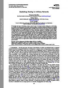
Based on its topology, an interconnection network may be classified as a sharedmedium network, a direct network, an indirect network, or as a hybrid between these classes [43]. In a shared-medium network, the transmission medium is shared by all the terminals. Shared-medium networks have the advantages of potentially low cost and inherent ability to support broadcast communication. Because the bandwidth is shared by all the terminals sharing the medium, however, a pure shared-medium network is only able to support a limited number of terminals. In a direct network on the other hand, a node is connected to each of its neighbouring nodes through separate point-to-point links. A node may relay traffic for other nodes, thereby enabling communication between non-neighbouring nodes through the use of multihop communication. Point-to-point links are also used in indirect networks. In an indirect network, each terminal is connected by a point-to-point link to a switch, which again may be connected to other switches. Networks with mesh and torus topologies, which are the topologies considered in this thesis, are usually considered to be direct networks. The distinction between direct and indirect networks is not always strong, however. For instance, a direct network where each node has an integrated switch module could also be considered as an indirect network where each terminal is connected to a single switch, which again is connected to other switches. Figure 2.1a shows a two-dimensional torus with four nodes in each dimension. As can be seen, each node in a two-dimensional torus is connected to exactly four neighbours. A topology where each node is connected to the same number of neighbours, such as in a torus, is said to be regular [43]. Torus topologies are also often referred to as k-ary n-cubes, where k specifies the number of nodes along each dimension and n the number of dimensions. Thus, the two-dimensional torus topology in Figure 2.1a, with four nodes in each dimension, may be referred to as a 4-ary 2-cube. To avoid the long wraparound links connecting the nodes on the edges, the torus may be folded as shown in Figure 2.1b. Notice that the logical structure of a folded and unfolded torus is the same though. The unfolded version will therefore be used for illustration purposes in this thesis, although the folded version may be preferable for implementation purposes. Figure 2.2a shows a two-dimensional mesh with four nodes in each dimension, also referred to as a 4-ary 2-mesh. As can be seen, a mesh is simply a torus without the wraparound links. Because the wraparound links are missing, the nodes on the edges of the mesh have less links than the inner nodes of the mesh. For both mesh and

CHAPTER 2. INTERCONNECTION NETWORKS

10

(b)

(a) Figure 2.1: (a) A two-dimensional torus (4-ary 2-cube). (b) A folded one-dimensional torus (4-ary 1-cube). torus topologies, higher dimensional networks may be constructed by connecting two or more lower dimensional networks. Figure 2.2b shows a three-dimensional mesh with two nodes in each dimension, that is, a 2-ary 3-mesh, constructed by connecting two 2-ary 2-meshes. Mesh and torus topologies have many similar characteristics, but also important differences. As to the similarities, both mesh and torus topologies are well suited to take advantage of communication locality in parallel applications [3]. Furthermore, both topologies are strictly orthogonal [43]. A strictly orthogonal topology has at least one link in each dimension, and each link is in exactly one dimension. Because it is then possible to traverse any given dimension from any node in the network, routing is simplified and can be implemented in hardware. This is often done in large scale systems, while small and medium size systems usually employ routing tables [93]. For instance, there are no routing tables in the BlueGene/L supercomputer [1], while routing tables are used in the Alpha 21364 [79] and in the Cray T3E [98]. As opposed to the mesh, the torus is also a symmetric topology, meaning that the topology looks the same from every node. This provides for a better load balance and may further simplify routing. We say that a topology is connected if there is at least one path between all the non-faulty nodes in the network. A link or node is redundant if it can be removed and the topology remains connected. Both the torus and the mesh offers redundancy. This is an important feature in our context, as it allows the topology to remain connected even if a link or a node fails. However, even if the topology remains connected, faults alter the characteristics of the topology. For instance, a torus is no longer regular nor symmetric if a link fails. Mesh and in particular torus topologies are often preferred for systems where scalability and redundancy are important design criteria. For instance. in the BlueGene/L [49], 65,536 nodes are connected in a three-dimensional torus topology, clearly

2.1. TOPOLOGIES

11

(b) (a) Figure 2.2: (a) A two-dimensional mesh (4-ary 2-mesh). (b) A three-dimensional mesh (2-ary 3-mesh).

demonstrating the scalability of the torus topology. A three-dimensional torus is also employed by the Cray XT3 and XT4 systems [25]. In the Red Storm [71], 12,960 nodes are connected in a three-dimensional mesh. At the other end of the interconnection network range, two-dimensional mesh and torus topologies are also a popular choice for networks on-chip [123], because they can be easily packaged onto the chip. For instance, in a prototype from Intel [64], 80 cores are connected in a two dimensional mesh on a single processor chip. Torus and mesh topologies are also found in other types of systems. For instance, a threedimensional torus is used to provide an economically scalable switching fabric in the Avici TSR [28] internet router. When deciding between a mesh or torus topology, the offered bandwidth, latency, and cost may be deciding factors. A bisection of a network is a minimal set of links that must be removed in order to divide the network into two halves. The total bandwidth of these links is the bisection bandwidth. With uniform traffic, half the traffic crosses the bisection. Thus, the minimum bisection bandwidth of a network gives a measure of the theoretical capacity of the network. Thus, the fact that a torus provides twice the bisection bandwidth of an equivalent mesh might be a deciding factor. Let us define the distance between two nodes as the minimum hop count between these two nodes. The diameter of a network is then the maximum distance between any two nodes in the network. Because of the wraparound links, a torus has a smaller diameter, and a shorter average distance between the nodes, than a mesh of the same size. On the other hand, a torus has significantly higher wiring costs because of the additional wraparound links. Furthermore, as we will see, in sections 2.3 and 2.4, torus networks also require additional attention in order to avoid deadlocks.

CHAPTER 2. INTERCONNECTION NETWORKS

12

2.2

Flow Control

As mentioned in the introduction to this chapter, the way packets are buffered is determined by the flow control policy. Store-and-forward is maybe the most well known method of flow control,1 due to its use in wide area networks such as the Internet [60]. Using store-and-forward, the entire packet is stored before it is forwarded onto the next hop. As an implication, the buffers must at least be large enough to store an entire packet. Because the entire packet is buffered before it is forwarded, corrupt packets may be discarded. A disadvantage when using this method, however, is that the head of the packet makes no forward progress while waiting for the tail of the packet, thus, a new serialization delay is incurred at each hop. The repeated serialization delay experienced by store-and-forward can be avoided by using wormhole flow control instead.2 With wormhole flow control, each packet is divided into flow control units, called flits for short. The addressing information is contained in the head flit and a switch may forward the head flit once it is received. The channel is then reserved until the tail flit has passed, so that the remaining flits can simply trail after the head flit. Using this method a channel is not strictly required to have buffer capacity for more than a single flit, meaning that the flits of a packet may be spread out across several nodes in the network, like a worm. If contention occurs and the head flit is blocked, waiting for a resource, all the trailing flits are blocked as well. Because the resources held by the trailing flits throughout the network remains unavailable to other packets until they are released by the tail flit, this behavior is susceptible to spread congestion throughout the network. Wormhole flow control has for instance been implemented in the Cray T3D [68] and in Myrinet [11]. Another alternative flow control is virtual cut-through [67]. With virtual cutthrough [67], there must be enough buffer space at each switch to store an entire packet like in store-and-forward. Still, virtual cut-through allows the head of the packet to be forwarded once it is received, like in the case of wormhole flow control. Thus, when there is no contention for resources, virtual cut-through behaves like wormhole flow control, avoiding the repeated serialization delay. When contention occurs, virtual cut-through buffers the packet at the switch like store-and-forward does, preventing a blocked packet from occupying resources at more than one node. Thus, virtual cut-through is able to provide the low latency of wormhole flow control, while at the same time preventing blocked packets from blocking resources throughout the network, at the cost of requiring buffers large enough to store an entire packet. With virtual cut-through (and store-and-forward), the flit size equals the packet size. 1 Some of the methods described in this subsection, that is, store-and-forward, wormhole, and virtual cut-through, are often referred to as switching or routing techniques. Because these methods specify how buffers are allocated to packets, they are referred to as flow control policies in this thesis. This is consistent with [35] and [17]. 2 According to [35], wormhole flow control was first implemented on the Torus Routing Chip [33]. Wormhole flow control is also considered in [34] and [29], which acknowledge wormhole flow control to [100] and [99] respectively.

2.2. FLOW CONTROL

13

Thus, as opposed to wormhole, flow control is conducted on a packet by packet basis. Still, as each flit may be divided into phits (i.e., physical transfer units), a switch may start forwarding the head of the packet once the packet header has been received (granted that there is enough free buffer space at the next hop to store the entire packet). Virtual cut-through is for instance used in the BlueGene/L [1] and in the Alpha 21364 [79]. Because a switch may start forwarding the packet before it is completely received when virtual cut-through is used, it may not be possible to drop a corrupt packet. Still, link level retransmission of corrupt packets can be achieved. In the BlueGene/L [1], for instance, this is achieved by including a valid indicator at the end of each packet. Thus, if the cyclic redundancy check fails, the packet is marked as invalid and a time-out mechanism is used to retransmit the packet. When virtual channels [30] are used, flow control is performed per virtual channel and each virtual channel must therefore have enough buffer space to store at least one flit. Having multiple virtual channels has the advantage that a blocked packet may be bypassed by packets on other virtual channels, much like traffic on a multilane road, thereby reducing head-of-line blocking. The virtual channels, that have a (non-blocked) flit ready to transmit, arbitrate for access to the physical channel. Thus, the physical channel only remains idle if none of the virtual channels are ready to transmit. Multiple virtual channels are particularly beneficial in networks with wormhole flow control. With wormhole flow control, in the absence of virtual channels, a blocked packet would hold all the physical channels between the head and the tail flit idle. When virtual channels are used, only the virtual channels held by the blocked packet remain idle, enabling the other virtual channels to still use the physical channels.

2.2.1

Backpressure

Independent of which of the previously described flow controls that are used, the upstream node needs to know if the downstream node has enough buffer space in order to receive an additional flit. Phrased in another way, the downstream node must provide backpressure preventing the upstream node from transmitting flits when there is not sufficient free buffer space at the downstream node. Having such a backpressure mechanism is essential for providing lossless networks. For the purpose of providing this backpressure, credit-based flow control is typically used when the buffers are only large enough to hold a low number of flits, while on/off flow control is typically used when there is buffer capacity for a large number of flits [35]. If virtual channels are used, backpressure is applied per virtual channel. With credit-based flow control, the upstream node is granted a number of credits corresponding to the buffer space available at the downstream node. The upstream node detracts one credit for each flit transferred. When the downstream node forwards a flit, thereby vacating buffer space for one flit, the credit is increased by one. A credit reaching zero indicates that the buffer at the downstream node is full. In this case the upstream node is not allowed to send another flit before it receives a

CHAPTER 2. INTERCONNECTION NETWORKS

14

(a)

(b)

Figure 2.3: (a) A resource dependency graph for three resources r1 , r2 , and r3 . There is a dependency from r1 to r2 , from r2 to r3 , and from r3 to r1 . (b) A cyclic wait-for graph, representing a deadlocked situation, for three packets (p1 , p2 , and p3 ) holding each their resource and waiting for one of the other packets to release their resource. new credit. Notice that, if the buffers only have capacity for a single flit, the channel remains idle during the time that pass after the flit has been transmitted by the upstream node until a new credit is received from the downstream node, indicating that the flit has been forwarded to the next node. Thus, although buffer capacity for a single flit is sufficient for this method to work, higher buffer capacity is required in order to make full utilization of the channel capacity. Having the downstream node send a credit each time there becomes a new buffer vacancy may generate an unnecessary amount of control traffic when the buffer capacity is large. Using on/off flow control, the receiver is allowed to transmit flits until it receives an off signal from the receiver. After receiving an off signal the sender is not allowed to transfer any more flits to that receiver until it receives an on signal. In order to avoid buffer overflow, the downstream node must send the off signal once the buffers are filled beyond a threshold that takes into account the delay incurred after sending the off signal and until transmission is stopped at the upstream node. As before, buffer capacity should be large enough in order to enable the channel capacity to be fully utilized.

2.3

Dependencies and Deadlock

The fact that packets may block, waiting for a resource (i.e., a buffer/channel) held by another packet, creates dependencies in the network. We say that there is a dependency from a resource ra to a resource rb , if a packet holding ra may wait for rb .3 If there is a dependency from ra to rb and from rb to rc , there is also dependency from ra to rc . Resource dependencies may be depicted in a resource dependency graph, like in Figure 2.3a. Let us consider the scenario in the figure and assume that there are three packets, p1 , p2 , and p3 , that hold each their resource. Packet p1 holds resource 3 When a packet waits for a resource, we assume that the packet will continue to wait until the resource becomes available.

2.3. DEPENDENCIES AND DEADLOCK

15

r1 and waits for resource r2 , packet p2 holds resource r2 and waits for resource r3 , and packet p3 holds resource r3 and waits for resource r1 . In other words, p1 waits for p2 , p2 waits for p3 , and p3 waits for p1 . Because all three packets wait for one of the other packets, to release their resource, no progress can be made. A situation like this is referred to as a deadlock. Such wait-for relationships between packets can be represented in a wait-for graph [24], like in Figure 2.3b. A cycle in the wait-for graph means that there is a deadlock. Once a deadlock has occurred in the network, other packets may deadlock waiting for the resources held by the deadlocked packets. Thus, it is imperative that deadlocks are not allowed to persist in the network. A deadlock can be resolved by breaking the cycle in the wait-for graph. Thus, one can recover from a deadlock by dropping one of the packets creating the cycle. With the Disha deadlock recovery scheme [5], instead of dropping the packet, the packet is routed to the destination using a deadlock-free lane. The deadlock-free lane is enabled by having a single flit buffer at each node dedicated to this purpose. Such deadlock recovery schemes are based on the assumption that deadlocks are relatively rare, which often is the case [89], and also require deadlocks to be detected. Although deadlocks could potentially be detected by analyzing the wait-for graph, a time-out based approach induces less overhead. Although deadlock recovery is a feasible approach, almost all modern interconnection networks are based on deadlock prevention [35], that is, preventing deadlocks from happening in the first place. Thus, in this thesis, we only consider deadlock-free networks. Notice that there can only be a cycle in the wait-for graph if there is also a cycle in the dependency graph. Thus, deadlocks can be avoided by ensuring that there are no cycles in the dependency graph. For a given topology, cyclic dependencies can be removed by restricting the routing function. Given both a topology and a routing function, cycles in the dependency graph can be removed by adding virtual channels [34]. Using these approaches, the channels can be enumerated and given an order in which they are used, thereby ensuring that there are no cycles in the dependency graph. When adaptive routing is used, however, it is possible to have cycles in the dependency graph and for the routing function still to be deadlock-free. It is shown in [37][38][39] that a routing function is deadlock-free if there exists a routing subfunction which is connected and has no cycles in its extended dependency graph. The channels belonging to the deadlock-free routing subfunction are referred to as escape channels, and serve to enable packets to escape from cycles. We refer to the remaining channels as adaptive channels. The extended dependency graph includes direct and indirect dependencies.4 Given two escape channels, c1 and c2 , there is a direct 4

In [38] and [39] the definition of the extended dependency graph also includes cross dependencies. Cross dependencies are introduced when some channels are used both as escape channels and as adaptive channels (i.e., they are used as escape channels for some destinations and as adaptive channels for other destinations). Because routing functions with cross dependencies are not used in this thesis, the extended dependency graph definition from [37] is sufficient for our purpose. According to [35], routing functions with cross dependencies are almost never used in practice.

CHAPTER 2. INTERCONNECTION NETWORKS

16

dependency from c1 to c2 if a packet may request and wait for c2 immediately after it has obtained c1 . If there is an indirect dependency from c1 to c2 , a packet may wait for c2 while still holding c1 followed by some non-escape (i.e., adaptive) channel(s). Notice that indirect dependencies only apply to networks with wormhole flow control where packets may block holding multiple channels at the same time. If there are cycles in the extended dependency graph created by indirect dependencies, these dependencies can be broken by not allowing packets to use an adaptive channel after having used an escape channel. If there are no dependencies in the extended dependency graph, however, packets can switch between escape and adaptive channels at each hop. In the next subsection we will see examples of several routing algorithms for mesh and torus topologies. Dimension-order routing, direction-order routing, and the turn model are all examples of routing algorithms that remove cyclic dependencies by restricting the routing function. Given that such routing algorithms are to be used in torus topologies, virtual channels can be added to remove the cyclic dependencies introduced by the wraparound links. These deadlock-free routing algorithms obtained by restricting the routing function, and potentially adding virtual channels, can again be used as deadlock-free routing subfunctions for adaptive routing algorithms.

2.4

Routing

The path(s) a packet can take through the network is determined by the routing algorithm. Packets that have a single destination are routed according to unicast routing, while packets with more than one destination are routed according to multicast routing. As stated previously, only unicast routing is considered in this thesis. Routing algorithms may be further classified as oblivious or adaptive. An oblivious routing algorithm does not take the state of the network into account, and may be deterministic or non-deterministic. When a deterministic routing algorithm is used, all the packets from a given source to a given destination follow the same path. A non-deterministic oblivious routing algorithm may choose among alternative paths to the same destination without considering the state of the network, for instance by random selection. An adaptive routing algorithm, on the other hand, uses the state of the network to choose among alternative paths to the same destination. Typically, an adaptive routing algorithm estimates congestion based on the local queue lengths and tries to avoid congested links. In order to provide sustained performance under non-uniform loads, many systems such as the BlueGene/L [1], the Alpha 21364 [79], and the Cray T3E [98] use adaptive routing. Adhering to this trend, the fault-tolerant routing algorithms proposed during the work on this thesis also provide support for adaptive routing. Routing algorithms may be either minimal or non-minimal. A minimal routing algorithm only routes packets through minimal paths, while a non-minimal routing algorithm may use non-minimal paths as well. Deterministic routing algorithms are usually minimal, while some non-deterministic (i.e., adaptive or non-deterministic

2.4. ROUTING

17

oblivious) routing algorithms use non-minimal paths in order to try to balance the load in the network. When non-minimal routing is applied, it must be ensured that packets eventually reach their destination. A situation where a packet is being continuously routed around in the network, never reaching its destination, is referred to as a livelock. Although non-minimal paths may help improve load balance, such algorithms also tend to increase latency and consume more network resources [43]. Thus, the solutions for fault-tolerant routing presented in this thesis use minimal routing in the fault-free case. However, non-minimal paths will be used in order to circumvent faulty components. A given routing algorithm may be implemented using source routing or incremental routing. When source routing is used, the complete path is included in the packet header by the source node. When incremental routing is used, on the other hand, the address of the destination is included in the packet header and routing is performed on a hop-by-hop basis. Incremental routing may either be algorithmic or table-based. Because mesh and torus topologies are orthogonal, algorithmic routing can easily be performed based on the offset to the destination in each dimension. Such algorithmic routing is fast and does not require storage space for routing tables, as is the case with table-based routing. On the other hand, the flexibility offered by table-based routing may be beneficial when dealing with faults or incomplete topologies. Furthermore, there exist many methods to reduce the storage space required by routing tables and to optimize their access speeds [20]. As mentioned in Section 2.1, large scale systems often utilize algorithmic routing implemented in hardware, while small and medium size systems often employ routing tables [93]. For instance, routing tables are not used in the BlueGene/L [1], while they are employed in both the Alpha 21364 [79] and the Cray T3E [98]. Considering that the path is determined at the source node when source routing is applied, adaptive routing algorithms are usually employed in combination with incremental routing. Consequently, because the methods presented in this thesis support adaptive routing, they are mainly intended to be used with incremental routing. The remainder of this chapter provides an overview of the routing algorithms that have been used as a basis for the fault-tolerant routing algorithms in this thesis.

2.4.1

Dimension-Order Routing

For mesh and torus topologies, dimension-order routing (also known as e-cube routing) [111] is the most commonly used deterministic routing algorithm. Deterministic routing is simple to implement and enables in order packet delivery, so that packets are not required to be reordered at the destination node. On the downside, deterministic routing algorithms are not able to adapt to different traffic patterns and therefore provides poor worst-case performance. Using dimension-order routing, packets are routed in the order of dimensions. For instance, given a two dimensional mesh network, packets are typically first routed in the X dimension (i.e., the first dimension) and then in the Y dimension (i.e., the second dimension). Because of the way packets

18

CHAPTER 2. INTERCONNECTION NETWORKS

are routed, such dimension-order routing is sometimes referred to as XY-routing. Because packets are routed in the order of dimensions, cyclic dependencies are avoided in meshes. When applying dimension-order routing in torus topologies, the cyclic dependencies may be broken by adding virtual channels [34]. Two virtual channels per physical channel are sufficient to provide deadlock-freedom in n-dimensional torus topologies. When a packet is routed in a given dimension, the packet is routed on the first virtual channel if the coordinate of the destination node is higher than the coordinate of the current node in that given dimension. Otherwise, the packet is routed on the second virtual channel. Although this scheme ensures deadlock-freedom, it results in uneven usage of the virtual channels [2]. A better balance between the virtual channels has been achieved in the Cray T3D [97]. In the T3D, there are two logical datelines in each direction, of each dimension of the network, one for each virtual channel. The datelines are positioned in such a way as to minimize the number of routes that cross them, and the two datelines within the same direction are separated by the maximum distance (i.e., halfway around the ring). Thus, a given packet will at most cross a single dateline in a given dimension/direction. If a packet is to cross a dateline in the dimension/direction it is currently being routed, it is routed on the corresponding virtual channel. The routes that do not cross a dateline, within a dimension, are unconstrained and are used to optimize the virtual channel balance.

2.4.2

Direction-Order Routing

While dimension-order routing restricts routing to a given order of dimensions, directionorder routing ensures deadlock-freedom by restricting routing to a given order of directions. In the Cray T3E [98], direction-order routing is performed according to the following order: X+, Y+, Z+, X-, Y-, and Z-.5 Compared to dimension-order routing, direction-order routing provides for increased routing flexibility and nonminimal paths. Still, the dependency graph is clearly acyclic in mesh networks. By using two virtual channels, direction-order routing can also be made deadlock-free in torus topologies. The Cray T3E applies a single dateline within each ring, and any packet crossing the dateline in a given direction is required to switch from the first to the second virtual channel. Similar to in the Cray T3D, routes that do not cross the dateline within a direction are used to optimize the virtual channel balance in that direction. 5 The Cray T3E use three routing bits in the packet header to indicate the direction a packet is to be routed in each dimension [35]. Thus, a packet can generally only be routed in one direction of a dimension. However, an additional initial hop in a positive direction and a final hop in the Zdirection is also supported, in order to provide fault tolerance and higher system granularity (i.e., by supporting incomplete torus topologies with partial planes).

2.4. ROUTING

2.4.3

19

The Turn Model

Higher adaptivity, than what is provided by direction-order routing, can be provided by using the turn model. The turn model [51] provides deadlock-free and partial adaptive routing, in meshes, by prohibiting the minimal number of turns to avoid cyclic dependencies. There are several ways in which a minimum number of turns can be removed in order to avoid cycles, thus, the turn model provides for several different routing algorithms. For instance, for two-dimensional meshes, the turn model provides the west-first, the north-last, and the negative-first routing algorithms by prohibiting different turns. The west-first routing algorithm prohibits turns to the west,6 and therefore requires packets to be routed west first, if they are to be routed in that direction at all. The north-last algorithm, on the other hand, does not allow a packet that is being routed north to turn in any direction, thereby requiring packets to be routed north last. Finally, negative-first forbids turns from positive (i.e., north/east) to negative directions (i.e., south/west). Positive-first, another variation of the turn model, is an equivalent to negative-first that forbids turns from negative to positive directions. It may be noticed that positive-first allows all the transitions allowed by the direction-order routing used in the Cray T3E (i.e., X+Y+X-Y- when considering only two dimensions), in addition to the north-to-east (i.e., Y+ to X+) and south-to-west (i.e., Y- to X-) transitions. In [12], north-last routing is shown to provide lower throughput than dimensionorder routing under both uniform, local, and hot-spot traffic patterns. However, one should be cautious about drawing general conclusions about the performance of north-last (or the turn model in general) based on these results alone. Dimensionorder routing is known to perform very well under uniform traffic [43], while adaptive routing algorithms have their strength for non-uniform traffic patterns. Considering that the local and hot-spot traffic patterns applied in [12] are basically uniform traffic patterns with some local/hot-spot traffic on top, it could be that these traffic patterns are too uniform to give adaptive routing (i.e., north-last) an edge. This theory is strengthened if we consider the results in [23]. In this paper dimension-order routing is shown to have a higher saturation point than negative-first and west-first under limited hot-spot traffic. However, it is also shown that negative-first and west-first outperforms dimension-order routing when the amount of hot-spot traffic is increased. A thorough analysis of the turn model, under uniform traffic in two-dimensional meshes, is provided in [47]. The relative decrease in performance compared to dimension-order routing is explained by the additional channel dependencies in the turn model. For instance, using dimension-order routing (i.e., XY-routing), an X+ channel may be blocked waiting for a Y-, Y+, or X+ channel and a Y+ channel may only be blocked waiting for another Y+ channel.7 If for instance positive-first is used, on the other hand, both X+ and Y+ channels may be blocked indirectly waiting for 6 The turn model refers to the X- direction as west, the X+ direction as east, the Y+ direction as north, and the Y- direction as south. 7 Blocking may also be caused by blocked terminal (i.e., drain) channels independent of the routing algorithm in use.

20

CHAPTER 2. INTERCONNECTION NETWORKS

X+, Y+, Y-, and X- channels (while X- and Y- channels may be blocked waiting for X- and Y- channels). Thus, positive channels are subject to more blocking than negative channels. This behaviour is likely to be more severe when wormhole flow control is used, since the effect of blocked packets is then aggravated. Thus, it is possible that the performance comparisons with dimension-order routing in [12] (and in [23] for that matter) would have been more favorable for the turn model if virtual cut-through had been applied instead of wormhole flow control.

2.4.4

Adaptive Routing Using Escape Channels

We have seen that direction-order routing and the turn model offers partial adaptivity. As discussed in Section 2.3, fully adaptive routing algorithms can be constructed by relying on deadlock-free escape channels according to the theory proposed by Duato [37][38][39]. When restricted to minimal paths, such routing algorithms are sometimes referred to as Duato’s protocol [43]. We will refer to the set of virtual channels used as escape channels as an escape layer, and the set of virtual channels used as adaptive channels as an adaptive layer. The direction-order routing used in the Cray T3E [98] (discussed in Section 2.4.2) actually serves to provide a deadlock-free escape layer for adaptive routing. At each hop, a packet can either use an adaptive channel or a direction-order escape channel, but a packet is not allowed to block waiting for an adaptive channel. Because virtual cut-through is applied in the T3E, there are no indirect dependencies and it is therefore sufficient that the dependency graph of the escape routing function is free from cyclic dependencies. If wormhole flow control is applied, it must also be verified that the extended dependency graph (i.e., including both direct and indirect dependencies) is free from cyclic dependencies. In that case, it is recommended that minimal routing is used, as very few non-minimal routing functions have an extended channel dependency graph that is free from cycles [43]. Alternatively, packets may be restricted from reentering the adaptive layer after having used an escape channel.

2.4.5

Adaptive Bubble Routing

Adaptive routing is also used in the BlueGene/L [113]. However, in this case, the escape layer is implemented quite differently. Instead of relying on virtual channels, to break the cyclic dependencies introduced by the wraparound links of the torus topology, the bubble flow control [17] is used. Recall, from Section 2.3, that a deadlock is represented by a cycle in the wait-for graph. The bubble flow control avoids deadlocks within a ring by ensuring that there is always a bubble in the wait-for graph, thereby preventing a cycle in the wait-for graph to be completed. A bubble in the wait-for graph can be ensured by only allowing a packet to be injected into the directional ring if there is free buffer space for one more packet after the packet has been injected. Although it would suffice with a single bubble within the ring, it is much simpler from an implementation point of view to just make sure that there is

2.4. ROUTING

21

space for one more packet in the local buffer. Also notice that the bubble flow control is intended to be used in combination with virtual cut-through, as it would be much more complex to ensure that a bubble is present if wormhole flow control was used. An issue with the bubble flow control is that a downstream node could be prevented from injecting packets into the network due to continuous traffic from upstream nodes. When bubble flow control is used as an escape layer for adaptive routing [91], however, this is not an issue as access to the adaptive layer is unrestricted. If bubble flow control is used for deterministic routing, on the other hand, additional injection control mechanisms are required [17].

Chapter 3 Fault Tolerance Fault tolerance is defined as the ability of a system to continue operation despite the presence of faults [83]. In that sense, fault tolerance is closely related to concepts such as reliability, availability, and dependability, as it may serve to provide these features. According to Von Neuman [80], “the basic principle of dealing with malfunctions in nature is to make their effect as unimportant as possible and to apply correctives, if they are necessary at all, at leisure.” This principle is a good example of the desirable behaviour of a fault-tolerant system, that is, minimizing the effects of faults until the faults potentially are corrected. In an interconnection network, bit-errors may occur on transmission links or in memories. Such transient errors may be detected using error control codes, like cyclic redundancy checks, and then be corrected by link-level retransmission or error correction codes. Other failures, such as a broken link-cable or memory-chip, are more permanent in nature. We assume that such permanent failures are detected and contained on a node or link boundary. Thus, faults are assumed to be failstop [95], meaning that we do not consider Byzantine (i.e., malicious) faults [72]. In the context of fault-tolerant routing in interconnection networks, these are common assumptions. Although mechanisms for detecting faulty components are outside the scope of this thesis, the status of a link may be determined by measuring its bit-error rate in addition to using a timeout mechanism. For instance, in the SGI Spider interconnect chip [48], the link is shut down if a packet has not been successfully transmitted after several attempts. Also, because transient-errors affect performance and may indicate a failing component, bit-errors are recorded for each port. Notice that, when such a scheme is used, a faulty node may also be detected as a link failure by each of its connected neighbours. It may be observed, from the previous discussion, that transient and permanent faults are not completely disjoint. Specifically, a link with frequent transient errors may be considered to have a permanent failure. Furthermore, a permanent failure may disappear if the faulty component is repaired or replaced. Nevertheless, the distinction between transient and permanent failures is clearly a useful one. In particular, permanent link and node failures are handled very differently from typical 23

24

CHAPTER 3. FAULT TOLERANCE

transient failures. Permanent faults manifest themselves at the network level as link or node failures. In the case that a fault-tolerant routing algorithm is used, such faults can be circumvented using alternative paths. Because additional load is then placed on the remaining links, some degradation in the network performance must be expected. Thus, when using this strategy, the goal is to provide a graceful performance degradation in the presence of faults. The effectiveness of applying fault-tolerant routing can not be determined by considering the routing algorithm in isolation however. Its effectiveness clearly also depends on other factors such as the topology of the system, the mean time between failures, the mean time to repair, and the requirements of the application(s). Obviously, fault-tolerant routing is limited by the redundancy offered by the topology. Fortunately, both mesh and torus topologies offers redundancy. Even the least redundant of these topologies, the two-dimensional mesh, remains connected in the event that any single node or link is removed. Although removing two random links/nodes could potentially disconnect a two-dimensional mesh, it is much more likely that the network remains connected for all but the smallest networks. For torus and higher dimensional topologies, the offered redundancy is even higher (e.g., one can remove any two links in a three-dimensional mesh, any three links in a twodimensional torus, and any five links in a three-dimensional torus). Furthermore, even if some nodes become physically disconnected, fault-tolerant routing may enable the remaining system to be kept operational. Given that the topology offers sufficient redundancy, fault-tolerant routing may still not provide a satisfactory solution in a system where any degradation in network performance, or loss of processing power, is prohibited. In many practical scenarios, however, a temporary degradation in network performance or processing power is acceptable. Furthermore, when designing a system, the interconnection network is usually not planned to continuously operate at its saturation point. Thus, a small reduction in the peak performance of the network is not necessarily equally reflected in the performance of the application(s). Also, if the mean time between failures is longer than the mean time to repair, the number of simultaneously faulty components is likely to be limited. Thus, given that the provided graceful performance degradation is acceptable, fault-tolerant routing is a viable option for many systems. Even in systems where repairs are not performed/possible, fault-tolerant routing could be an alternative if the performance degradation is acceptable, taking into account the reliability of the individual components over the expected lifetime of the system. In the next section, we will consider what alternatives exist, besides fault-tolerant routing, that can be used to provide a reliable interconnection network. Then, in Section 3.2, fault models pertained to fault-tolerant routing are presented, before we provide an overview of existing fault-tolerant routing algorithms in Section 3.3.

3.1. ALTERNATIVES TO FAULT-TOLERANT ROUTING

3.1

25

Alternatives to Fault-Tolerant Routing

If reliability is to be provided, the alternative to fault tolerance is fault avoidance [7]. Fault avoidance requires each component to have a very high reliability and to be perfectly assembled. Such high quality requirements may significantly increase the cost of a system. Furthermore, as the number of components increase, even a system built from extremely reliable components may not be able to provide sufficient reliability through fault avoidance. Let us for illustration consider a system like the BlueGene/L, with 65,536 nodes and a desired mean time between failures of at least 10 days [113]. If we model all faults as node failures and somewhat simplified assume that the probability of failure is equal, independent, and constant for all the nodes during the lifetime of the system, each node would be required to have a mean time between failures of about 1794 years in order to provide the desired reliability for the entire system.1 What is more, even a system built from extremely reliable components may not be protected against human errors, such as unplugging the wrong cable, and other external factors. Relying solely on fault avoidance also has the disadvantage that the entire system fails completely, potentially without any warning, once the first component fails. Hence, fault avoidance alone is not a trustworthy solution for critical systems where for instance lives are at risk. For non-critical systems, a low mean time to repair, potentially combined with fault avoidance, may provide an alternative to fault tolerance. A disadvantage with this approach, however, is that there is a trade-off between the mean time to repair and the costs of having maintenance personnel and spare parts available. Thus, if the money potentially saved by not investing in a faulttolerant system is not to be eaten up by increased operational costs, one may end up with significant downtime for the system. Although such system downtime may be acceptable in some environments, decreased utilization may reduce the return on investment. Fault tolerance has the advantage of enabling the system to remain operational despite the presence of faults, thereby offering flexibility in when repairs are to be carried out and reducing system downtime. This way, fault tolerance can reduce maintenance costs and potentially increase the return on investment. Furthermore, fault tolerance may reduce the initial system cost for some systems, by lowering the reliability requirements for individual components to the level provided by standard components. Finally, fault tolerance may significantly improve the reliability of a system. In particular, by combining fault tolerance with fault avoidance, highly reliable and scalable systems can be provided. One way to provide fault tolerance is through the use of replicated components. Using this method, the failed component is replaced by its redundant copy in the case of failure. In order for this strategy to be effective, the redundant copies should fail independently from the primary components. As long as the redundancy is not 1 The required mean time between failures of each node (M T BF n), depending on the desired mean time between failures of the entire system (M T BF s), is then given by: M T BF n = M T BF s× number of nodes = 10days × 65, 536 ≈ 1794years.

CHAPTER 3. FAULT TOLERANCE

26

exhausted, redundant components has the advantage of maintaining full performance even in the presence of faults (assuming that the redundant copies are identical to the originals). Redundant components may add significant to the cost of a system, however, and there is also a risk that the hardware used for switching in the redundant copies might fail. If size, weight, or packaging restrictions apply, redundant components may also be undesirable from that point of view. From a routing perspective, a faulty link or node can obviously not be used for forwarding packets. If the routing algorithm in use is not fault-tolerant, a faulty component would typically result in the packets that were to use it being blocked or dropped. In case the packets were blocked, chains of blocked packets would rapidly be created effectively bringing the network to a halt. The alternative, extensive packet dropping, is not much more desirable in a lossless network. A better approach, in the absence of fault-tolerant routing, is to disable a sufficient number of nodes or partition the network in such a way that the faulty component is no longer required. However, such an approach can easily disable a high number of nodes. Even if all the healthy nodes can be partitioned into two smaller networks, such a reduced system might not be able to satisfy the requirements of the application(s), thereby becoming practically useless. Another approach is to bypass the faulty components, potentially together with some healthy nodes as well. For instance, in the BlueGene/L [49], each 512-node midplane can be powered down separately. By having the link-chips on a separate power domain, this can be done without affecting the other planes. Furthermore, to ensure system availability, the entire machine can also be partitioned into segments of eight nodes along any dimension, with each partition remaining a torus.2 Clearly, fault tolerance is a great advantage in many systems, and a necessity for some. By using fault-tolerant routing instead of the previous schemes, fault tolerance can be provided (without requiring spare components) by utilizing the inherent redundancy offered by the topology. Although fault-tolerant routing is likely to incur some performance loss in the presence of faults, fault-tolerant routing comes at a much lower cost than component replication. Furthermore, as opposed to the other fault tolerance schemes not using spare components, fault-tolerant routing may avoid disabling a high number of healthy nodes and partitioning the network.

3.2

Fault Models

In this section we consider fault models related to fault-tolerant routing. More specifically, the implications of using a static or dynamic fault model are discussed in Section 3.2.1. Then, in Section 3.2.2, we describe different extents to which fault information can be made available. Finally, in Section 3.2.3, we present fault models for specifying 2 The BlueGene/L is also able to provide some fault tolerance by injecting packets in a manner that forces them to take non-minimal paths avoiding the faults. This mechanism is able to tolerate up to three faults, in a partition, provided that they are not collinear. However, due to software and performance impacts, this mechanism is not intended for use with general applications.

3.2. FAULT MODELS

27

the combinations of faults supported by a fault-tolerant routing algorithm.

3.2.1

Static or Dynamic

Faults in an interconnection network can be dealt with statically or dynamically. When a static fault model is used, all the faults need to be known when the system is started. Thus, when a fault occurs, the system has to be restarted in order to continue operating. Considering that a system’s mean time between failures may be lower than the execution time of some of its hosted applications [93], this method may need to be combined with a rollback-recovery mechanism such as checkpointing in order to be effective.3 If restarting the system when faults occur is not desirable, either because of the overhead imposed by relying on a recovery mechanism (e.g., maintaining checkpoints and rolling back to the last checkpoint at system failure/restart) or because continued operation is required, a dynamic fault model should be used. When a dynamic fault model is used, the system remains operational while measures are taken to circumvent the faulty component(s). A dynamic fault model has some complicating implications though. For instance, a packet that is being transmitted across a failing link may be split in two. In the case that virtual cut-through (or store-and-forward) is used, it is feasible to have the upstream node to retransmit/reroute the packet onto another link. However, this can not be done when wormhole flow control is used. In that case, the flits that have already been transmitted over the faulty link, including the packet header, are no longer available to the upstream node. The Reliable router [32] handles this by storing the header-flit of the packet until the channel for that packet has been released. As a result, the router on the downstream side of the failing link can append a tailflit to the received flits, while the upstream router can append a new header to the remaining flits, based on the stored header, and forward them onto another link. At the destination node the fragmented packet can then be reassembled, discarding any duplicate flits. In the case of a router failure, things become even more complicated if one is to ensure that no packet loss is to occur in the network. Again, in the Reliable router, this is solved by requiring that all flits are buffered at two different routers at all times. Thus, when node 1 forwards a flit to node 2, node 1 continues to buffer the flit until node 2 confirms that the flit has been successfully forwarded to node 3. This way, node 1 is able to retransmit the flit in case node 2 fails before the flit has been successfully forwarded to node 3. The advantage of using such a method is that the network remains lossless even in the case of single node failures, and therefore may not require an end-to-end retransmission scheme to be in place. On the other hand, such a scheme increases the buffer requirements at the routers and complicates the flow control. An alternative strategy for dealing with link and node failures under a dynamic fault model is to accept that some packets may be lost when a component fails. The 3

A survey of rollback-recovery protocols can be found in [44].

CHAPTER 3. FAULT TOLERANCE

28

node on the downstream side of a failing link must still ensure that any channels that have been reserved downstream are released, by inserting a tail flit (marking the packet as invalid), but otherwise fragments from cut-off packets can simply be dropped. Likewise, it is then also accepted that the packets buffered at a router is lost if that router fails. Using this strategy assumes that end-to-end reliability is provided by other means, or that the applications are able to deal with packet loss. End-toend reliability can for instance be achieved through the use of a reliable transmission protocol. The Reliable Message Passing Protocol [94] is one such protocol, targeted specifically at high-speed networks where errors are rare. Furthermore, end-to-end reliability is provided by some current message passing interface (MPI) implementations, such as LA-MPI [6], and is also to be supported in future Open MPI [90][124] implementations. Another issue, when a dynamic fault model is used, is that of ghost dependencies [85]. When dynamically changing the routing function, there are likely to be packets in the network that have been routed according to the old routing function. After changing the routing function, these packets may occupy channels on which they are not allowed to be routed according to the new routing function, thereby introducing ghost dependencies. Although both the old and the new routing functions are deadlock-free, the additional ghost dependencies may potentially lead to deadlock. Thus, ghost dependencies must be taken into consideration when determining if a dynamic fault-tolerant routing algorithm is deadlock-free or not.4 In the case that cyclic dependencies are created, the ghost dependencies may be removed by having the packets absorbed by the node, to be reinjected later, or dropped. Notice that because the old routing function will often be disconnected (i.e., when a fault has occurred), packets may be prevented from being routed to their destination using the old routing function. As we have seen, a dynamic fault model has both advantages and disadvantages compared to a static fault model. The main advantage is that it enables the system to remain continuously operational even when network components fail. On the other hand, the use of a dynamic fault model incurs additional complexity. Although a static fault model may require the use of a rollback-recovery mechanism, such a mechanism may potentially be required in the first place anyway. This is because rollback-recovery may also be used as a precaution against loss of work due to other reasons, such as a terminal failing, an application crashing, or external factors such as a power outage. In the case that a node fails, the applications that were running on that terminal may need to be moved to another terminal. For instance, in the BlueGene/L [49], the primary strategy is to restart the application from a checkpoint on a set of midplanes that does not contain the faulty node. Such high level fault tolerance mechanisms are outside the scope of this thesis however. Anyway, as the choice between a dynamic or static fault model depends on the application requirements, we address fault-tolerant routing under both static and dynamic fault models in this thesis. 4

Further discussion on deadlocks during dynamic network reconfiguration can be found in [42].

3.2. FAULT MODELS

3.2.2

29

Fault Status Information

Fault status information may be distributed through control messages, using the primary network or a separate control network. Apart from the additional cost, a separate control network has the disadvantage that it may also be subject to failures. In the Cray T3E [98], there is a separate virtual network (i.e., virtual layer) used for system initialization and diagnostics. Lossless flow control is not employed in this virtual network (i.e., contention for resources is solved by dropping packets), thereby preventing deadlocks. Because such a virtual network is not subject to deadlocks, it provides high routing flexibility that can be used to circumvent faults. Whether such a separate virtual network is used or not, it is imperative that control messages used for distributing status information can not be blocked directly or indirectly waiting for a faulty component. Fault status information may be collected and distributed using a centralized or a distributed approach. If a centralized approach is used, a central manager has knowledge of all the faults in the network. The central manager may then compute the required changes in the routing function and distribute these to each node. Alternatively, the central manager may distribute the fault status information to all the nodes so that they can act upon this information themselves. By having multiple redundant central managers (or potentially by electing a central manager in some distributed fashion) it can be avoided that the central manager becomes a single point of failure. A distributed approach to fault-tolerant routing, where rerouting decision are taken locally at the node without relying on a central manager for providing fault status information, may depend on varying degrees of fault status information. For instance, some algorithms require global knowledge of faults, while others only require to know the status of its neighbours. Furthermore, some algorithms do not require explicit knowledge of the faults at all, as routing information is distributed instead. This is for instance the case for Up*/Down* routing [96], where the routing function is established by applying a distributed spanning tree algorithm. For such routing algorithms, the non-faulty paths are the information of interest, not the location of the faults. Assuming that fault status information is utilized, k-neighbourhood diagnosis [10] implies that each node has information about the faults within distance k. If k equals the network diameter, global fault status information is used. If k = 1, on the other hand, each node only has knowledge about the status of its immediate neighbours. A relaxation of k-neighbourhood diagnosis is provided by k-reachability diagnosis [10], in which case each node only has knowledge of the faults that are reachable by a non-faulty path of length k or less. Although k-neighbourhood diagnosis is not really achievable if the network has become partitioned, unless a separate control network is used, partitions may be considered to be separate networks. Thus, for practical purposes, the main difference between k-neighbourhood and k-reachability diagnosis is that k-reachability diagnosis requires less fault status information to be distributed, and thereby also provides less information to the nodes. For instance, if

CHAPTER 3. FAULT TOLERANCE

30

1-neighbourhood diagnosis is used, two nodes connected by a faulty link are both to know the status of the other node. If 1-reachability diagnosis is used on the other hand, the status of the other node is unknown to each of the two nodes. The amount of diagnostic information made available to each node is a trade-off between the cost and time to distribute the information (and also the storage space needed to store it) and the optimality of the routing decisions that can be taken based on the information. When global information is available, optimal routing decisions can be made, while access to only local information may result in non-optimal routes. The use of a static fault model facilitates the use of global fault information. When a dynamic fault model is used, on the other hand, a more limited distribution of status information may be preferable in order to reduce the additional complexity, delay, and resource usage incurred by maintaining correct fault status information. A node may maintain fault status information by keeping a list of the known faults and their location. Assuming that the number of faults in the network is limited, such a list requires little storage space. As long as the list of faults is only used for recalculating the routing table when changes occur, the time to access and process the list of faults does not impact network performance (except from potentially when routing tables are being recalculated). In a system without routing tables, however, alternative fault status representations may be preferable. An alternative to keeping a list of all the known faults is to maintain the safety level [125][126] of each node. Given a node with safety level k, there is at least one minimal path from this node to any node within distance k. The safety level concept can be seen as an extension of that of unsafe nodes [73]. An unsafe node is a node which has at least two faulty or unsafe immediate neighbours. The idea behind unsafe nodes is that routing packets through such nodes may cause the packet to be trapped or deviated. Therefore, safe nodes are preferred when making routing decisions.

3.2.3

Faults Tolerated

Different fault-tolerant routing algorithms provide various degrees of fault tolerance, from only tolerating single link or node failures to tolerating any combination of faults as long as the physical network remains connected. More specifically, a routing algorithm is considered to tolerate a given combination of faults as long as it provides a valid route between all the (non-faulty) nodes that are physically connected. Faults may be modeled as node and/or link faults. If a node fault model is used, link faults are treated as node faults. Similarly, under a link fault model, a node fault may be modeled as the failure of all the links of the node. When faults are modeled as individual link or node faults, we say that a routing algorithm is f -fault-tolerant if it is able to tolerate all combinations of f faults (link or node), but there is at least one combination of f +1 faults that is not tolerated. In this thesis, as in most of the literature, link failures are assumed to be bidirectional and we do not address the failure of individual virtual channels (i.e., the entire link is considered to be faulty if

3.2. FAULT MODELS

31

Figure 3.1: Three block (i.e., convex) faults. The bold links and nodes constitute two overlapping f-rings, while the dotted links and nodes create an f-chain.

a virtual channel fails).5 To simplify routing, closely located faults may be combined into fault regions. The shapes of such fault regions are often restricted by the fault model in use. Furthermore, the fault model may impose additional restrictions on the locations of the faults. For instance, faults may not be allowed on the edges of the mesh and there may be a minimum distance between separate fault regions. A routing algorithm applying such a fault model is generally to tolerate all fault combinations conforming to the fault model, thus, the provided fault tolerance is defined by the fault model. In the case that a fault combination is not conforming to the fault model in use, healthy nodes are marked as faulty (i.e., disabled) in order to create proper fault regions. Although healthy nodes are disabled, a fault combination is considered to be tolerated as long as all the nodes, that are neither faulty nor disabled, are connected through valid paths. The simplest fault model in mesh and torus topologies is the block fault model (also referred to as the convex fault model). Under the block fault model, all fault regions are required to have a rectangular shape in a two-dimensional mesh/torus, and a cuboid shape in a three dimensional mesh/torus. Block faults can be created by marking a node faulty if it has a faulty neighbour/channel in at least two dimensions [22]. Three block faults are shown in Figure 3.1. The non-faulty nodes and links circumventing a fault region, marked in bold in the figure, creates an f-ring (i.e., fault-ring) [13]. There can be one f-ring for each fault region, and the nodes/links on 5 From a theoretical point of view, fault tolerance at the granularity of unidirectional virtual channels is achievable in many cases. For instance, a routing algorithm according to Duato’s protocol (discussed in Section 2.4.4) would be able to tolerate the failure of individual adaptive channels, as long as the escape channels remain non-faulty.

32

CHAPTER 3. FAULT TOLERANCE

Figure 3.2: This is the same fault-scenario as in the previous figure, but using a nonoverlapping block (i.e., convex) fault model and assuming that faults on the edges are not supported. The bold links and nodes constitute an f-ring.

the f-ring may be used for rerouting packets around the fault region. If a fault region includes nodes on the border of the mesh, however, an f-ring can not be created. Instead, an f-chain [13] is created, as illustrated by the dotted nodes and links in Figure 3.1. Two f-rings/chains overlap if they have at least one link in common [13], thus, two f-rings/chains may have a node in common without overlapping. A routing algorithm allowing f-rings/chains to overlap, is often said to tolerate overlapping fault regions. In fact, an overlapping block fault model is used in Figure 3.1, as the two f-rings overlap. The main reason why some fault-tolerant routing algorithms do not allow overlapping fault regions is that they impose restrictions on how the virtual channels within the f-rings/chains are to be used, and when f-rings/chains overlap these requirements can not be met without requiring additional virtual channels. The same fault scenario is shown under a non-overlapping block fault model in Figure 3.2. As can be seen, additional nodes must be marked as faulty in order to avoid overlapping f-rings. More specifically, nodes with faulty (or disabled) links/neighbours in both directions of a dimension are part of two f-rings [19], and are therefore marked as faulty. In the scenario in Figure 3.2, we have also assumed that faults on the edges of the mesh are not supported, thus, all the nodes in the rightmost column have been disabled due to the single fault. A stricter version of the block fault model, is to require all fault regions to be square [74] (or cubic in a three dimensional network). Because a node with at most one faulty or disabled neighbour is not able to determine whether it is part of such a region solely based on the status of its neighbours, such fault regions are more complex to construct and maintain than pure block faults if used with a dynamic

3.2. FAULT MODELS

33

Figure 3.3: A fault region under the solid fault model. The bold nodes and links constitute the f-ring.

fault model.6 Furthermore, such a fault model is likely to require more nodes to be disabled. The experimental results in [74] give some indications on the percentage of healthy nodes that are disabled in a 10×10 mesh when using square fault regions. In particular, when 10% of the nodes are faulty, on average less than 12% percent of the non-faulty nodes are marked as faulty, and the entire network becomes disabled when about 20% of the nodes are faulty. Although it may appear that such a method is able to tolerate almost 20% of the nodes being faulty, it is not likely that the system is able to perform satisfactory with such a high proportion of the nodes disabled. In order to reduce the number of disabled healthy nodes, nonconvex fault regions may be used. The simplest of these is the solid fault model. The solid fault model [19] includes all block/convex faults, in addition to all other non-concave fault regions. That is, given a single dimensional section of a solid fault region, there should be no non-faulty node/link between two faulty nodes/links. Any such healthy nodes are marked faulty. A solid fault region is shown in Figure 3.3. As can be seen, a node is disabled because it would otherwise create a gap between the nodes on its right and left sides. If such gaps are to be allowed, concave (i.e., non-solid) fault regions must be supported. By not requiring the nodes within such gaps to be disabled, fault-tolerant routing methods supporting concave faults (as shown in Figure 3.4) are able to tolerate a wide range of faults without disabling healthy nodes. Specifically, such routing algorithms provide additional support for nonconvex faults compared to the solid fault model by also tolerating concave fault regions. Still, such methods may not be able to tolerate arbitrary fault-patterns, and may put some restrictions on the shape of the concavities. Unfortunately, the terms convex, nonconvex, and concave fault regions are not 6

A static fault model is assumed in [74].

34

CHAPTER 3. FAULT TOLERANCE

Figure 3.4: A concave fault region.

consistently used in the literature, as they are sometimes interchanged. In this thesis, however, we will use the definitions that have been provided in this section. Furthermore, although fault regions are most commonly applied to node faults, they are also applicable to link faults.

3.3

Fault-Tolerant Routing Algorithms

In this section we provide a brief survey of fault-tolerant routing algorithms that have been proposed for mesh and torus topologies. The survey is by no means exhaustive, but serves to provide a general overview of different approaches. We only discuss routing algorithms that are targeted at networks with lossless flow control, that is, routing algorithms that take deadlocks into account. Furthermore, only unicast routing is considered in this thesis.7 Notice that if fault-tolerant unicast routing is in place, fault-tolerant multicast/broadcast operations can be implemented in software using unicast, although the performance may suffer compared to when more native support is provided. In order to improve the readability of this section, the fault-tolerant routing algorithms have been divided into different categories that are covered in separate sections. Notice that this classification is mainly performed for readability purposes though. Some of the fault-tolerant routing algorithms only have minor similarities with the other algorithms within their placed category, while others have strong similarities to routing algorithms within several categories. It should also be pointed out that chapters 4 and 5 provide separate discussions about the work most closely related to the methods presented in those respective chapters. 7 Proposals for fault-tolerant multicast in torus and mesh topologies can be found in [75][118][122][65], and fault-tolerant broadcast algorithms in [86][121][66].

3.3. FAULT-TOLERANT ROUTING ALGORITHMS

3.3.1

35

Fault Tolerance through Adaptive Routing

Traditional routing algorithms like dimension-order routing are not able to utilize the redundancy provided by the network topology. Much work has therefore been done to create fault-tolerant routing algorithms that take better advantage of the redundancy offered by the topology. One approach has been to develop adaptive routing algorithms, where the adaptivity can be used to circumvent faulty components. Notice that adaptive routing algorithms are not necessarily fault-tolerant though. A strictly minimal adaptive routing algorithm is not able to handle a single fault, as for instance the source-destination pairs connected by a single minimal path are disconnected by any fault on the minimal path. Linder and Harden [76] proposed a method providing sufficient adaptivity to tolerate at least one fault. However, the number of virtual channels required by their method increases exponentially with the number of dimensions. Chien and Kim [22] observed that the potentially large number of virtual channels required by Linder and Harden is due to the freedom to traverse dimensions in arbitrary order. They therefore proposed planar adaptive routing [22], where adaptivity is limited to adaptive routing in two dimensions at a time. This method requires at most three virtual channels to handle block faults in meshes of any dimension (two virtual channels are sufficient in two dimensional meshes), but does not properly handle faults on the edges of the network. Dally and Aoki [31] proposed adaptive routing using dimension reversals. A dimension reversal (DR) number is associated with each packet, and this number is increased when making a transition to a lower dimension. Deadlock-freedom can then be provided either by requiring that packets with different DR numbers use different virtual layers, or by prohibiting a packet to wait for a channel held by a packet with a lower DR number. Independent of which of the two strategies are used, a packet reverts to dimension-order routing (in the latter case in a separate virtual layer) if the applicable condition does not hold. Thus, if routing adaptivity is used to avoid congestion, the method does not guarantee tolerating a single fault. However, if dimension reversals are only performed to reroute around faults, not to avoid congestion, the number of tolerated faults is proportional to the number of additional virtual layers.

3.3.2

Turn Model Based

We saw in the previous section that the partial adaptivity of planar adaptive routing can be used to provide fault tolerance. As described in Section 2.4.3, partial adaptivity is also provided by the turn model. Glass and Ni [52] used the partial adaptivity provided by the turn model (i.e., negative-first routing) to develop a dynamic fault-tolerant routing algorithm for meshes. The method does not require any virtual channels, but only tolerates n − 1 faults in an n-dimensional mesh. Packets are routed in such a way that there is always enough routing flexibility to circumvent n − 1 faults. This includes routing packets an extra hop during the negative

36

CHAPTER 3. FAULT TOLERANCE

phase in order to provide sufficient flexibility in the positive phase, thus, routing is non-minimal even in the fault-free case. Cunningham and Avresky [27] combine two different variations of the turn model (i.e., north-last and south-last) to provide fault-tolerant routing in two dimensional meshes. One virtual layer is used for north-last routing and another one for southlast routing. Combining north-last and south-last offers increased routing flexibility that can be used to avoid congestion, thereby providing a better network balance. Once a fault is detected, however, adaptive routing is turned off and the routing flexibility is reserved to reroute packets around the fault(s). Because adaptive routing is disabled in the entire network, a single fault inflicts a significant performance loss. Furthermore, although N − 1 faults are tolerated in an N ×N mesh, a high number of healthy nodes may be marked as faulty in order to ensure that the provided routing flexibility is sufficient to keep the remaining nodes connected. A similar method is obtained by Duato in [40], where he proposes a methodology to design deadlock-free fault-tolerant routing algorithms. By applying the methodology to two-dimensional meshes, and combining the west-last and east-last variations of the turn model, a fault-tolerant routing algorithm using four virtual layers is obtained. The resulting routing algorithm is guaranteed to tolerate one single fault without disabling healthy nodes, or alternatively any combination of block faults. Skeie [107] uses the positive-first variation of the turn model to provide partial adaptive fault-tolerant routing in meshes. The method does not require any virtual channels and is based on locally rerouting around faults. In general, rerouting is achieved by using the routing flexibility provided by positive-first routing in combination with altering the routing tables so that packets do not end up in a situation where they would require the use of an illegal turn. In order to distribute rerouting information, separate control lines are used. Although many different fault combinations are tolerated without disabling healthy nodes, there are some combinations of two faults (in a two-dimensional mesh) that are not tolerated. Libeskind-Hadas and Brandt [74] proposed origin-based fault-tolerant routing for meshes without using virtual channels. In origin-based routing, the channels are divided into two classes, IN and OUT channels. The IN channels are used for routing towards the origin, while the OUT channels are used for routing away from the origin. By routing packets in two phases, first towards the origin and then away from the origin, deadlock-freedom is ensured. The positioning of the origin is a tradeoff between the provided routing adaptivity and the origin becoming a bottleneck. Positioning the origin in the negative corner results in negative-first routing and minimizes the bottleneck effect for uniform traffic patterns. Thus, although originbased routing is not based on the turn model, the resulting routing is similar. With origin-based routing, static fault tolerance is provided using square fault regions. In its basic fault-tolerant version, the origin is positioned in a fault-free row and column. All nodes not in the same row/column as the origin have two alternative links to forward packets towards the origin. Because a node with two faulty neighbours would be included in a fault region, this ensures that the origin is reachable from all

3.3. FAULT-TOLERANT ROUTING ALGORITHMS

37

unmarked nodes. When reaching the origin in one dimension, packets are routed to a safe node that is known to have a fault-free path to the destination.

3.3.3

Fault Regions

Boppana and Chalasani [13] proposed a method to tolerate block faults in two dimensional meshes (with dimension-order routing). This method is able to tolerate overlapping f-rings/chains when using four virtual channels and non-overlapping frings when using two virtual channels. In the latter case, f-chains are not used, meaning faults on the edges of the mesh are not supported. Packets are classified by the direction they would be routed in the fault-free case, and the routing in the f-rings/chains is organized so that the different classes use disjoint sets of virtual channels. By combining it with planar adaptive routing [22], the authors also apply the method to higher dimensional meshes. Sui and Wang [110] later showed that the method of Boppana and Chalasani can be improved to only require three, instead of four, virtual channels in order to tolerate overlapping block faults in meshes (while still supporting faults on the edges of the mesh). Similarly, fault regions are also used by Boura and Das [15], who provides support for fully adaptive fault-tolerant routing in n-dimensional meshes using three virtual channels. This method is based on an adaptive routing algorithm previously proposed by the same authors [14]. Because rectangular fault regions are used, they also mark healthy nodes as faulty in order to establish fault regions. However, their method also have a reactivation mechanism, enabling some nodes that have been marked as faulty to be reactivated (for sending and receiving packets, but not for routing) if they are directly connected to a node outside the fault region. Su and Shin [108] proposed another adaptive fault-tolerant routing algorithm for meshes, only requiring two virtual channels. One layer is used for deterministic deadlock-free routing while the other is used for fully adaptive routing, like in the adaptive routing proposed by Duato [37]. In the case of failures, block faults are formed and the fully adaptive channels enclosing the region are turned into deterministic ones that are used for rerouting packets around the region. Because these channels can only be used for rerouting around a single region, only non-overlapping fault regions are allowed. Like in the paper by Boura and Das [15], some nodes within a fault region may still remain active. However, such nodes are required to be directly connected to two nodes outside the fault-region (in each two-dimensional plane). Chalasani and Boppana [19] extended their method to support solid fault regions using four virtual channels. On the other hand, this new method does not support overlapping f-rings or faults on the edges of the mesh. Such support is provided by Kim and Han [70], however, still using the same number of virtual channels (i.e., four). Chen and Chiu [21] later managed to reduce the number of virtual channels to three, still tolerating overlapping solid faults and faults on the edges. More recently, Youn [129] proposed a method only requiring two virtual channels, supporting nonoverlapping solid faults and faults on the edges. Wu [127] proposed a fault-tolerant routing algorithm, for two-dimensional meshes,

CHAPTER 3. FAULT TOLERANCE

38

based on the odd-even turn model [23]. The method does not require any virtual channels and is able to tolerate a type of solid fault regions. However, faults are not allowed at or close to the edges of the mesh and nodes on an f-ring (i.e., nodes on the boundary of a fault region) are not allowed to a be destination nodes. Also, routing is non-minimal in the fault-free case. Although the restrictions can be removed, this requires the addition of virtual channels. Gu et al. [57] have proposed an extension for handling concave fault regions, that can be used with existing proposals for nonconvex faults. However, this extension requires ejecting and reinserting packets when entering and leaving a concave section, thereby increasing the latency and occupying memory at the nodes. Park et al. [87] handle simple concave, non-overlapping, fault-regions in meshes without ejecting/reinserting packets, requiring three or four virtual channels depending on the provided fault tolerance. However, this method does not handle faults on the edges of the mesh. Chalasani and Boppana [18] also proposed a variation of their method for torus, requiring a total of six virtual channels to tolerate non-overlapping block faults. Shih [103] later improved on this by proposing a method tolerating solid faults while maintaining the number of virtual channels. This result was further improved by the same author, proposing a method tolerating overlapping block faults in tori using three virtual channels [104] and another method [105] tolerating overlapping solid faults using four virtual channels. Although not based on fault-regions, Ho and Stockmeyer [61] proposed a method for meshes based on disabling a set of nodes, referred to as lamb nodes, so that the remainder of nodes can communicate using at most two rounds of dimension-order routing. Although the lamb nodes can not be used for processing, they are still used for routing. Furthermore, in order to prevent deadlock, different virtual channels are used for each of the two rounds of routing.

3.3.4

Search Based

Gaughan and Yalamanchili [50] proposed pipelined circuit switching (PCS), where the header sets up a path of virtual channels before the data is sent. PCS provides fault tolerance through the use of misrouting and by allowing the header to backtrack, effectively performing a dept-first search for a valid path. This method is powerful in terms of fault tolerance, but the path setup increases latency even in the fault-free case, especially for small packet sizes and larger networks. In the simulations PCS performed poorly when used with only one virtual channel. The authors account this to the cost of misrouting, but the poor performance may potentially also be explained by the fact that virtual channels are held for an extended period of time due to the setup phase, which again may result in misrouting of other packets. Scouting is a variation of this scheme, proposed by Duato et al. [41]. Using scouting, one does not wait until the entire path is established before sending the data. Instead, the data follows the header at a given distance, allowing the header to backtrack a given number of hops. Although this reduces the latency overhead, it

3.3. FAULT-TOLERANT ROUTING ALGORITHMS

39

still introduces additional overhead and causes channels to be held for a prolonged time. A further improvement is proposed by Dao et al. [36]. In this latter proposal, a configurable flow control is used, enabling a wormhole like flow control to be used in the fault-free case while scouting is used when faults are present. Kim et al. [69] proposed compressionless routing for wormhole routed k-ary ncubes, providing adaptive routing without the use of virtual channels. By ensuring that packets are long enough, so that the first flit is received at the destination before the last flit leaves the source, the sender can verify that the packet is not deadlocked. If a new flit can not be injected for a specified time period, the path held by the already transmitted flits is released using a kill signal and the packet is retransmitted. Like with pipelined circuit switching there may be a significant overhead for short packets in large networks because packets need to be padded if they are not long enough. In the fault-tolerant version of compressionless routing, adaptive routing in combination with limited misrouting is used to circumvent faults. By holding the channels in the path until the entire packet is delivered, retransmitting the packet if necessary, end-to-end fault-tolerant delivery is provided. Because channels are held for an extended period, the fault-tolerant version has poor performance compared to the basic version in the fault-free case. While the two previous methods implies significant changes to the routers and flow control, Suh et al. [109] propose a software based approach for torus topologies requiring only small changes to the routers. If a packet encounters a fault, it is absorbed by the current node and passed to the fault-handler software. Based on only local knowledge of faults, the fault-handler tries to forward the packet to the destination using alternative paths. The first resort is to attempt to transmit the packet in the opposite (i.e., long) direction of the torus ring. If another fault is encountered, the packet may be transmitted to an intermediate node in the same row/column (orthogonal to the current node), trying to find a path to the destination. In order to help rerouting decisions and avoid livelock, the fault-handler software maintains state within the packet header. The mechanism relies on sufficient memory at the nodes for absorbing packets. Otherwise, if the buffers were to become full, dependencies from the ejection to injection channels could be created potentially causing a deadlock. The absorption of packets and the potentially non-optimal paths may also significantly increase the latencies of these affected packets. Another routing algorithm using path-setup has more recently been proposed by Xiang et al. [128]. Using their method, the path is stored inside the packet header after the path has been set up, not requiring channel reservation. The method requires five virtual channels in three-dimensional meshes/tori and allows fault-free nodes within a block fault to be locally enabled within the containing two-dimensional planes.

3.3.5

Reconfiguration

While topology agnostic routing algorithms can be used to provide fault tolerance in mesh and torus topologies, such strategies generally provide poor network perfor-

40

CHAPTER 3. FAULT TOLERANCE

mance compared to using topology specific routing protocols. This disadvantage can be mitigated by using a topology specific routing algorithm in the fault-free case, and then switch to a generic routing algorithm once the network becomes faulty. Such a switch between routing functions can take place through static reconfiguration, where all network traffic is drained from the network (possibly by dropping packets) before the routing function is updated. Alternatively, reconfiguration can be performed in a dynamic fashion. As discussed in Section 3.2.1, when dynamically reconfiguring the routing function, deadlocks may occur during the transmission phase from the old to the new routing function, even both routing functions are deadlock-free. The Double schemes [85][88] and Lysne et al. [78] provides two different approaches to achieve deadlock-free dynamic reconfiguration for arbitrary topologies and routing algorithms. The Double Schemes avoids deadlock during dynamic reconfiguration by applying two sets of escape channels (i.e., doubling the number of required escape channels). By first draining and reconfiguring one set and then the other, network traffic is enabled to continue during the reconfiguration. Lysne et al. [78] propose a dynamic reconfiguration method not requiring virtual channels. By requiring all packets to be routed either solely according to the old routing function or solely according to the new routing function, which are both deadlock-free, any deadlock will have to contain packets routed according to the old routing function waiting for packets routed according to the new routing function. Thus, by ensuring that no new packets are forwarded on a channel before an old packet, deadlock-freedom is ensured. Both these methods for dynamic reconfiguration may have to drop packets in the case that the old routing function has become disconnected, for instance due to a fault. Also notice that neither of these methods provide fault-tolerant routing, but only offers a mean to change between different routing functions, which again may be fault-tolerant. Thus, such methods for dynamic reconfiguration may potentially be used in combination with some static fault-tolerant routing algorithms in order to provide dynamic fault tolerance. Puente et al. [93] propose a mechanism targeted specifically at fault tolerance in torus topologies, by using a topology specific routing algorithm in the fault-free case and then switching to a topology agnostic routing algorithm once a fault occurs. Using their method, packets are routed according to adaptive bubble routing [17] in the fault-free case. Once a fault occurs, a unidirectional ring traversing all the surviving nodes is established. By applying the bubble flow control within the ring, the ring serves as a deadlock-free escape layer for the minimal adaptive layer. The main advantages of this method is that the routing in the fault-free case is specific for the torus, thereby providing good network performance, while it at the same time provides strong fault tolerance due to its topology agnostic nature. The performance in the presence of faults, however, is degraded by the non-minimal escape paths provided by the escape ring, especially in larger networks. Also, the global reconfiguration requires that packet injection is temporarily stopped. If the fault-free performance

3.3. FAULT-TOLERANT ROUTING ALGORITHMS

41

is to be regained after the faults have been repaired, the system is required to be restarted. Puente and Gregorio [92] recently addressed the performance issues due to the non-minimal escape layer by introducing a second escape layer routed according to dimension order routing. This way, the non-minimal escape layer is only used by packets affected by faults. A potential disadvantage with this approach, however, is that the poor virtual channel utilization may degrade the performance in the faultfree case. Theiss and Lysne [116] propose a technique where the network is divided into layers using virtual channels, and where each layer is separately routed using Up*/Down* routing [96]. They make the observation that because a leaf node in an Up*/Down* graph does not forward packets for other nodes, all other nodes remain connected when a leaf node fails. Thus, by ensuring that each node is a leaf node in at least one layer, they are able to guarantee tolerating a single fault when using four virtual channels in meshes and five virtual channels in tori. A network reconfiguration is required in order to tolerate a second fault, potentially requiring additional virtual channels. A disadvantage with this method is that the roots of the Up*/Down* graphs may become bottlenecks [115], thereby limiting the performance and scalability of the method.

3.3.6

Remarks

As can be observed from the previous sections, there have been performed extensive work on fault-tolerant routing. This is particularly true for mesh topologies, while fewer proposals have been targeted at torus topologies. Despite the previous efforts, however, there is still room for improvement. In particular, fault-tolerant routing methods often require quite a few virtual channels even in meshes. Furthermore, the provided fault tolerance is often limited, requiring healthy nodes to be disabled. Although the methods based on pipelined circuit switching (Section 3.3.4) are able to provide strong fault tolerance, these methods require significant changes to how flow control and routing is performed and may therefore not be easily applicable to current systems. Alternatively, approaches such as the software-based approach (Section 3.3.4) is easily applicable to current systems, but also has significant performance impacts in the presence of faults. We have also observed that some methods degrade the performance of the system in the fault-free case, for instance through the use of non-minimal paths. Although this may be acceptable to some extent in systems where reliability is the key concern, it is not a desirable feature. Another issue is that most fault-tolerant methods do not support adaptive routing. Considering that performing rerouting around faults is susceptible to create congestion in the network, adaptive routing may be of particular value in systems where fault-tolerant routing is applied. The fact that many current systems use adaptive routing (as discussed in Section 2.4), also provide an additional incentive for fault-tolerant routing methods to support adaptive routing.

42

CHAPTER 3. FAULT TOLERANCE

In the next chapter we address these issues by providing a fault-tolerant routing methodology that is applicable to both torus and mesh topologies. The faulttolerant routing methodology is able to tolerate a reasonable number of faults without disabling healthy nodes, does not degrade the performance in the fault-free case, supports the use of adaptive routing, provides a good network performance in the presence of faults, and only requires a limited number of virtual channels. As the methodology in the next section is only applicable with a static fault model, however, we present a fault-tolerant routing method supporting a dynamic fault-model in Chapter 5. This last method does not require packet injection to be stopped at any time, supports the use of adaptive routing, is able to tolerate concave fault-regions, is applicable to both mesh and torus topologies, and can be implemented using a limited number of virtual channels. The distinguishing features of the proposals in the next chapters will be further pointed out in the respective chapters.

Chapter 4 A Static Fault-Tolerant Routing Methodology In this chapter we present a fault-tolerant routing methodology for mesh and torus topologies. The goal of this work has been to be able to tolerate a reasonable number of faults, without disabling healthy nodes, while at the same time supporting adaptive routing and not decreasing the network performance in the fault-free case. In order to achieve this in a simple manner, thereby reducing the costs due to additional virtual channels and increased router complexity, a static fault model was chosen. Detection of faults, checkpointing, and distribution of routing/fault information are assumed to be provided by the static fault model and are therefore not discussed in further detail. To ensure the applicability of the methodology, the routing in the fault-free case is equivalent to that of current high performance systems supporting adaptive routing, such as the BlueGene/L supercomputer [1]. More specifically, adaptive routing is performed according to Duato’s protocol. Recall (from Section 2.4.4) that, following Duato’s protocol, a packet can be routed on any adaptive channel that provides a minimal path to the destination. If none of the minimal adaptive channels are free, the packet is routed on an escape channel. If being routed on an escape channel, the packet may still be routed on an adaptive channel later on. Using Duato’s protocol, at least two virtual channels per physical channel are required. One channel is used for minimal adaptive routing while deadlock-freedom is provided by the escape channel. By default we use dimension-order routing for the escape channel. For torus topologies we also apply the bubble flow control within the escape layer, to avoid deadlocks within the dimension/wraparound rings of the torus topology (as explained in Section 2.4.5). Alternatively, instead of using the bubble flow control, deadlock-freedom in torus topologies can be provided through the use of additional virtual channels (as described in Section 2.4.4). In that case, two escape channels would be required, for a total of at least three virtual channels in the fault-free case. The rest of this chapter is organized as follows: The next section first presents the basic idea of using intermediate nodes for fault-tolerant routing. Because an 43

44 CHAPTER 4. A STATIC FAULT-TOLERANT ROUTING METHODOLOGY

Figure 4.1: Packets from S to D are routed via an intermediate node (I), thereby avoiding the fault (F ). intermediate node alone may not be sufficient for all paths, some complementary mechanisms are provided in Section 4.2. Then, in Section 4.3, the methodology is evaluated in terms of its fault tolerance, cost, and network performance. In Section 4.4, the methodology is put in context compared to the most closely related work, while a critique is provided in Section 4.5. Finally, some opportunities for further work are pointed out in Section 4.6. The main results from this work have been published in [53], [81], and [56]. Additionally, the extension of the methodology with misrouting was proposed in [55] and evaluated in [54].

4.1

The Basic Methodology

The basic idea of the methodology is to circumvent faulty components by using intermediate nodes for routing. If faults may be encountered when routing packets between a source-destination pair, the packets are first sent from the source to a suitable intermediate node, and then from this intermediate node to the final destination. By sending a packet via an intermediate node, we gain additional control on the paths that can be taken by the packet. The idea is to use this additional control to avoid faulty components. Notice that intermediate nodes are only used when required though, as a source-destination pair whose connecting minimal paths are all non-faulty is not required to use an intermediate node for communication. The use of an intermediate node is illustrated in Figure 4.1. In the absence of an intermediate node, packets routed according to minimal adaptive routing could take any minimal path between S and D, possibly encountering the fault. By introducing the intermediate node (I), however, the paths followed by the packets are restricted to the ones within the two smaller cuboids, thereby avoiding the fault. Notice that the packets are still routed according to minimal adaptive routing both from S to I and from I to D. In order to avoid deadlock, there are separate escape layers for each phase. That is, one escape layer is used from the source to the intermediate node, while a second escape layer is used from the intermediate node to the destination. This way, there

4.1. THE BASIC METHODOLOGY

45

are no cyclic dependencies between the escape layers of the two phases. However, the same adaptive channel(s) are used for both phases. Thus, at least three virtual channels are required (i.e., two escape channels and one adaptive channel). Put another way, considering that adaptive routing according to Duato’s protocol itself requires at least two virtual channels, the fault-tolerant routing methodology only requires one additional virtual channel. A packet between a source-destination pair for which no intermediate node is used, can use either the first or the second escape layer (thereby enabling the use of the two escape layers to be balanced). In order for a packet to enter the escape layer, when the bubble flow control is used, there must be free buffer space for at least two packets (i.e., for the packet itself and a bubble). When using our methodology, this requirement also applies when changing escape layer at an intermediate node. Alternatively, if the bubble flow control mechanism is not used, two escape channels would be required for each phase in order to ensure deadlock-freedom in a torus topology. In that case, a total of five virtual channels would be required (i.e., four escape channels and one adaptive channel). Because the bubble flow control mechanism enables the methodology to be implemented in a more efficient manner, requiring fewer virtual channels, we will assume that the bubble flow control mechanism is used. Nevertheless, the use of the bubble flow control is an implementation choice, and not a requirement imposed by the methodology. Next, a methodology for identifying the intermediate nodes is presented.

4.1.1

Intermediate Nodes for Adaptive Routing

In what follows we will denote the source node as S and the destination node as D. The intermediate node is denoted as I. Faulty links are denoted as Fi . A node failure can be modeled as the failure of all the links of a node. Furthermore, when minimal adaptive routing is used, we consider a node N2 to be reachable from a node N1 if and only if, for all i, Fi is not on any minimal path from N1 to N2 . (For reference, the main notation used in this chapter is also summarized in Table 4.1.) The intermediate node I should have the following properties, when minimal adaptive routing is used, so that the fault(s) Fi are avoided when routing packets from S via I to D: 1. I is reachable from S. 2. D is reachable from I. 3. There is no I  (fulfilling the previous requirements) giving a shorter path than I. The first requirement guarantees that packets can be routed from S to I, and the second one that packets can be routed from I to D. The third requirement guarantees that the final path is the shortest possible.

46 CHAPTER 4. A STATIC FAULT-TOLERANT ROUTING METHODOLOGY

4

4

4

4 2

4

4

2

2

2

2

2

0

0

0

2

2

0

0

4

4

2

2

4 5

4

4

2

2

0

2

2

2

2

4

4

4

4

4

5

5

5

0 Node in T0

2 Node in T2

5 Node in T5

Source

4 Node in T4 Destination

Figure 4.2: The nodes in the sets Tj , for j ≤ 5, for a particular source-destination pair in a two-dimensional torus. To identify the possible intermediate nodes, let TRS be the set of nodes reachable from S and TD the set of nodes from which D is reachable. Furthermore, let l(x, y) be the length of the minimal path, in the fault-free case, from x to y. We then define Tj (for j ≥ 0) in the following way: A node N is in Tj if and only if l(S, N ) + l(N, D) = l(S, D)+j. This way, Tj for different values of j defines non-overlapping sets of nodes, as shown in Figure 4.2. These sets can easily be identified by starting with the nodes that are traversed on any minimal path from S to D (i.e., j = 0), and continuing outwards. Theorem 1 Let j be the smallest integer for which Tj ∩ TRS ∩ TD is non-empty. A node N fulfills all three requirements of an intermediate node I if and only if N ∈ Tj ∩ TRS ∩ TD . Proof: We start by considering the first two requirements of an intermediate node: • Let us assume that there is one node N in the set that does not fulfill the first two requirements of an intermediate node. The N would either have to be unreachable from S or not have a valid route to D. If N is unreachable from S it is by definition not in TRS . If N does not have a valid route to D it is by definition not in TD . However, then N can not be in Tj ∩ TRS ∩ TD and we have a contradiction. • Let us then assume that there is one node N outside the set TRS ∩ TD that fulfills the first two requirements of an intermediate node. N would then have to be outside either TRS or TD . If N is outside TRS it is unreachable from S and therefore does not fulfill requirement one. If N is outside TD it has no valid route to D and therefore does not fulfill requirement two. Again, we have a contradiction.

4.1. THE BASIC METHODOLOGY

Source Node in TRS

47

Destination Node in TD

Failure Node in TRS ∩ TD

Possible intermediate node

Figure 4.3: The faults are avoided by the use of an intermediate node. The shaded area identifies the nodes in T0 . Let us now also consider the third requirement of an intermediate node. A node N is in exactly one set Tj  (relative to S and D). If j  < j, then the set Tj  ∩TRS ∩TD is by definition empty. Thus, N must either be unreachable from S or not have a valid route to D. If j  > j, then there is by definition at least one node N  ∈ TRS ∩ TD ∩ Tj that provides a shorter path than N . Thus, j  must equal j if N is to satisfy all three requirements of an intermediate node.  This way, to identify possible intermediate nodes, we start considering the minimal paths (j = 0) and then, if necessary, non-minimal paths (j > 0) to avoid the fault(s). By minimizing j, preference is given to the shortest connected paths. We will now illustrate the intermediate node selection by applying Theorem 1 in two example scenarios. Example Scenarios Figure 4.3 shows a scenario with five link faults. Because there are faults present in some of the minimal paths between S and D, an intermediate node is needed. In order to find a minimal path, we look for an intermediate node within T0 . As shown in Figure 4.3, there are several nodes within T0 that are either reachable from S or are able to reach D. However, we are only interested in nodes with all of these attributes, that is, the nodes given by the set T0 ∩ TRS ∩ TD . In this scenario there is only one such node, that is, the one identified as a possible intermediate node in Figure 4.3. By using this node as the intermediate node, it is guaranteed that the faults are not encountered when packets are first routed from S to I and then from I to D. Notice that in a mesh, if all the minimal paths are faulty, it is not possible to find a suitable intermediate node even when considering non-minimal paths (i.e., Tj for j > 0) when fully adaptive routing is used. This is because it is then impossible to position the intermediate node in such a way that all the minimal paths from S to I,

48 CHAPTER 4. A STATIC FAULT-TOLERANT ROUTING METHODOLOGY Notation

S D I I1 / I2 TRS TD d TRS TDd l(x, y) Tj TDkz

Definition The source node. The destination node. The intermediate node. The first/second intermediate node in a path with multiple intermediate nodes. The set of all nodes reachable from S using minimal adaptive routing. The set of all nodes from which D is reachable using minimal adaptive routing. The set of all nodes reachable from S using deterministic routing. The set of all nodes from which D is reachable using deterministic routing. The length of the minimal path from node x to node y in the fault-free case. The set of all nodes so that: N ∈ Tj ⇔ l(S, N ) + l(N, D) = l(S, D) + j  For z > 0 and k ≥ 0: The set of nodes given by Tj  ∩ TRS ∩ TDkz , where z  = z − 1 and j  + k  = k. TD00 = TD . That is, the set of all nodes from which D is reachable through z intermediate nodes and where the resulting path is k hops longer than the minimal path.

Table 4.1: A summary of the main notation used in this chapter. A node N2 is reachable from node N1 if all the paths provided by the underlying (non fault-tolerant) routing function, from N1 to N2 , are fault-free. and from I to D, are fault-free. In a torus, however, such faults can be avoided by using a non-minimal path given by taking the opposite direction to the minimal path. Thus, if all the minimal paths in the torus in Figure 4.2 were blocked by faults, one could for example use the node two hops to the left of the source as an intermediate node, and thus get a non-minimal path in the opposite direction of the ring. Because this node is in T2 ∩ TRS ∩ TD , the path length of this path equals the minimal path plus two. To handle such a situation in a mesh, it is necessary to use one of the complementary mechanisms described in the next section.

4.2

Complementary Mechanisms

In some situations, like in the previous example where all the minimal paths were faulty in a mesh, it is impossible to avoid all the faults by using the methodology described so far. Therefore, we now present some alternative extensions to the methodology. First, we present how the intermediate node concept can be extended to use more than one intermediate node for some source-destination pairs. Then, we present alternative solutions based on using additional mechanisms, that is disabling adaptive routing and/or using misrouting for some paths.

4.2.1

Multiple Intermediate Nodes

By using multiple intermediate nodes between a source-destination pair, additional control over the paths followed by the packets is gained, enabling more faults to be

4.2. COMPLEMENTARY MECHANISMS

49

avoided while still using adaptive routing for all the subpaths. In order to still guarantee deadlock-freedom, an additional virtual channel is needed for each additional intermediate node.1 This way, each subpath continues to use a different escape channel. So, when at most two intermediate nodes are used in each path, a total of four virtual channels are required (i.e., three escape channels and one adaptive channel). When using multiple intermediate nodes, we will refer to the intermediate nodes as Ix , where I1 denotes the first intermediate node in a route. We will first present a methodology for using two intermediate nodes. Then we generalize this methodology so that it can be used, in a recursive way, for any number of intermediate nodes. Two Intermediate Nodes When using two intermediate nodes, we are looking for intermediate nodes I1 and I2 so that: • I1 is reachable from S. • I2 is reachable from I1 . • D is reachable from I2 . • There are no I1 and I2 (fulfilling the previous requirements) giving a shorter path than I1 and I2 . Indeed, it can be observed that if a suitable I1 is identified, then the second intermediate node I2 follows from Theorem 1. Thus, the problem can be reduced to identifying I1 , where I1 must be selected in such a way that all four requirements stated above for I1 and I2 are fulfilled when I2 follows from Theorem 1. In order to solve this problem, let us introduce a variation of TD , namely TDk 1 . We define this new set as the set of nodes that can reach D through one intermediate node (i.e., the 1 in the subscript denotes that one intermediate node is used). This intermediate node is given by Theorem 1 and the value of k here equals the value of j, in the set Tj , used in Theorem 1 for identifying it. E.g., the set TD0 1 consists of the nodes that have a minimal path, via one intermediate node, to D. The set TD1 1 , on the other hand, consists of the nodes that have a path length equal to the minimal path plus one, via one intermediate node, to D. As before, TRS denotes the nodes reachable from S. Theorem 2 Let j and k be the smallest integers (i.e., so that their sum is minimized) for which Tj ∩ TRS ∩ TDk 1 is non-empty. A node N fulfills all four requirements of an k . intermediate node I1 if and only if N ∈ Tj ∩ TRS ∩ TD1 Proof: We first only consider the first three requirements of an intermediate node I1 (i.e., for any arbitrary values of j and k): 1 If the bubble flow control mechanism was not used in a torus topology, two virtual channels would be required for each additional intermediate node.

50 CHAPTER 4. A STATIC FAULT-TOLERANT ROUTING METHODOLOGY • Let us assume that there is one node N in the set TRS ∩ TDk 1 that does not fulfill the first three requirements of an intermediate node I1 . It follows from Theorem 1, and the definition of TDk 1 , that I2 is reachable from N and that D is reachable from I2 . Thus, N must be unreachable from S. However, if N is unreachable from S, then N is by definition not in TRS . Therefore N can not be in TRS ∩ TDk 1 and we have a contradiction. • Let us then assume that there is one node N outside the set TRS ∩ TDk 1 that fulfills the first three requirements of an intermediate node I1 . N would then have to be outside TRS or TDk 1 . If N is outside TRS , it is unreachable from S and therefore violates requirement one. If N is outside TDk 1 it violates requirement two or three. Therefore, we have a contradiction. Let us then also consider the fourth requirement of an intermediate node I1 . We  define l as the sum of j and k, i.e., l = j + k. By definition, the set Tj  ∩ TRS ∩ TDk 1 is empty for j  + k  < l. Furthermore, each increase of l adds one hop to the path S-N -I2 -D. Thus, no shorter path can be found for k  + j  > l.  Thus, as before, to find the first intermediate node in a path with two intermediate nodes, we start by considering the minimal paths (i.e., j + k = 0) and then consider non-minimal paths (i.e., j + k > 0), if necessary, to avoid all the faults. The second intermediate node is given by Theorem 1. We will now extend this concept to any number of intermediate nodes, and then provide an example scenario. Any Number of Intermediate Nodes Let us now generalize the definition of TDk 1 , in order to apply Theorem 2 for any number of intermediate nodes. We therefore define TDk z in the following way: • TD0 0 : The set of nodes from which D is reachable without the use of any intermediate node (i.e., the set of nodes defined by the original set TD ). 

k • TDk z , for z > 0 and k ≥ 0: The set of nodes given by Tj  ∩ TRS ∩ TDz  , where    z = z − 1 and j + k = k.

Thus a node N ∈ TDk z reach D through z intermediate nodes, and k is here the number of additional hops, in the path from N to D, compared to the minimal path. Figure 4.4 shows some examples of nodes in TDk z for different values of k and z. Node 1 here has a minimal path without any intermediate nodes to the destination (D), and thus belongs to the set TD0 0 . Node 2 has a minimal path, via one intermediate node (i.e., node 1) to D, and therefore belongs to the set TD0 1 . Node 3 has a path to D via two intermediate nodes (i.e., nodes 2 and 1), with a length of four hops more than the minimal path, and thus belongs to the set TD4 2 . More specifically, j  = 4 because the first intermediate node in this path (i.e., node 2) is in T4 (relative to

4.2. COMPLEMENTARY MECHANISMS

51

3

1

2

Source

Destination

Failure

Possible intermediate node

Figure 4.4: Examples of nodes in TDk z for different values of k and z. Node 1 is in TD0 0 , node 2 is in TD0 1 , node 3 is in TD4 2 , and the source is in TD4 3 .

Source Failure

Destination Node in TD00

Node in TRS

Node in TRS ∩ TD01

Possible first intermediate node (I1)

Figure 4.5: Two intermediate nodes must be used in order to avoid the faults. The figure shows how the first of these intermediate nodes (i.e., I1 ) is identified. The shaded areas identify the nodes in T2 .

node 3), and k  = 0 because the path from node 2 to D is a minimal one. Thus, k = j  + k  = 4. The source node (S) has a path to D through three intermediate nodes, and this path is four hops longer than the minimal path, thus S is in the set TD4 3 . In this case, j  = 0 because node 3 is on a minimal path between S and D, while k  = 4 because node 3 is in TD4 2 (i.e., the path from node 3 to D is four hops longer than the minimal path). Notice that the set Tj ∩ TRS ∩ TD0 0 is actually the same as that in Theorem 1, thus resulting in paths with one intermediate node. The set Tj ∩ TRS ∩ TDk 1 is that given by Theorem 2, resulting in paths with two intermediate nodes. Similarly, Tj ∩ TRS ∩ TDk 2 gives paths with three intermediate nodes. Continuing this way, an arbitrary number of intermediate nodes can be obtained. When paths of equal length exist, preference should be given to paths with fewer intermediate nodes.

52 CHAPTER 4. A STATIC FAULT-TOLERANT ROUTING METHODOLOGY Example Scenario Figure 4.5 shows the same scenario as previously shown in Figure 4.3, except that the source node is different. In this case, all the minimal paths between S and 0 D are blocked by faults. The set T0 ∩ TRS ∩ TD0 , giving minimal paths with one 0 , giving minimal paths intermediate node, is therefore empty. The set T0 ∩ TRS ∩ TD1 with two intermediate nodes, is also empty. Because preference is given to the paths with the least number of intermediate nodes, when the path length is equal, we then try to find an intermediate node within T2 (Tj is empty for odd values of j in meshes because the path lengths increase with increments of two hops)) giving a non-minimal 0 , is also empty. path with one intermediate node. However, this set, T2 ∩ TRS ∩ TD0 In fact, this is consistent with our previous observation that it is impossible to find a path with one intermediate node in a mesh, using adaptive routing, when all the non-minimal paths are faulty. There are now two more sets giving the same path lengths as the previous one, but using two intermediate nodes instead of one. Which of these two sets are given preference is irrelevant for the correctness of the methodology as they both give the same value for j + k (which should be minimized according to Theorem 2). Anyway, 2 0 is empty, while the set T2 ∩ TRS ∩ TD1 gives of the two sets, the set T0 ∩ TRS ∩ TD1 us the possible intermediate nodes shown in Figure 4.5. Thus, the first intermediate node, I1 , can be selected among these three nodes. If I1 is the first intermediate node, then the second intermediate node, I2 , can be selected among the intermediate nodes that give I1 a path with one intermediate node to D. In this case, I2 would be the same node as the one earlier identified as I1 in Figure 4.3. 2 Before leaving this example scenario, let us consider why the set T0 ∩ TRS ∩ TD1 is empty. Again, this is a consequence of the fact that it is impossible to find a path with one intermediate node when all the minimal paths are faulty in a mesh, when using adaptive routing. Although we here try to find a path with two intermediate nodes, selecting the first intermediate node from T0 would mean that the first intermediate node would be located on a minimal path from S to D. However, when all of the minimal paths from S to D are faulty, all the minimal paths from this first intermediate node to D would also be faulty (because it is located on a minimal path from S to D and must be reachable from S). Therefore, it would be impossible to find a path with one intermediate node from this first intermediate node to D.

4.2.2

Disabling Adaptive Routing

A deterministic minimal routing function uses a subset of the paths returned by an adaptive minimal routing function. A node given by Theorem 1 for adaptive routing can therefore also be used as intermediate node when deterministic routing is used. However, there are scenarios where the set Tj ∩ TRS ∩ TD is empty but where it is still possible to find a suitable intermediate node if routing is restricted to a deterministic route. This way, nodes that could not be used as intermediate nodes with adaptive routing may be used as intermediate nodes with deterministic routing.

4.2. COMPLEMENTARY MECHANISMS

X

53

X

3

1

2

Failure Source Destination Intermediate node Possible adaptive path

Figure 4.6: If packets were to be routed from the source to the intermediate node according to minimal adaptive routing, they could easily end up at a dead-end (i.e., at the nodes marked with an X). When using dimension-order routing, however, it is assured that the packets follow the non-faulty path through nodes 1, 2, and 3 to the intermediate node. This is illustrated in Figure 4.6, where the intermediate node is reachable from the source only when the routing is restricted to the deterministic route. Put in another way, the combination of intermediate nodes and deterministic routing provides strict control on the paths followed by packets, enabling the faults to be precisely avoided. When fault tolerance through intermediate nodes is applied in combination with deterministic routing, we are looking for an intermediate node I such that: • For all i, Fi is not on the S − I deterministic path. • For all i, Fi is not on the I − D deterministic path. • There is no I  (fulfilling the previous requirements) giving a shorter path than I. As can be observed, these are the same requirements as those that formed the basis for Theorem 1, except that deterministic routing now is assumed. Therefore, we can obtain the desired nodes by applying Theorem 1 for deterministic routing. In d be the set of nodes reachable through deterministic routing order to do this, let TRS d from S, and TD the set of nodes that have a valid deterministic route to D. d ∩ TDd is non-empty. Corollary 1 Let j be the smallest integer for which Tj ∩ TRS A node N fulfills all three requirements of an intermediate node, when deterministic d ∩ TDd . routing is used along the subpaths, if and only if, N ∈ Tj ∩ TRS

This gives intermediate nodes (I) where deterministic routing is used from S to I and from I to D. However, even when it is not possible to use adaptive routing all the way from S via I to D (i.e., when the set Tj ∩ TRS ∩ TD is empty), it may still be possible to use adaptive routing from S to I or from I to D. Thus, if the intermediate node is selected from Tj ∩ TRS ∩ TDd , adaptive routing can be used from S to I, whereas deterministic routing must be used from I to D.

54 CHAPTER 4. A STATIC FAULT-TOLERANT ROUTING METHODOLOGY

Node in TRS Node in TDd

Node in TD Source

Node in TRSd ∩ TDd Destination

Failure

Possible intermediate node

Figure 4.7: Adaptive routing must be disabled in both subpaths to avoid all the faulty links in a mesh topology. The shaded areas identify the nodes in T2 . d ∩TD , deterministic routing Similarly, if the intermediate node is selected from Tj ∩TRS must be used from S to I, whereas adaptive routing can be used from I to D. As before, j is minimized in order to get the shortest path length possible.

Example Scenario Figure 4.7 shows a mesh network where all the shortest paths between the source d ∩ TDd is empty and the destination are blocked by faults. Thus, the set Tj ∩ TRS for j = 0. It is also empty for j = 1, because the set Tj is empty for all odd values in meshes as noted previously. We must therefore try with j = 2. The set T2 consists of the nodes within the shaded areas in the figure. Among the nodes within T2 that can be reached from S, using deterministic (dimension-order) routing, d ∩ TDd ) can be one that also has a deterministic route to D (i.e., a node in T2 ∩ TRS chosen as the intermediate node. As shown in Figure 4.7, there is one such node in this scenario. This node should therefore be used as the intermediate node. Also notice that packets could encounter a fault if adaptive routing was used in any of the subpaths, it is therefore necessary to use deterministic routing (i.e., disable adaptive routing) both from S to I and from I to D.

4.2.3

Misrouting

The last complementary mechanism is the use of misrouting based on direction-order routing (X + Y + Z + X − Y − Z−). This implies that the escape channels must be routed according to direction-order routing instead of dimension-order routing in order to ensure deadlock-freedom. Direction-order routing offers greater flexibility to avoid faults because it allows the same packet to be routed in both directions of a dimension. Consequently, direction-order routing allows packets to be routed through non-minimal paths. We restrict the misrouting of a packet to at most three directions, up to eight hops in each direction,2 at the beginning of each path/subpath. 2

If the network radix is less than eight, we limit the number of hops to the network radix.

4.3. EVALUATION Selection I ∈ Tj ∩ TRS ∩ TD d ∩Td I ∈ Tj ∩ TRS D I ∈ Tj ∩ TRS ∩ TDd d ∩T I ∈ Tj ∩ TRS D

I ∈ Tj ∩ TRS ∩ TDk z

55 Explanation Minimal adaptive routing is used from S to I and from I to D. Deterministic routing is used from S to I and from I to D. Minimal adaptive routing is used from S to I and deterministic routing is used from I to D. Deterministic routing is used from S to I and minimal adaptive routing from I to D. I is the first intermediate node in a path with z+1 intermediate nodes. I is then also part of TDk+j , and may therefore serve as the second z+1 intermediate node in a path with z+2 intermediate nodes.

Table 4.2: The selection of intermediate nodes, given a source-destination pair, for the main variations of the methodology. In all cases, j (and k, when present) should be minimized. The selection of I from the set of possible intermediate nodes is performed randomly when there are several candidates for the intermediate node.

Y+

X+ Source Failure Direction order routing Destination Possible intermediate node

Figure 4.8: Misrouting is used in the first subpath, and in the beginning of the second subpath, in order to circumvent all the faults. Example Scenario Figure 4.8 shows a scenario where the shortest paths between the source and the destination are blocked by faults. By using direction-order routing, packets are first misrouted one hop in the X+ direction, then one hop in the Y + direction, and one hop in the X− direction. By having an intermediate node at this point, the packets are again allowed to travel in the Y + direction. So, from the intermediate node, the packets are misrouted one hop in the Y + direction, and then one hop in the X− direction, before they continue towards the destination using adaptive routing.

4.3

Evaluation

We will now evaluate the methodology in terms of its fault tolerance (Section 4.3.1), resource requirements (Section 4.3.2), and network performance (Section 4.3.3). We consider both the individual mechanisms (i.e., intermediate nodes, misrouting, and

56 CHAPTER 4. A STATIC FAULT-TOLERANT ROUTING METHODOLOGY disabling adaptivity) and combinations of these mechanisms. For clarity, the following notation is used for referring to the different variations of the methodology: • I: At most one intermediate node is used for each path and all packets are adaptively routed. • D: Adaptive routing may be disabled on a per packet basis (routing these packets deterministically instead). • M: Packets can be forced along up to three directions at the beginning of the path, following minimal or non-minimal paths according to direction-order routing. After the forced phase, the packets are routed to the destination using minimal adaptive routing. • I+D: Both the I and D mechanisms are available and may be used separately or in combination for a given path. When an intermediate node is used (I), adaptive routing may be disabled (D) for one or both of the subpaths. • I+M: Both the I and M mechanisms are available and may be used separately or in combination for a given path. When an intermediate node (I) is used, misrouting (M) may be applied to the beginning of one or both of the subpaths. • D+M: Both the D and M mechanisms are available and may be used separately or in combination for a given path. When both mechanisms are applied for a path, packets are first misrouted (M) and then routed deterministically (D) according to direction-order routing for the remainder of the path. • I+D+M: Both the I, D, and M mechanisms are available and may be used separately or in combination for a given path. When an intermediate node is used (I), misrouting and/or disabling adaptive routing (D+M) may be applied to one or both of the subpaths. • I×N: At most N intermediate nodes may be used for a given path. All packets are adaptively routed. • I×2+D: At most two intermediate nodes (I×2) may be used for a given path. Adaptive routing may be disabled (D) for any subpath or for the entire path. Also notice that when misrouting (M) is available, deterministic routing is performed according to direction-order routing. Otherwise, deterministic routing is performed according to dimension-order routing.

4.3.1

Fault Tolerance

We will now evaluate the fault tolerance of the different variations of the methodology. Recall, from Section 3.2.3, that a routing algorithm is said to be f -fault-tolerant if it is able to tolerate all combinations of f faults, but there is at least one combination

4.3. EVALUATION

57

of f +1 faults that is not tolerated. More specifically, we consider a routing algorithm to tolerate a given combination of faults if it provides valid routes between all the nodes that are physically connected. If a node is physically disconnected from the network, this is not considered as a situation that is not tolerated. Fault Tolerance Analysis Methods In order to determine the fault tolerance of the various variations of the methodology, we have performed fault tolerance analyses for a 3 × 3 × 3 torus topology. For some of the variations we have also performed analyses in a 3 × 3 torus (i.e., for the I, I×2, and I×3 variations) and a 3 × 3 × 3 mesh (i.e., for the I, I×2, I×3, and I×4 variations). Clearly, much larger topologies are often found in actual systems. Still, as the relative locations of the faults in a larger topology will either be at the same or at a greater distance, it is reasonable to expect that the number of tolerated faults will be the same in a larger topology, and that the percentage of not tolerated combinations will be even lower. Also, as the total number of fault combinations grows exponentially with the size of the network, analyzing all fault combinations would be infeasible (or at least impractical) for larger networks. Thus, smaller topologies have the advantage of enabling exhaustive analysis. The exhaustive analyses have been conducted by generating all the possible fault combinations for a given number of faults, and applying the applicable fault-tolerant mechanism(s) to each fault combination, thereby determining which fault combinations are tolerated. Although only small topologies are considered, the number of possible fault combinations becomes very large as the number of faults increases. We have therefore only been able to perform such exhaustive analyses for a limited number of faults. For higher numbers of faults, two alternative approaches have been used. The first approach has been to only consider a random subset of all the possible fault combinations for a given number of faults. Then, based on the results from this subset of combinations, where each combination of faults is randomly selected, statistical inferences can be made about the entire set of possible fault combinations. Because the fault tolerance is then inferred from the statistical samples, we refer to this analysis method as a statistical analysis. In addition to the statistical analysis, we have also used a second approach where we have only considered faults within a limited region. More specifically, we have considered faults within an area consisting of all the links of the nodes that are within one hop of a selected node. We refer to such a region as a distance-1 region. As shown in Figure 4.9a, a three-dimensional distance-1 region consists of 36 links. In a 3 × 3 × 3 torus, however, the distance-1 region only has 33 unique links, as three of the links are shared between nodes within the region. Because we only apply this analysis method within a torus topology, the position of the center node is insignificant due to the symmetry of the topology. The idea behind using the distance-1 region is that its limited size enables ex-

58 CHAPTER 4. A STATIC FAULT-TOLERANT ROUTING METHODOLOGY

(a)

(b)

Figure 4.9: (a) The distance-1 region consists of all the links of the nodes one hop from the center node (C). (b) An example of a difficult scenario within the distance-1 region. haustive analysis to be performed, while the close positioning of the faults creates scenarios that are hard to tolerate. An example fault scenario within the distance-1 region is shown in Figure 4.9b. As can be seen, the leftmost node is hardly accessible in this scenario. Notice though that if another fault was to be positioned in such a way as to make this leftmost node even harder to reach (without physically disconnecting the network), the preferred position of this fault would apparently be outside the distance-1 region. Thus, the distance-1 region may not be suitable for conducting fault tolerance analysis for a higher number of faults (e.g., more than 14 faults for this type of scenario). We here only use the distance-1 region to analyze fault combinations with ten faults or less. By using the distance-1 analysis method we have for instance been able to find fault combinations with 10 faults that are not tolerated by the I×3 variation in a three-dimensional torus topology, even when we did not find a single combination that was not tolerated when evaluating 10,000,000 random combinations of 10 faults (using the statistical analysis). This clearly demonstrates the effectiveness of using the distance-1 region in order to find fault-combinations that are not tolerated. Fault Tolerance Results Table 4.3 shows the percentage of fault combinations that are not tolerated by each of the single mechanisms (D, I, and M) for a given number of faults in a 3×3×3 torus topology. Both exhaustive, statistical, and distance-1 analysis results are shown. As can be seen, disabling adaptive routing (D) is not sufficient to tolerate a single fault. In fact, disabling adaptive routing (D) alone is not sufficient to handle any fault combination at all. This is not a surprising result, considering that dimension-order routing is not fault-tolerant. The intermediate node mechanism (I) alone tolerates

4.3. EVALUATION

Link faults 1 2 3 4 5 6 5 6 7 8 9 10 11 12 13 14 5 6 7 8 9 10

59

Number of combinations D Exhaustive analysis 81 100% 3,240 100% 85,320 100% 1,663,740 100% 25,621,596 100% 324,540,216 100% Statistical analysis > 14M 100% > 6M 100% > 4.5M 100% > 3.4M 100% > 2.7M 100% > 2.2M 100% > 1.7M 100% > 1.5M 100% > 1.3M 100% > 1M 100% Distance-1 analysis 237,336 100% 1,107,568 100% 4,272,048 100% 13,884,156 100% 38,567,100 100% 92,561,040 100%

I

M

0% 2.5% 7.44% 14.67% 24.06% 35.49%

0% 0% 0% 0.95% -

24.07% 35.46% 48.72% 62.98% 76.51% 87.40% 94.47% 98.05% 99.46% 99.88%

4.23% 11.22% 22.55% 41.04% 54.14% 70.29% 83.08% 91.69% 96.60% 98.86%

38.16% 54.52% 70.31% 83.30% 92.15% 96.97%

8.47% 20.39% 36.95% 55.33% -

Table 4.3: The table shows the percentage of the total number of link fault combinations that are not tolerated by each respective single mechanism (i.e., D, I, or M) in a 3 × 3 × 3 torus topology. For the statistical results, the error is always less than 1 percent.

60 CHAPTER 4. A STATIC FAULT-TOLERANT ROUTING METHODOLOGY Link faults

Number of combinations

D+M

1 2 3 4 5 6

81 3,240 85,320 1,663,740 25,621,596 324,540,216

0% 0% 0% 0.84% -

5 6 7 8 9 10 11 12 13 14

> 14M > 6M > 4.5M > 3.4M > 2.7M > 2.2M > 1.7M > 1.5M > 1.3M > 1M

2.11% 8.11% 19.33% 37.60% 47.82% 69,71% 74.47% 90.12% 93.67% 98.17%

5 6 7 8 9 10

237,336 1,107,568 4,272,048 13,884,156 38,567,100 92,561,040

7.09% 17.29% 31.96% 49% -

I+D

I+M

I+D+M

Exhaustive analysis 0% 0% 0% 0% 0% 0% 0% 0% 0% 0% 0% 0% 0% 0% 0% Statistical analysis 0% 0% 0% 0% 0% 0% 0% 0% 0% 0% 0% 0% 0% 0% 0% 0.48% 0% 0% 1.06% 0% 0% 2.79% 0% 0% 3.16% 0% 0% 8.47% 0% 0% Distance-1 analysis 0% 0% 0% 0.057% 0% 0% 0.35% 0% 0% 1.25% .0006% .0004% -

I×2

I×3

I×2+D

0% 0% 0% 0% 0% .0002%

0% 0% 0% 0% 0% 0%

0% 0% 0% 0% 0% -

0% 0% 0% 0% 0% 0.09% 0.23% 0.52% 1.10% 2.13%

0% 0% 0% 0% 0% 0% 0% 0% 0% 0%

0% 0% 0% 0% 0% 0% 0% 0% 0% 0%

0% 0.01% 0.06% 0.31% 1.06% 2.99%

0% 0% 0% 0% 0% .0007%

0% 0% 0% 0% 0% .0003%

Table 4.4: The table shows the percentage of the total number of link fault combinations that are not tolerated by the D+M, I+D, I+M, I+D+M, I×2, I×3, and I×2+D combinations of mechanisms in a 3 × 3 × 3 torus topology. For the statistical results, the error is always less than 1 percent. one fault, and also handles most fault-combinations with two faults. For a higher number of faults, however, the percentage of not tolerated fault combinations increases rapidly. Misrouting (M) is the mechanism that provides the highest fault tolerance, when used alone, tolerating three faults. Still, also here the percentage of not tolerated fault combinations increases rapidly with the number of faults. Table 4.4 shows the percentage of fault combinations that are not tolerated by the various combinations of mechanisms (i.e., D+M, I+D, I+M, I+D+M, I×2, I×3, and I×2+D) in a 3×3×3 torus. As may be observed, the D+M combination tolerates the same number of faults as the M mechanism alone (i.e., three). Thus, although the D+M combination has a lower percentage of not tolerated fault combinations, combining these two mechanisms appears to provide little additional value. The reason for this is that the misrouting mechanism (M), which is based on directionorder routing, can also be used to force packets along the minimal direction-order route. (Recall that deterministic routing is performed according to direction-order

4.3. EVALUATION

61

Y+

A B

X+ Source

Failure

Destination

Figure 4.10: An example scenario where no suitable intermediate node can be found, using the I+D variation, if deterministic routing is performed according to directionorder routing. When using dimension-order routing, on the other hand, node A can be used as the intermediate node. routing when misrouting is available.) On the positive side, all the other combinations of mechanisms tolerate at least five faults. While the I and D mechanisms separately tolerated one and zero faults respectively, their combination (I+D) tolerates five faults. Furthermore, the number of not tolerated fault combinations remains low as the number of faults increases. For instance, with 11 faults, only about one percent of the fault combinations are not tolerated. These results have been obtained by using dimension-order routing as the deterministic routing algorithm. When using direction-order routing instead, only three faults are tolerated. Thus, when an intermediate node is used, dimensionorder routing offers greater flexibility over the entire path (S-I-D) than directionorder routing. This is illustrated in Figure 4.10, where node A can be used as an intermediate node when dimension-order routing is used. If direction-order routing is used, on the other hand, there is no valid intermediate node. Using node A as an intermediate node would require packets to traverse the Y+ direction after traversing the X- direction in the first subpath, which is not allowed. Likewise, using node B as the intermediate node would require traversing the X+ direction after traversing the Y+ direction in the second subpath, which also violates the X+Y+X-Y- ordering. The I×2 variation also tolerates five faults, and in this case the number of not tolerated combinations remains even lower as the number of faults increases. This is in contrast to a single intermediate node (I), which only tolerated a single fault. By allowing the use of yet another intermediate node, the I×3 variation appears to tolerate as many as nine faults. This is also the case for the I×2+D combination, where at most two intermediate nodes may be used in combination with disabling adaptive routing. It is also noteworthy that the I×3 and I×2+D variations tolerate almost all fault combinations with 14 faults. The I+M variation also achieves a good fault tolerance, by tolerating seven faults and handling most combinations of 14 faults as well. Recall that the D+M combination did not provide significantly better fault tolerance than the M mechanism alone. Similarly, I+D+M also tolerates the same number of faults as I+M separately (i.e., seven). Thus, we again observe that the addition of D to M does not add much in

62 CHAPTER 4. A STATIC FAULT-TOLERANT ROUTING METHODOLOGY Link faults 1 2 3 4 5 6

I 0% 11.76% 33.82% 67.06% 91.81% 96.49%

I×2 0% 0% 0% 1.18% 10.71% 40.24%

I×3 0% 0% 0% 0% 0% 2.33%

Table 4.5: The table shows the percentage of the total number of link fault combinations that are not tolerated by the I×N (for N=1,2,3) variations of the methodology in a 3×3 torus topology. The results have been obtained by exhaustively analyzing all the possible fault combinations. Link faults 1 2 3 4 5 6 7 8

I 100% 100% 100% 100% 100% 100% 100% 100%

I×2 0% 0% 0.97% 4.23% 11.65% 24.89% 43.67% 64.53%

I×3 0% 0% 0% 0% 0.05% 0.28% 1.02% 2.83%

I×4 0% 0% 0% 0% 0% 0% 0.002% 0.02%

Table 4.6: The table shows the percentage of the total number of link fault combinations that are not tolerated by the I×N (for N=1,2,3,4) variations of the methodology in a 3×3×3 mesh topology. The results have been obtained by exhaustively analyzing all the possible fault combinations. terms of fault tolerance. We have also evaluated the fault tolerance of the I, I×2, and I×3 variations in a two-dimensional (i.e., 3×3) torus topology, as shown in Table 4.5. For this topology, all the combinations up to and including six faults (i.e., 1/3 of the total number of links) have been exhaustively analyzed. As can be observed, the reduced routing flexibility provided by the two-dimensional topology results in a lower fault tolerance. A single intermediate node is still able to tolerate a single fault, but the fault tolerance of I×2 and I×3 is reduced to three and five faults respectively. Table 4.6 shows the percentage of fault combinations not tolerated by the I, I×2, I×3, and I×4 variations in a 3×3×3 mesh topology. Like for the two-dimensional torus, the results have been obtained through exhaustive analyses. It may be noticed that the results for the 3×3×3 mesh topology are not as good as for the torus topologies though. In fact, a single intermediate node is not able to tolerate even a single fault in the mesh topology. This is because, in a mesh, two nodes on the opposite sides of a faulty link are not able to communicate using only a single intermediate node (when adaptive routing is used). In fact, this is a special case of the previously discussed situation where all of the minimal paths are faulty. By using an additional

4.3. EVALUATION

63

Mech. comb.

Link faults

Affected paths

I+D

1 2 3 4 5 1 2 3 4 5 6

6.85% 13.03% 18.60% 23.62% 28.16% 6.85% 13.03% 18.60% 23.62% 28.16% 32.31%

6 7 8 6 7 8

29.27% 32.21% 34.8% 29.45% 32.49% 34.76%

I×N

I+D

I×N

Percentage of the affected paths that utilize mechanism I D I+D I×2 I×3 Exhaustive analysis 100% 0.00% 0.00% 99.70% 0.07% 0.25% 99.26% 0.17% 0.57% 98.72% 0.27% 1.00% 98.06% 0.39% 1.53% 100% 99.70% 99.30% 98.69% 98.01% 97.21% Distance-1 analysis 96.12% 0.58% 3.30% 94.72% 0.75% 4.55% 93.14% 0.91% 5.96% 95.93% 94.47% 92.77% -

0.00% 0.30% 0.67% 1.31% 1.99% 2.79%

0.00% 0.00% 0.00% 0.00% 0.00% 0.000003%

4.06% 5.53% 7.22%

0.0001% 0.0012% 0.0057%

Table 4.7: Percentages of the affected paths in a 3×3×3 torus network that make use of a specific mechanism or combination of mechanisms when the I+D and I×N variations are used.3 For up to five faults, exhaustive analyses have been performed. From six faults upwards the study is reduced to the distance-1 region. intermediate node, however, we are able to tolerate two faults. Increasing the number of intermediate nodes further, the I×3 and I×4 variations tolerate four and six faults respectively. Returning to the 3×3×3 torus, Table 4.7 shows the percentages of the paths, affected by faults, that make use of each of the mechanisms and combinations of mechanisms for the I×N and I+D variations of the methodology.3 As can be seen, a single intermediate node (I) is by far the most commonly used mechanism by both the I+D and I×N variations. With five faults, about 98% of the affected paths are resolved only using a single intermediate node. This is an advantage, considering that this mechanism provides the highest remaining routing flexibility, by allowing packets to be adaptively routed within both subpaths. Although the other mechanisms and combinations of mechanisms (i.e., D, I×2, I×3, and I+D) are less used, they are essential for the provided fault tolerance. When interpreting these results, it is important to remember the preferences given to the different mechanisms. In particular, preference is given to the available mech3 The percentage of affected paths, for a given number of faults, may vary between the different variations of the methodology. This is because the percentage of affected paths is calculated based on the tolerated fault combinations, which are generally not the same for the different variations.

64 CHAPTER 4. A STATIC FAULT-TOLERANT ROUTING METHODOLOGY Percentage of the affected paths that utilize mechanism I I+M D I+D D+M I+D+M

Mech. comb.

Link faults

Affected paths

M

I+D+M

1 2 3 4 5 1 2 3 4 5 1 2 3 4 5

6.85% 13.03% 18.60% 23.62% 28.16% 6.85% 13.03% 18.60% 23.62% 28.16% 6.85% 13.03% 18.60% 23.63% 28.203%

0% 0% 0% 0% 0% 0.00% 0.00% 0.00% 0.00% 0.00% 23.36% 24.38% 25.38% 25.64% 26.62%

6 7 8 6 7 8

29.45% 32.49% 35,21% 29.45% 32.49% 34.9%

0.00% 0.00% 0.00% 0.00% 0.00% 0.00%

I+M

D+M

I+D+M

I+M

Exhaustive analysis 100% 0.00% 99.70% 0.04% 99.26% 0.07% 98.68% 0.11% 98.05% 0.18% 100% 0.00% 99.90% 0.10% 99.78% 0.23% 99.58% 0.42% 99.36% 0.65% Distance-1 analysis 91.48% 0.30% 89.41% 0.42% 87.05% 0.53% 98.22% 1.78% 97.45% 2.57% 96.34% 3.65%

0.00% 0.07% 0.16% 0.26% 0.41% 64.08% 62.40% 60.82% 59.24% 57.69%

0.00% 0.14% 0.34% 0.60% 0.92% -

0% 0% 0% 0% 0% 12.68% 13.20% 13.77% 15.11% 15.81%

0.00% 0.07% 0.16% 0.51% 0.43% -

1.19% 1.66% 2.21% -

6.41% 7.60% 8.83% -

0.00% 0.00% 0.00% -

0.61% 0.91% 1.33% -

Table 4.8: Percentages of the affected paths in a 3×3×3 torus network that make use of a specific mechanism or combination of mechanisms when the I+D+M, I+M, and D+M variations are used.3 For up to five faults, all the possible combinations have been analyzed. From six faults upwards the study is reduced to the distance-1 region.

anism (or combination) providing the shorter path. If there are multiple options providing the same pathlength, preference is given to the option allowing packets to be adaptively routed. Table 4.8 shows the percentage of the affected paths that make use of a specific mechanism or combination of mechanism when the I+D+M, I+M, and D+M variations are used. For the I+D+M and I+M variations, the vast majority of the paths are resolved using only an intermediate node. With the D+M variation, however, the intermediate node mechanism (I) is not available. In that case we see that a majority of the paths can be resolved by disabling adaptive routing (D) (i.e., the simpler mechanism), but that the misrouting mechanism (M) is also required to be used for a substantial percentage of the paths. Quite a few paths also make use of both mechanisms in combination (D+M). In fact, even for a single fault, 12.68 percent of the affected paths make use of both mechanisms (D+M).

4.3. EVALUATION

4.3.2

65

Resource Usage

Let us in the following subsections discuss the resource requirements of the methodology. Required Virtual Channels As we have previously discussed, the routing methodology requires additional virtual channels in order to be deadlock-free. The number of escape channels required by each variation of the methodology depends on the number of intermediate nodes allowed by that variation. More specifically, if v is the maximum number of intermediate nodes in a single path, a total of v+1 escape channels are required. Because adaptive bubble routing itself requires one escape channel, our methodology only requires v additional escape channels. If the bubble flow control is not used in a torus topology, however, the number of additional escape channels is doubled to 2v (i.e., for a total of 2v+2 escape channels). In addition, regardless of whether the bubble flow control is used or not, one or more adaptive channels are used. Notice that because a static fault model is used, the additional virtual channel(s) required for the intermediate nodes may be used as adaptive channels when they are not required for fault tolerance, thereby avoiding decreasing the network performance in the fault-free case. Intermediate Node Tables Apart from the additional virtual channels, our methodology also requires a table at each source node, specifying the intermediate node(s) to use (if any) for each destination. The required size of this table obviously depends on the size of the system. For a network with 65,536 nodes (like a full size BlueGene/L), 16 bits are required to identify each intermediate node. Thus, with at most one intermediate node in each path, 128 kB would be required. More generally, if v is the number of intermediate nodes allowed, and n the number of nodes in the network, v×log2 (n)×n bits are required to store all the intermediate nodes.4 Although it may often be possible to compact this table by only storing information about the affected paths, situations where a high percentage of the paths of a node are affected may arise for even a relatively low number of faults. For instance, a node in a three-dimensional mesh/torus with both its X+ and X- links faulty, would only have unaffected paths to the nodes with the same X-coordinate as the node itself (i.e., the nodes within the same YZ-plane). When disabling of adaptivity or misrouting is available, the use of these mechanisms must also be specified in the table at each source node. For disabling of adaptivity, a single bit for each intermediate node can be used to signify that adaptive routing must be disabled for the corresponding subpath. If an intermediate node 4 This includes space for identifying n-1 destinations (excluding the source itself) and one value used to signify that no intermediate node is required.

66 CHAPTER 4. A STATIC FAULT-TOLERANT ROUTING METHODOLOGY is not used for a given destination, the same bit(s) may also be used to signify whether adaptivity should be disabled for the entire subpath. For misrouting, both the directions to misroute and the number of hops in each direction must be stored. Recall that we allow misrouting in up to three directions and at most eight hops in each direction. A bitmask of length six, with one bit for each direction, can be used to specify what directions packets are to be misrouted. Because there is no reason to first misroute a packet in a positive direction and then immediately route the packet back in the negative direction of the same dimension, there are actually only 32 different ways to misroute a packet in three directions. That is, when following direction-order routing in a three-dimensional mesh/torus (and disregarding the number of hops in each direction). It is therefore possible to represent the directions to misroute using only five bits. However, this would result in a less intuitive encoding and would also require some additional means (e.g., a separate bit or a reserved hop value) to indicate whether misrouting should be applied or not. As the number of hops for misrouting in our case is limited to eight hops in each direction, this information can be represented in the table using three bits for each of the three directions (with a value of zero indicating one hop). Computational Complexity Let us now consider the computational complexity of the methodology. Because a static fault model is assumed, the tables at the source nodes are computed off-line. Recall from the fault-tolerance analysis section that most of the affected paths are resolved only using a single intermediate node. As we will see, each such intermediate node can be computed with cost O(1) with regard to the number of nodes in the network. Consequently, the computational complexity of computing all the intermediate nodes for an entire system with n nodes is O(n2 ). The task of computing these intermediate nodes may be parallelized by having each source node compute its own intermediate nodes, in which case the computational complexity of the computation to be performed by each source node is O(n). When also taking the extensions of the methodology into consideration, we will see that the computational complexity of resolving all the paths in the entire system is O(n3 ) in the worst-case. Let us take a closer look at how an intermediate node can be computed with computational complexity independent from the network size, considering the code example provided in Figure 4.11. For simplicity of presentation, the shown algorithm only considers a two-dimensional mesh topology, but the same principles can easily be applied to three-dimensional mesh/torus topologies as well. A discussion of the necessary extensions will be provided later in this section. It should be pointed out that the computation performed by this algorithm does depend on the number of faults (between the source and the destination) and the number of dimensions. However, assuming that a two or three dimensional network will be used, the number of dimensions can be ignored from the complexity analysis. Also, because the number of faults is limited by the the fault tolerance provided by

4.3. EVALUATION

67

the methodology (and will typically be very much lower than the number of nodes), the number of faults can also be ignored. Thus, the number of nodes is the dominant factor with regard to the cost of computing all the intermediate nodes of an entire system. The main procedure in Figure 4.11 is findIntermediate, which randomly selects the intermediate node from the set of possible intermediate nodes. In order to identify the possible intermediate nodes, it relies on the recursive procedure recursive. There are also several other procedures that are utilized in Figure 4.11, namely xPos, yPos, reachable, nextX, nextY, boundX, and boundY. xPos and yPos simply returns the x- and y-coordinate of a given node respectively. reachable returns true if there are no faults on any of the minimal paths between the two given nodes, otherwise it returns false. nextY provides the same functionality as nextX, which definition is shown in the figure, except that x is interchanged with y. Similarly, boundY provides the same functionality as boundX, but for the y-dimension. Their functionality will be explained later. In order to illustrate how the algorithm works, we will apply the algorithm to the scenario shown in Figure 4.12a. The addressing used by the algorithm is relative to the source and destination, so that the source node always has coordinates (0,0) while the destination in this case has coordinates (3,3). A fault is considered to have the same coordinates as the node with the lowest coordinates to which it is connected. Thus, the fault to the left in Figure 4.12a has coordinates (1,1) while the fault to the right has coordinates (2,1). For the intermediate node I to be reachable from the source S, and the destination D to be reachable from I (i.e., for I to be in the set TRS ∩ TD ), there can not be a single fault on any minimal path from S to I, or on any minimal path from I to D. Thus, all faults that are on a minimal path between S and D need to be bypassed in one dimension from S to I, and then in the second dimension from I to D. This way, a packet can not reach the same position as a fault, in both dimensions simultaneously, in any of the subpaths. Consequently, the fault(s) can not possibly be encountered. On the contrary, if a packet was allowed to bypass a fault in both dimensions, in the same subpath, it could possibly obtain the same position as the fault in both dimensions (thereby encountering the fault). The way the algorithm works is by systematically bypassing faults, and then consider if the requirements of an intermediate node are fulfilled. As explained previously, it is not possible to find an intermediate node in a mesh when all the minimal paths are faulty (i.e., additional mechanisms are then required). Thus, only faults that are on a minimal path between S and D are considered and the intermediate node must be within T0 ∩ TRS ∩ TD . The algorithm starts at the source node and then first tries to bypass the closest fault in the x-dimension (ignoring the y-coordinate of the fault). More specifically, the procedure nextX returns the node bypassing the closest fault in the x-dimension, that is, the node marked 1. Recursion is then used to continue the search from node 1. As node 1 is not a valid intermediate node, the recursive method again

68 CHAPTER 4. A STATIC FAULT-TOLERANT ROUTING METHODOLOGY

Data: FX /FY : the faults between src and dst sorted by x/y-coordinate procedure findIntermediate(src,dst) begin R ← recursive(src, nextX(src), dst, ’x’); R ← R ∪ recursive(src, nextY(src), dst, ’y’); intermediate ← random node from R; end procedure recursive(src, cur, dst, history) begin if xPos(cur ) ≤ xPos(dst) and yPos(cur ) ≤ yPos(dst) then if reachable(cur,src) then if reachable(cur,dst) then return the nodes with x-coordinates xPos(cur ) to boundX(src,cur,dst) and y-coordinates yPos(cur ) to boundY(src,cur,dst); else if history = ’x’ then R ← recursive(src, nextX(cur ), dst, ’x’); R ← R ∪ recursive(src, nextY(cur ), dst, ’xy’); return R; else if history = ’xy’ then return recursive(src, nextY(cur ),’xy’); else if history = ’y’ then R ← recursive(src, nextY(cur ),’y’); R ← R ∪ recursive(src, nextX(cur ),’yx’); return R; else if history = ’yx’ then return recursive(src, nextX(cur ), ’yx’); end end end return ∅; end procedure nextX(src,cur,dst) begin foreach f ∈ FX do if xPos(f ) ≥ xPos(cur ) then return the node with coordinates xPos(f )+1 and yPos(cur ); end end return the node with coordinates xPos(dst)+1 and yPos(cur ); end procedure boundX(src,cur,dst) begin foreach f ∈ FX do if xPos(f ) ≥ xPos(cur ) and f is a vertical link then return the x-coordinate xPos(f )-1; else if xPos(f ) ≥ xPos(cur ) and f is a horizontal link then return the x-coordinate xPos(f ); end end return the x-coordinate xPos(dst); end

Figure 4.11: Computing the intermediate node for a source-destination pair.

4.3. EVALUATION

69

 

 



                    



Figure 4.12: Illustration of the algorithm to compute the intermediate nodes (i.e., the nodes in T0 ∩ TRS ∩ TD ) for a source-destination pair. In scenario (b), the node marked 3 is also node 6. calls itself, bypassing the next fault in the x-dimension. This node, marked 2 in the figure, is reachable from S and is also able to reach D. Node 2 is therefore a possible intermediate node. boundX and boundY are then used to determine the boundary of the area containing possible intermediate nodes. In this case, however, the area of possible intermediate nodes are enclosed by the closest fault in the y-dimension and the boundary of T0 in the x-dimension. Thus, only node 2 is returned as a possible intermediate node from this branch of the recursion. Back at node 1 it is then attempted to bypass the next fault in the y-dimension, however, the resulting node (i.e., node 3) is not reachable from S. Because node 3 is not reachable from S, some fault has already been bypassed in both dimensions and there is no point to continue the search towards D from node 3 (as any potential intermediate node closer to D would bypass the same fault in both dimensions as well). Back at the source node, findIntermediate then makes a recursive search starting out bypassing the closest fault in the y-dimension. This brings us to node 4, which is a possible intermediate node. This time the boundY procedure finds that the area of possible intermediate nodes also includes the node above node 4, thus this node is a possible intermediate node as well, for a total of three possible intermediate nodes. Another similar example scenario is provided in Figure 4.12b. It may also be noted that some of the dead-end recursive search attempts could be avoided by adding additional if-tests before each recursion step. However, as this does not affect the computational complexity, an algorithm with less conditions was preferred for illustration purposes. It may also be observed that the possible intermediate nodes from S to D and from D to S are the same (given that the links are bidirectional and that minimal adaptive routing is used). Let us now briefly consider how the algorithm can be extended to other topologies. In a three-dimensional topology, each fault must be bypassed in at least one dimension in each subpath (ensuring that the fault can not be encountered). Thus, the last

70 CHAPTER 4. A STATIC FAULT-TOLERANT ROUTING METHODOLOGY dimension simply provides additional flexibility. Concerning torus topologies, the intermediate node may also be positioned in such a way that packets go in the opposite direction of the torus rings. In a two-dimensional torus, this means that the packets from S to D may either go in x+y+, x+y-, x-y+, or x-y- direction. Each of these four alternatives may be considered as a mesh, with the additional restriction that the intermediate node must be positioned in such a way that the packets are routed in the correct directions of the rings. However, this is easily achieved by ensuring that the intermediate node is positioned in such a way, in each dimension, that the shortest path from S to I (and likewise from I to D) is in the intended direction of that dimension. Thus, an intermediate node can be computed in basically the same way in a torus, using a modified version of the mesh algorithm for each of the possible directions, starting with the direction giving the shortest paths (i.e., T0 ). The algorithm considered so far only resolves paths using a single intermediate node, and as such does not include the extensions of the methodology. A more generic approach is shown in Figure 4.13. Using this approach, there is first an initialization phase where Td,0 , for each destination d, is initialized to the set of nodes that are able to reach d without using an intermediate node (i.e., using 0 intermediate nodes). Also, Ls,d is initialized to the length of the path between each source-destination pair, where the length is set to infinity if the destination is not reachable from the source. In the second part of the algorithm, the reachability information from the first part is utilized in order to calculate the sets of possible intermediate nodes. The algorithm first resolves the paths that can be resolved using a single intermediate node. Then, in the next iteration (i.e., z = 2), the paths that can be resolved using two intermediate nodes are resolved and so on. When the algorithm completes, Is,d contains the set of possible first intermediate nodes to be used from a source s to a destination d. Thus, the intermediate node can be selected by selecting a first intermediate node I1 from this set at random. The second intermediate node is then selected randomly from II1 ,d and so on. With regard to computational complexity, the significant part of the algorithm is the three nested for-loops. Each of these for-loops may loop through all the n nodes of the network, thus the computational complexity of the algorithm is O(n3 ) when multiple intermediate nodes or disabling of adaptivity is used. The algorithm can be made more efficient by having the inner loop explore the nodes by increasing value of j in Tj . That way, the search can be aborted once some possible intermediate nodes have been found and no more intermediate nodes giving an equal path length can be found. However, this does not affect the worst-case computational complexity. It may also be noticed that a variation of the algorithm in Figure 4.11 may be used as part of the initialization phase in Figure 4.13. That way, the main part of the algorithm in Figure 4.13 would only be used to resolve the paths that can not be resolved using a single intermediate node. If each source node is to calculate its own intermediate nodes, one approach would be to first resolve as many destinations as possible using the algorithm in Figure 4.11, and then apply a variation of the

4.3. EVALUATION

foreach source node s do foreach destination node d do if s to d not affected by faults then Ls,d ← length of minimal path from s to d; Td,0 ← Td,0 ∪ s; else Ls,d ← ∞; end end end z ← 1; while z ≤ maximal number of intermediate nodes in a single path do foreach source node s do foreach destination node d do if s ∈ / Td,0 then l ← Ls,d ; foreach node n do if s ∈ Tn,0 and n ∈ Td,(z−1) then if Ls,n + Ln,d < l then if Ls,n + Ln,d < Ls,d then Td,z ← s; Ls,d ← Ls,n + Ln,d ; Is,d ← s; else if Ls,n + Ln,d = Ls,d then Td,z ← Td,z ∪ s; Is,d ← Is,d ∪ s; end end end end end end end z++; end

Figure 4.13: A generic approach to identify the possible intermediate nodes.

71

72 CHAPTER 4. A STATIC FAULT-TOLERANT ROUTING METHODOLOGY

Figure 4.14: The packet header used for the I+D variation of the methodology. The I field is used to specify whether the packet is headed towards an intermediate node or the final destination. At the intermediate node, the I field is modified and the first subheader removed. The A field within each subheader specifies whether adaptivity is disabled or not for that subpath. If the packet is not to be sent via an intermediate node, only one subheader is used. algorithm in Figure 4.13 for the remaining destinations. Also notice that the solution in Figure 4.13 is agnostic with regard to the underlying routing algorithm (and topology), as it is only concerned with path lengths and reachability. Thus, the same approach may also be used to compute intermediate nodes using deterministic routing (i.e., disabling adaptivity). When misrouting is used, all the possible hops along each dimension up to the network radix k may have to be explored in the worst-case. Thus, in a three-dimensional torus, with n = k 3 nodes, the computational complexity of computing a path with misrouting is O(k 3 ) = O(n). The computational complexity for computing the paths for the entire system is therefore at most O(n3 ) also when misrouting is used. Additions to the Packet Header Finally, in order not to require the use of routing tables, we need to add some information in the packet header. Specifically, the intermediate node(s) to use for a packet need to be specified. For this we use a separate subheader for each intermediate node and for the final destination. This is illustrated, for the I+D variation, in Figure 4.14. The first subheader contains the address of the intermediate node, while the second subheader contains the address of the destination node. The first subheader is removed once the packet reaches the intermediate node, before the packet is forwarded to the destination based on the second subheader. The I field, at the front of the main packet header, is used to specify the number of intermediate nodes left in the path (i.e., 0 or 1 in the case of the I+D variation). The number of intermediate nodes left is important for selecting the proper escape channel, and in order to determine when a packet has reached its final destination (i.e., its last subheader). As can be noticed there is also an A field (i.e., one bit) within each subheader, which is used to specify whether adaptivity is enabled or not for that subpath. Packets that are not sent via an intermediate node only require one subheader. This way, the use of subheaders has the advantage of incurring only a small overhead on packets unaffected by faults. On the other hand, a packet that is to be sent via multiple intermediate nodes, has one subheader for each intermediate node and one

4.3. EVALUATION

73

for the final destination. The number of bits required to identify each intermediate node (and the destination node) depends on the size of the system. For instance, in a system with 65,536 nodes, 16 bits are required to identify each node. Regarding the size of the I field, one bit is sufficient when at most one intermediate node may be used, while two bits suffice for up to three intermediate nodes in a single path. If misrouting is also available, information about the directions to misroute and the number of hops to misroute in each direction must also be present in each subheader. In our implementation we have used at total of nine bits within the subheader to identify the three directions to misroute (there are six different directions in a three-dimensional torus and misrouting may be performed in three directions) and nine additional bits to specify the number of hops in each direction (i.e., three bits for each direction). A more efficient way might have been to use six flag bits (one for each direction), instead of nine bits, to signify the directions to misroute. Either way, the header is required to be updated for each hop during the misrouting phase due to the relative addresses (i.e., misrouting is specified as a number of hops). This is different from the other variations of our methodology, where the packet header is only modified at the intermediate node(s). In order to avoid having to update the packet header at each hop during misrouting, misrouting might alternatively be implemented as a special case of multiple intermediate nodes. This way, for each direction to misroute, the final node to reach in that direction is included as an “intermediate node” (using a separate subheader). Thus, if a packet is to be misrouted in two directions, one subheader is used to specify the position of the packet after being misrouted in the first direction while a second subheader is used to specify the position after being misrouted in the second position. Because the misrouting is still performed according to direction-order routing, it is not required to switch escape layer at these additional “intermediate nodes”. The same strategy may also be used for disabling adaptivity when dimension-order routing is used. In that case, the node(s) where the packet is to change dimension/direction (according to dimension-order routing) are included as “intermediate node(s)”. Be aware that this alternative implementation strategy is not used for the performance evaluation in the next section.

4.3.3

Network Performance

We will now consider the network performance of the various variations of the methodology. For comparison purposes, we also compare their performance with a mechanism similar to the one used in the BlueGene/L supercomputer. Simulation Model An event-driven simulator was used for evaluating the performance of the methodology. An 8×8×8 torus network has been simulated. Each node has an input and output port connecting it to each of its six neighbours through a bidirectional link and four internal ports connecting it to the processing node. All the ports are inter-

74 CHAPTER 4. A STATIC FAULT-TOLERANT ROUTING METHODOLOGY connected by a non-multiplexed crossbar with queues only at the input ports. Output port arbitration is performed using a round-robin policy among the contending input ports. The buffers at the input ports are divided into several virtual channels (four or five as specified later), each with capacity for holding two packets. For a given fault combination and mechanism variation, these virtual channels are used as escape or minimal adaptive channels depending on the number of required escape channels. This way, all the variations being compared have the same total number of virtual channels available. The escape channels are by default routed according to dimension-order routing. The exception is when misrouting is available, in which case the escape channels are routed according to direction-order routing. In addition, the bubble flow control mechanism is used within all the escape channels. If a packet arrives at an input port and the relevant adaptive queues are full, the packet is routed on the proper escape channel for its destination. If there are several possible output ports, the selection is based on the status of the available ports and the queues at the neighbor nodes. The simulations have been performed using a base packet size of 128 bytes, also taking into consideration the additional packet overhead of the different variations of the methodology. The destination of each packet is randomly chosen, with the same probability for all the nodes. The packet generation rate is also equal for all the nodes. For each number of faults, 50 random combinations of link faults have been simulated for each of the evaluated methods. Confidence intervals are provided where applicable. Simulation Results Figure 4.15 shows the achieved throughput of the I+D, I+D+M, M+D, and I×2 variations of the methodology in an 8×8×8 torus topology with five virtual channels.5 Results for up to 14 faults are shown and the confidence intervals are always lower than ±5. For the I×N variation, two intermediate nodes were sufficient to solve all the 50 random fault combinations, and we have therefore not evaluated variations using more than two intermediate nodes.6 Similarly, because all the fault combinations could be solved using just two intermediate nodes, the performance of the I×2+D variation is very similar to that of the I×2 variation, and has not been included. As can be seen, the D+M variation has significantly worse performance in a faulty network than the other variations, showing a throughput degradation of 31.6 percent for a single fault. Notably, D+M is the only variation that is not based on 5

At all times, the I+D, I+D+M, and I+M combinations have at least three adaptive channels, the I×2 variation has at least two adaptive channels, and the M+D variation has four adaptive channels. In the fault-free case, the different variations all have four adaptive channels and one escape channel. 6 This is not an unexpected result, considering that a higher percentage of fault combinations are tolerated in an 8×8×8 torus than in the 3×3×3 torus previously evaluated.

4.3. EVALUATION

75

Ix2 I+D I+D+M I+M M+D

450

Throughput (flits/cycle)

400 350 300 250 200 150 100 50 0 0

2

4

6 8 Number of faults

10

12

14

Figure 4.15: Throughput (flits/cycle) for several combinations of mechanisms in an 8 × 8 × 8 torus network with five virtual channels. Error bars are not shown as they are too small to be seen. The throughput of the I+M variation is very similar to that of the I+D+M variation, making their graphs overlap. using intermediate nodes. When D+M is also combined with intermediate nodes, as in I+D+M, we see that a much better performance is achieved. Thus, the poor performance of D+M in the presence of faults is likely due to the fact that adaptivity is disabled to a large extent. That is, for all the affected paths, adaptivity is either disabled at the beginning of the path (using misrouting) or for the entire path. It is also likely that the performance loss due to less adaptivity in the network is amplified by the misrouting mechanism concentrating traffic on the links circumventing the fault(s). Both I+D, I+D+M, and I+M provides a graceful performance degradation in the presence of faults, experiencing a decrease in throughput of about 11 percent in the presence of 14 faults. As can be seen, the I+D+M and I+M mechanisms provide slightly lower throughput overall than I+D. This difference may be explained by the larger packet headers used by I+M and I+D+M, and also by the different routing protocols for the escape layers (i.e., direction-order routing for I+M and I+D+M, and dimension-order routing for I+D). The I×2 variation provides the highest network performance of all the variations, with an average throughput degradation of only 6.9 percent with 14 faults in the network. As we have previously discussed, the use of intermediate nodes allows packets to still be adaptively routed in each subpath. The good performance exhibited by the I×2 variation clearly demonstrates the value of maintaining adaptivity in the network this way. In Figure 4.16 we compare the performance degradation of the I+D, I+D+M, and M+D variations of our methodology to that of a mechanism similar to the one

76 CHAPTER 4. A STATIC FAULT-TOLERANT ROUTING METHODOLOGY

I+D I+D+M Disabling planes M+D

400 Throughput (flits/cycle)

350 300 250 200 150 100 50 0 0

1

2

3 4 Number of faults

5

6

7

Figure 4.16: Throughput (flits/cycle) for several combinations of mechanisms in an 8×8×8 torus network with four virtual channels. The throughput for the mechanism similar to the one used in the BlueGene/L supercomputer is also shown. Error bars are not shown as they are too small to be seen. used in the BlueGene/L supercomputer. Recall (from Section 3.1) that the main mechanism for tolerating faults in the BlueGene/L is to bypass/disable a 512-node plane containing the fault. Because we are considering a much smaller network, we model the mechanism used in the BlueGene/L by disabling 32 nodes. As shown in Figure 4.16, the I+D and I+D+M variations achieve a much better performance under faults than the BlueGene/L like mechanism. It should be noted that this represents a worst-case scenario for the BlueGene/L like mechanism though, as all the faults are located in different partitions of bypassable nodes. If all the seven faults were located within the same partition of 32 nodes, only those 32 nodes would be disabled. Still, our methodology provides a higher performance with seven faults than the BlueGene/L like mechanism does for a single fault (i.e., when only 32 nodes are disabled). More specifically, with seven random faults, network throughput of I+M+D and I+D degrades on average 6.4 and 6.25 percent respectively. The BlueGene/L like mechanism, on the other hand, degrades network performance by 6.8 percent in the presence of a single fault. With seven faults, it degrades performance by 47.1 percent in the worst-case scenario. Also notice that in an actual full size BlueGene/L system with seven faults, the BlueGene/L mechanism would disable at least 512 nodes, and as many as 3,584 nodes in the worst case. Our methodology on the other hand inflicts no such loss of processing power. The performance of the I+D variation has also been evaluated in a 4×4×4 torus with four virtual channels. In that case, there was a 10 percent throughput degradation in the presence of three faults (i.e., from 55 flits/cycle in the fault-free case).

4.4. RELATED WORK

77

5 C

D 4

3 6 B

2,8

1 A 7

10

9 E Source

Destination

Failure

Figure 4.17: Possible routing path using the software-based approach proposed by Suh et al. [109]. Comparing this with the results from the 8×8×8 torus, it can be expected that the throughput degradation measured in percent will be even smaller in larger networks.

4.4

Related Work

Considering that an overview of fault-tolerant routing algorithms was provided in Section 3.3, we here only discuss what appears to be the most closely related work. In particular, the use of intermediate nodes was first proposed by Valiant for the purpose of traffic balancing [119][120]. Using Valiant’s algorithm, all packets are first sent to a random intermediate node and then from this node to the final destination. Assuming that all nodes send/receive packets at the same rate, this algorithm reshapes any underlying communication pattern to a uniform traffic pattern. This has the advantage of providing a worst-case throughput of half that of the optimal throughput under uniform traffic. Although, on the downside, the throughput under uniform traffic is also only half that of the optimal throughput (because each packet is now statistically being routed twice as far). This algorithm does not provide fault tolerance however. A fault-tolerant routing method, where packets are forwarded via intermediate nodes, has previously been proposed by Suh et al. [109]. Their scheme is very different from ours though. In particular, using the method by Suh et al., packets that encounters a fault are absorbed from the network by the current node. This node then attempts to forward the packet to the destination via an intermediate node. Because the packets are absorbed from the network by the intermediate nodes, before being reinjected, the routing is deadlock-free (assuming that the intermediate nodes have free buffer space). Although ejecting the packets from the network avoids the requirement for separate virtual channels for each subpath, it also significantly increases the latency of these packets and increases the memory and processing load on the intermediate nodes. As can be seen from Figure 4.17, the intermediate nodes

78 CHAPTER 4. A STATIC FAULT-TOLERANT ROUTING METHODOLOGY are also used in a very different way than in our proposal. The rerouting of each packet is in a sense based on a trial and error strategy, attempting to forward the packet in different directions to avoid the faults (while information about the path already traversed by the packet is recorded within the packet header). For instance, in Figure 4.17, the packet is routed via node A, then B, then C, then D, then C (again), then B (again), then A (again), then B (again), and then E before it reaches its destination. Ho and Stockmeyer [61] proposed a method for fault-tolerant routing in meshes. Using their method, a set of lamb nodes are identified so that all the remaining nodes are able to communicate using two rounds of dimension-order routing. This way, lamb nodes are disabled for processing but still used for routing. In order to ensure deadlock-freedom, different virtual channels are used for the two rounds of routing. Notice that, in contrast to this proposal, our methodology supports adaptive routing and is not based on disabling healthy processing nodes. Furthermore, our methodology also supports torus topologies. Another fault-tolerant routing algorithm utilizing the bubble flow control has been proposed by Puente et al. [93]. It does however appear that this proposal is targeted at quite different systems than the target systems of our methodology. For instance, while our methodology is intended to be applicable in systems where routing tables are not utilized, the proposal by Puente et al. requires several routing tables at each router. Furthermore, our goal has been to provide a fault tolerance that is sufficient for most systems while at the same time incurring a low cost in terms of reduced performance and additional resources. Their method, on the other hand, provides extremely strong fault tolerance, but at the cost of reduced network performance due to a non-minimal escape layer. Two of the authors, Puente and Gregorio [92], recently addressed this performance issue themselves by adding a second escape layer where packets are routed according to dimension-order routing. That way, only packets affected by faults are required to use the non-minimal escape layer. The authors argue that this improved method provides a higher network performance than our methodology in the fault-free case, considering that it only requires three virtual channels while our method requires four. However, considering that our methodology does not require four virtual channels but three (i.e., for the I+D, I+M, and I+D+M variations), this conclusion is unsupported. Even for the I×2 variation of our methodology, which requires four virtual channels, such a conclusion may not be obvious. While the complexity due to additional virtual channels may decrease router efficiency, multiple virtual channels are also known to decrease head-of-line blocking (thereby increasing performance) [30]. In particular, the argumentation in [92] does not take into consideration that one of their virtual channels (i.e., the non-minimal escape layer) will often be poorly utilized, as it is only used by packets affected by faults. Furthermore, the dependence on routing tables may also have a negative performance impact.

4.5. CRITIQUE

4.5

79

Critique

The main limitation of the fault-tolerant routing methodology presented in this chapter is that it can not be used with a dynamic fault model. Consequently, the methodology is not applicable to systems requiring a dynamic fault model. Still, assuming a static fault model has the advantage of facilitating a simpler solution, thereby providing a better match for being used in systems with static fault models. Another potential disadvantage of the methodology is if the intermediate nodes become bottlenecks. Even though the use of adaptive routing helps mitigate congestion, several sources sending packets through the same intermediate node may create congestion at that intermediate node. Although the simulation results have shown that the methodology provides a graceful performance degradation in the presence of faults, only a uniform traffic pattern has been considered. It is therefore possible that congestion at the intermediate nodes has larger performance impacts under non-uniform traffic patterns. We will discuss some solutions to this potential issue, as further work, in the next section. It should also be pointed out that although it appears reasonable that the fault tolerance will be the same in a larger network, as discussed in Section 4.3.1, this has not been formally proved. Furthermore, in the cases where we have not been able to perform exhaustive analysis for a sufficient number of faults, the exact fault tolerance has not been established with absolute certainty even for the analyzed topology. Nevertheless, the provided results give very strong indications of the fault tolerance provided.

4.6

Further Work

As mentioned in the previous section, there may be negative performance impacts due to congestion at the intermediate nodes. Thus, techniques to reduce congestion at the intermediate node(s) may be beneficial. In our work, this has only been addressed by selecting the intermediate node randomly when there are several equivalent candidates for the intermediate node. A possible improvement could be to try to minimize the number of source-destination pairs utilizing the same intermediate node. Thus, if there are several source-destination pairs using the same intermediate node, one may try to find a less utilized intermediate node for some of the source-destination pairs. Such a balancing may be performed globally or at each source node, depending on the implementation. Another approach might be to add a feedback mechanism by which a source node can be notified of congestion at an intermediate node, and based on that change to another intermediate node. Theoretically one could also use intermediate areas instead of intermediate nodes. With such a scheme, a given packet would only be required to pass through any one of the possible intermediate nodes, thereby providing higher routing flexibility. However, as this would require special addressing, it would likely also add significant implementation complexity.

80 CHAPTER 4. A STATIC FAULT-TOLERANT ROUTING METHODOLOGY Considering that intermediate nodes were first introduced for the purpose of load balancing (as discussed in Section 4.4), a combined algorithm providing both load balancing and fault tolerance is of interest. With such a combined solution, both load balancing and fault tolerance could be provided using the same additional resources. Although sending all traffic via random intermediate nodes would be inefficient under many traffic patterns, an alternative strategy is to have a dynamic approach where intermediate nodes are only used for selected paths when indicated by the network conditions. In fact, such a dynamic approach is proposed by Singh [106]. Combining our methodology with such a load balancing scheme could potentially provide both load balancing and fault tolerance at a very low cost. Another idea for further research is to extend the methodology with a mechanism where the source node can specify which link is to be used for the first hop of a given packet. Clearly, this would provide some additional control on the paths followed by packets and as long as the packets are restricted to using adaptive channels for such a first hop, the routing algorithm would still be deadlock-free. In particular, it may be beneficial to use such a simple mechanism to improve the fault tolerance of the simpler variations of the methodology (e.g., the I or I+D variations). One might also consider adapting the proposed methodology to be used with source routing. In that case, the source node would have to make sure that the intermediate node is included in the source route. If such a strategy is to be used within a torus topology using the bubble flow control, however, one has to keep in mind that the bubble flow control requires an injection control mechanism in the absence of an adaptive layer (as explained in Section 2.4.5). Finally, one may also want to consider whether the fault-tolerant routing methodology presented in this chapter can be adapted to a dynamic fault model in an efficient manner.

4.7

Summary

In this chapter we have presented a new fault-tolerant routing methodology. The methodology assumes a static fault model, supports the use of adaptive routing, and does not require healthy nodes to be disabled. The main fault-tolerant mechanism of the new methodology is routing via intermediate nodes. However, as shown, an intermediate node alone is not sufficient to provide a reasonable fault tolerance. Thus, several alternative extensions to the intermediate node mechanism are provided. These extensions are: using multiple intermediate nodes in a single path, disabling adaptivity for selected paths/subpaths, and misrouting packets according to direction-order routing. Although the methodology is applicable to both mesh and torus topologies, our performance and fault tolerance evaluations have mainly focused on three-dimensional torus topologies (i.e., with some fault tolerance analysis also conducted in a twodimensional torus and a three-dimensional mesh). In a three-dimensional torus topology, we have shown that using at most two intermediate nodes in a single path (I×2)

4.7. SUMMARY

81

is sufficient to provide a reasonable fault tolerance (i.e., tolerating five link faults). Because this variation allows packets to still be adaptively routed in all the subpaths, it provides a very good network performance. In fact, this variation has the highest network performance of all the evaluated variations of the methodology. On the downside, it requires four virtual channels. In that respect, the combination of at most one intermediate node in a path and disabling of adaptivity (I+D) may provide a more cost effective solution, also tolerating five link faults. This method only requires a total of three virtual channels. Because adaptive bubble routing itself requires two virtual channels, this only constitutes one additional virtual channel. Although the I+D variation incurs a slightly larger performance degradation than the I×2 variation, in the presence of faults, it nevertheless provides good network performance. Furthermore, it has also been noted that the I+D variation (as well as the other variations) may be implemented as a special case of having multiple intermediate nodes (by positioning an “intermediate node” at each corner of the path), thereby requiring less changes to the way packets are routed. If a higher fault tolerance is required, this can be achieved through the use of additional intermediate nodes or by including the misrouting mechanism. For instance, the variation where the intermediate node mechanism is used in combination with misrouting (I+M) tolerates seven faults. Using three intermediate nodes (I×3), or two intermediate nodes in combination with disabling of adaptivity (I×2+D), we are able to tolerate as many as nine faults.

Chapter 5 A Dynamic Fault-Tolerant Routing Method In the previous chapter, a fault-tolerant routing methodology requiring the use of a static fault model was presented. Recall that when a static fault model is used, all the faults need to be known when the system is started. Thus, when a fault occurs, the system has to be restarted. If restarting the system when faults occur is not desirable, either because of the overhead imposed by relying on a checkpointing mechanism (i.e., maintaining checkpoints and rolling back to the last checkpoint at system failure/restart) or because continued operation is required, a dynamic fault model should be used. Thus, while we assumed a static fault model in the previous chapter, we will in this chapter turn our attention to supporting a dynamic fault model. In particular, we present a fault-tolerant routing method that supports a dynamic fault model and does not require packet injection to be stopped at any time, while being able to handle overlapping concave fault regions. The fault-tolerant routing method requires no virtual channels in meshes, three virtual channels in two dimensional tori, and four virtual channels in three dimensional tori. For all the topologies, fully adaptive routing can be supported by adding at least one additional virtual channel. Because fully adaptive routing significantly improves the network performance, we focus on using the method with fully adaptive routing. The remainder of this chapter is organized as follows: the dynamic fault-tolerant routing method is presented in the next section. Then, in Section 5.2, the method is evaluated in terms of its provided network performance. In Section 5.3 we discuss how the number of required virtual channels in tori can be reduced. A discussion of the most closely related work is provided in Section 5.4, before a critique of the proposed method is provided in Section 5.5. Finally, some opportunities for further work are pointed out in Section 5.6. The main results from this work, except from the discussion on how the number of virtual channels can be reduced in tori, have been published in [82]. 83

84

CHAPTER 5. A DYNAMIC FAULT-TOLERANT ROUTING METHOD

Figure 5.1: The arrows show the legal turns when positive-first routing is used in a two-dimensional mesh. No cycles can be created using the legal turns only.

5.1

The Fault-Tolerant Routing Method

The dynamic fault-tolerant routing method will now be presented. For simplicity we first assume a two dimensional mesh network, and then later expand this to tori (in Section 5.1.4) and higher dimensional networks (in Section 5.1.5). As before, only link faults are considered (as a node fault can be modeled as the failure of all the links of a node). The fault-tolerant routing method is based on positive-first routing in order to provide deadlock-freedom. Positive-first is a variation of the turn-model [51], which ensures deadlock-freedom in meshes by prohibiting some turns (as discussed in Section 2.4.3). More specifically, as shown in Figure 5.1, the south-to-east and the west-tonorth transitions are forbidden when positive-first routing is used. In addition, we require that all paths are minimal in the fault-free case. In order to improve the network performance, our method also supports fully adaptive routing. This is achieved by using positive-first routing as an escape layer for one or more fully adaptive layers, where separate virtual channels are used for each layer (as described in Section 2.4.4). Thus, at each hop, a packet may take any minimal path using a fully adaptive channel. If there is no fully adaptive channel free, a positive-first escape channel is used. If wormhole flow control is applied, a packet is not allowed to use an adaptive channel after first having used an escape channel. This additional restriction when wormhole flow control is applied is necessary in order to avoid cycles in the extended dependency graph, due to indirect dependencies, as discussed in Section 2.3. When performed this way, routing is deadlock-free in accordance with the theory by Duato [38]. Because the deadlock-freedom of the routing function is provided by the positivefirst escape layer, the focus of this section will be on the required measures in order for the positive-first escape layer to remain connected and deadlock-free in the face of failures. Nevertheless, when faults are present, some changes are also required in the fully adaptive layer(s). In the fault-free case, a packet is allowed to take any minimal path using the adaptive channels. In the presence of faults, a node N may still supply any (non-faulty) minimal adaptive channel for a destination D, with the following restriction: If any of the directly connected neighbours of N that are on a minimal path from N to D, reroutes packets for D through N , the routing function at N is restricted to only return the adaptive channel(s) on the links provided by the

5.1. THE FAULT-TOLERANT ROUTING METHOD

85

Figure 5.2: The faults can be circumvented using the adaptivity provided by positivefirst routing. positive-first escape layer for destination D. This way, packets for D are prevented from being routed in both directions of a link (using an escape channel in one direction and an adaptive channel in the other direction). The same restriction is also applied if N is on the rerouting path to D inside a concave fault section that blocks any of the minimal paths to D. This additional restriction within concave sections is necessary in order to prevent packets from leaving the rerouting path (attempting to take a faulty minimal path) before the concave section has been left. With this in mind, we will from now on concentrate on the rerouting performed in the positive-first layer. So, let us turn our attention to how faults are circumvented using the proposed fault-tolerant routing method, starting with an example scenario. Figure 5.2 shows a fault scenario where packets are rerouted around the faults by using only the turns allowed by positive-first routing. As can be seen in the figure, the nodes enclosing the faults form a chain of nodes on which packets can be rerouted around the faults. We will refer to such a chain of nodes as an f-chain. Notice that, because of the illegal turns, the chain of nodes do not form a complete ring. It is also worth to point out that, because the deadlock-freedom of our method is not based on separating the traffic on the f-chain into different virtual layers, our fault-tolerant routing method supports overlapping f-chains without requiring additional virtual channels. As illustrated in the figure, packets on the south side of the faults are routed around the faults counterclockwise, while packets on the west side are routed around the faults in clockwise direction. Packets on the north side are routed clockwise if destined for a destination to the east or south of the faults, while they are routed counterclockwise if destined for a node west (including southwest) of the faults. Finally, packets on the east side of the faults are routed counterclockwise if destined for a destination west or north of the faults, while they are routed south if destined for a node south (including southwest) of the faults. Special care must be taken on the north and east sides of the faults, for destinations that are rerouted east/north, in order to avoid introducing an illegal turn. Specifically, as illustrated by the dotted arrows in Figure 5.2, nodes straight north

86

CHAPTER 5. A DYNAMIC FAULT-TOLERANT ROUTING METHOD

of the fault(s) must reroute packets eastward if they are to be rerouted around the faults clockwise, so that an illegal turn is not introduced. Similarly, nodes straight east of the fault(s) must reroute packets, which are to be rerouted around the faults counterclockwise, northward. We will refer to such rerouting that is performed by nodes not on the f-chain as secondary reroutes, because these reroutes are required as a result of rerouting performed on the f-chain. Anyway, when rerouting is done this way, all routing is according to positive-first and is thereby deadlock-free.

5.1.1

Distribution of Status Information

If our method was to be used with a static fault model, the routing function could simply be calculated based on the network status at system start-up and uploaded to the nodes by a central manager. Assuming that our method is to be used with a dynamic fault model in a fully distributed manner, however, things are more complicated. Under these assumptions, status-information must be distributed through control messages and rerouting decisions must then be taken locally at each node based on this information. This can either be done by distributing the location of the faults and having each node compute its next hops based on this information or by distributing route changes. We will assume that fault information, specifying the locations of the fault(s), is distributed. If local or non-local faults cause a node to no longer being able to provide one of its directly connected neighbours with a route to a given destination, that neighbour is informed of this change through an update message specifying the faults. Specifically, if node A starts rerouting packets for some destination(s) through node B, node A sends node B an update message with the updated status information. Furthermore, if the change causes node A to reroute some destinations north, the node to the east, that is now to perform a secondary reroute in order to avoid the illegal turn, is notified as well. Likewise, if A reroutes some destinations east, the node to the north must be notified. If changes in the fault status result in A again being able to provide its neighbours with routes to these destinations, the same neighbours should receive this updated status information as well. Notice that if the link connecting two nodes becomes faulty, there is no need to exchange fault information between these two nodes and any status information previously received through the failed link should be discarded. The distribution of fault information is illustrated in the scenario in Figure 5.3. Let us consider the faulty vertical link. We will refer to the node connected to the south end of this link as NS , and to the node connected to the north end of this link as NN . Upon detecting that its north link has failed, NS reroutes packets for destinations relying on this link eastward. Because NS is now rerouting these destinations eastward, the node east of NS is notified of the fault through an update message. Because the west-to-north transition is illegal, the node east of NS does not have any positive-first paths using the failed link. Still, it must restrict the adaptive layer from forwarding such packets westward. That is, for the destinations rerouted east at NS , the node east of NS only supplies the adaptive channels of the link

5.1. THE FAULT-TOLERANT ROUTING METHOD

87

Figure 5.3: Rerouting around separate vertical and horizontal link faults. provided by the positive-first layer, i.e., the north link. Because these destinations were also forwarded on the north link in the fault-free case, there is no need for further update messages. The node north of the fault, NN , also detects that its south link has become faulty and reroutes the destinations relying on this link eastward. NN must therefore notify the node to the east through an update message. The node east of NN had both positive-first and adaptive paths through the failed link, and reroutes these paths south. Because all these destinations were also routed south in the fault-free case, no update message is required to be sent by the node east of NN . However, because NN has rerouted some destinations east, it is no longer able to provide its neighbour to the north with paths to these destinations as this would introduce an illegal turn. Thus, NN must also send an update message to the node to the north, informing about the fault. The node to the north of NN handles this in a similar manner as if its south link had become faulty, that is, by rerouting the destinations relying on the faulty link eastward and informing its east and north neighbour of the fault. This way, information about the fault propagates to all the nodes performing secondary reroutes, resulting in the new routing function only using the turns allowed by positive-first routing. As shown in Figure 5.3, the faulty horizontal link is handled in a similar manner. Thus, full connectivity is reestablished despite of the faulty links.

5.1.2

The Dynamic Transition from the Old to the New Routing Function

As shown in the previous sections, the secondary reroutes ensures that the illegal turns are not required by the new routing function. Thus, both the old routing function and the new routing function are according to positive-first and thereby deadlockfree. However, because the transition from the old to the new routing function is done dynamically, deadlock is still a concern during the transition phase. The old routing function has become disconnected due to the fault(s), and thus some packets

CHAPTER 5. A DYNAMIC FAULT-TOLERANT ROUTING METHOD

88

Figure 5.4: A complex fault-scenario with concavities and hidden areas. being routed in the escape layer may have ended up in a situation where they have no legal escape path according to the new routing function. In Figure 5.3, this is for instance the case for packets arriving on the escape channel of NN ’s north input link and that are to be rerouted on the east link. Forwarding such packets in the escape layer could potentially create a deadlock because it would introduce an illegal turn. For this reason we try to forward such packets using the fully adaptive layer(s). If there is no free buffer space in the fully adaptive layer(s), the packet is dropped. Using this scheme, the routing in the escape layer itself is deadlock-free (according to positive-first) and a packet in the escape layer is not allowed to block/wait for an adaptive channel. Thus, we do not introduce any new dependencies using this scheme. However, if wormhole flow control is used, such packets will have to be dropped. Recall that this is because, when wormhole flow control is used, a packet is not allowed to reenter the adaptive layer after having been routed in the escape layer. Notice that a packet may only be dropped during transition from the old to the new routing function though, and only at a node that has altered its routing function for the destination of that packet in such a way that an illegal turn would be introduced. Also, considering that packets being buffered at a failing node or being transmitted on a failing link are generally lost, it would be prohibitively expensive in most systems to try to guarantee that there is no packet loss at all in the face of failures.

5.1.3

Concave and Nonconvex Fault Regions and Faults on the Edges of the Network

So far we have considered single link faults and simple collections of faults (i.e., block faults), and shown that these can be circumvented using only the turns allowed by positive-first routing. There are some cases that require additional attention though. While faults on the west and south edges of the mesh are covered by the rules presented in the previous sections, faults on the north and east edges are not.

5.1. THE FAULT-TOLERANT ROUTING METHOD

89

Consider the vertical link failure in the eastmost column of the network in Figure 5.4. The nodes south of this fault in the same column, marked H3 in the figure, are unreachable from all the nodes north of the faulty link, and vice versa, unless the illegal turns are used. Let us define such an area that is unreachable, without using the illegal turns, as a hidden area. A hidden area is enclosed by faulty links, or by one or more faulty links in combination with the edge(s) of the mesh, and can only be entered using a positive (i.e., north/east) channel and only be left using a negative (i.e., west/south) channel. Thus, a hidden area only has an opening on the south and/or west side. If being entered from the west side, the nodes in the hidden area are unreachable from nodes north of the northmost entry to the hidden area without using the illegal turns. Similarly, if being entered from the south side, the nodes in the hidden area are unreachable from nodes east of the eastmost entry to the area. Figure 5.4 shows some examples of hidden areas. The node labeled H2 constitutes a hidden area with opening to the west. This hidden area is nested within another hidden area, consisting of nodes H1 and F 2 in addition to H2, with opening to the south and west. The two nodes labeled H3, constitutes a hidden area with opening to the west, enclosed by the faulty link and the edges of the mesh. Now, let us define a free-node as a node that may introduce the illegal turns without risk of deadlock. The free-node itself is positioned outside the hidden area, and hidden areas with entry from one side has one free-node while a hidden area with entry from two sides has two free-nodes. When there are two free-nodes for the same hidden area, only one of them may introduce the illegal turns. By convention we chose to introduce the illegal turns on the west side in such cases. When hidden areas are nested within each other, a hidden area may also contain a free-node for entering another hidden area. In Figure 5.4, F 1, F 2, and F 3 are free-nodes that may introduce the illegal turns. Because a cyclic dependency can not be created by introducing the illegal turns at these nodes, there is no risk of deadlock. We define an entry node of a hidden area as a node within the hidden area that is directly connected (by a non-faulty link) to a node outside the hidden area. For instance, in Figure 5.4, nodes H1 and F 2 are both entry nodes to the hidden area consisting of nodes H1, F 2, and H2. Based on the previous definitions, let us more formally define a node F , connected to node FN through its north link and to node FE through its east link, as a free-node if one of the following conditions apply: • FN is the eastmost entry node of a hidden area with entry from the south, and there is no dependency in the positive-first layer from the north output link of F to the north input link of F . • FE is the northmost entry node of a hidden area with entry from the west, and there is no dependency in the positive-first layer from the east output link of F to the east input link of F .

90

CHAPTER 5. A DYNAMIC FAULT-TOLERANT ROUTING METHOD

Lemma 1 The illegal turns can be introduced at one free-node for each hidden area without risk of deadlock. Proof: For the illegal turns at F to create a deadlock, there needs to be a cyclic dependency in the positive-first layer that includes the illegal turns at F . Thus, this cycle must go through both FN and FE . Let us consider the case where FE is the northmost entry node of a hidden area with entry from the west side. Then, FE is inside the hidden area and FN is outside the hidden area. Also, FN is further north than FE and the hidden area can not be left/entered north of FE . Thus, in order to complete a cycle going through both FN and FE , two illegal transitions are required. This can be achieved in two ways, either the cycle uses the illegal turns at F twice (once in each direction), or the cycle must go through an illegal turn at another free-node. If the cycle uses the illegal turns at F twice, there must be a dependency from the east output link of F to the east input link of F . However, then F is by definition not a free-node. Another free-node is therefore required to complete the cycle, meaning another hidden area is required. However, because a hidden area can only be entered through a positive channel and left on a negative channel, and there is no cycle using the same free-node twice, there is no negative channel entering a hidden area that depends on a positive channel leaving the hidden area, even when using an illegal turn at the free-node. Thus, another hidden area can not provide the illegal transition required to complete the cycle. The case where FN is the eastmost entry node of a hidden area can be proved in a similar manner.  By using the illegal turns according to Lemma 1, faults on both the north and east edges are tolerated. This is illustrated in Figure 5.4, where the hidden area H3 remains fully connected through the illegal turns at free-node F 3. Furthermore, Lemma 1 can be used to handle concavities with entry from the south and/or west sides. This is illustrated in the figure by free-node F 1 connecting the hidden area with opening to the west and south, and free-node F 2 connecting the hidden area/node H2. When the illegal turns are introduced, this enables the nodes connected to the north and east links of the free-node to provide routes to new destinations. Therefore, fault status information is sent to the next node on the f-chain which again may propagate the information further around the faulty region. If the faulty links causing the illegal turns to be introduced are repaired, the routing function should not be updated to use the repaired links until the illegal turns have been removed. As can be seen from the figure, a concavity with opening on the north or east side (like N and E in Figure 5.4) does not require the use of the illegal turns in order to be connected. The same holds for regions with opening on the north and west sides (like N W in the figure) and for regions with opening on the south and east sides (like SE in the figure). One special case may occur when there is a concavity on the west side of a collection of faults on the north edge, or on the south side of a collection of faults on

5.1. THE FAULT-TOLERANT ROUTING METHOD

91

the east edge. For instance, if the north and west links of F 3 (marked with stars in Figure 5.4) were faulty, F3 and H3 would create such a concavity on the south side. The illegal turns would now be required at node Z southwest of F3 . However, the illegal turns can not be introduced according to Lemma 1 in this case, because there is a dependency from the east link of Z going through F3 and H3 and back to the east link of Z. Thus, in order to satisfy the requirements of Lemma 1 so that the illegal turns can be introduced at Z, we must reroute packets that would normally use the east/west links of the nodes within the concavity (i.e., nodes F3 and H3 ) south. In fact, the link between these two nodes is only to be used for direct communication between these two nodes. Traffic to/from other nodes goes through the south links, introducing an additional free-node south of F3 . Because of the alteration of the routing function at F3 , the illegal turns can be introduced according to Lemma 1. Similar scenarios can also be created away from the edges of the network, but a high number of closely located faults are then required to create these scenarios and the practical use of handling them may therefore be limited. Still, such scenarios can be handled in a similar manner but are considered an implementation issue. With a high number of faults, it is also possible to have fault scenarios where there is a concavity inside another concavity which again is nested within another concavity and so on (resembling a labyrinth). Although our method is able to tolerate some fault scenarios of this type (i.e., when Lemma 1 is applicable or when the illegal turns are not required), it is not intended to tolerate such complex fault scenarios in general.

5.1.4

Extension to Tori

Let us now consider what changes are necessary in order to be able to apply the proposed method to torus topologies. First of all, positive-first routing alone only ensures deadlock-freedom in meshes. Thus, in order to ensure deadlock-free minimal routing in tori, additional virtual channels are required. By always changing virtual layer when crossing a wraparound link, the additional dependencies introduced by the wraparound links are broken and the network remains deadlock-free. When minimal routing is used in a two-dimensional tori, a packet may use at most two wraparound links. Thus, in order to be able to change virtual layer each time a wraparound link is used, two additional virtual layers are required, for a total of three virtual channels. In three-dimensional tori, a total of four virtual channels are required. As before, in order to improve the network performance, one or more fully adaptive layers may be used in addition. Rerouting packets over wraparound links could potentially result in packets crossing wraparound links more than twice. For instance, if packets were rerouted east to circumvent a faulty link on the east edge, they would cross a wraparound link once when being rerouted east and then again when going back west after having circumvented the faulty link. Now, if such a packet also was to use a north/south wraparound link, there would not be enough virtual channels in order to change virtual layer each time a wraparound link is used. To avoid this problem, packets are

92

CHAPTER 5. A DYNAMIC FAULT-TOLERANT ROUTING METHOD

generally rerouted the same way in tori as we have previously described for meshes. Specifically, a packet is not rerouted across a wraparound link, unless it would also use a wraparound link in that direction in the fault-free case. This restriction not only ensures that we are always able to change virtual layer when crossing a wraparound link, but also ensures that a packet never encounters the same f-chain/fault(s) more than once. This way of avoiding rerouting packets over wraparound links also has the implication that a node S, that previously routed packets for a given destination D over a wraparound link, may have to avoid using this wraparound link for packets destined to D. This would be the case if some other node, T , that is not allowed to use the wraparound link used by S for destination D, is rerouting packets for D through S. In this case, packets for D must be rerouted around the faulty region so that a route only using wraparound links allowed by T (and S) can be provided. Free-nodes and illegal turns are introduced in the same way as for meshes. In fact, the illegal turns introduced in a mesh are introduced at the same places in a torus topology. In addition, all the nodes on the north and east edges of the torus can safely introduce the illegal turns, as these dependencies are broken because of the change in virtual layer when using a wraparound link. Let us now consider the secondary reroutes that are performed in order to avoid the illegal turns. Because packets are routed minimally, it is not necessary to update the entire row/column to the east/north in a torus. Given that k is the number of nodes in the dimension, only the k/2 nodes east/north of the faulty link have minimal paths through this link, thus, only these nodes need to perform secondary reroutes. Furthermore, because packets change virtual layer when crossing a wraparound link, thereby breaking the dependencies, it is not necessary to perform secondary reroutes across wraparound borders. Thus, only the nodes within distance k/2 to the east/north, and that are not across a wraparound border, are required to perform secondary reroutes. This way, update messages are generally not required to be sent across wraparound links. If multiple faults have partitioned the mesh, a mesh network would become physically disconnected. A torus network could still be connected through its wraparound link(s) however. Because such cases are relatively rare and requires special handling, our implementation does not handle such scenarios. This is an implementation choice however. The ability to introduce the illegal turns on the north and east edges, and according to Lemma 1, provides sufficient flexibility in order to handle such cases. A scenario, where rerouting across wraparound channels would be required, is shown in Figure 5.5. As illustrated, Lemma 1 allows the illegal turns to be introduced in such a way that the network remains connected. However, special attention must be paid to how the escape layers are used when crossing the wraparound links in such scenarios. Specifically, when a partition is only connected to the remainder of the network through one edge of the network, the cyclic dependencies introduced by the wraparound links are broken by the faults and it is therefore not required to change virtual layer when using these wraparound links. Instead this saved layer change

5.1. THE FAULT-TOLERANT ROUTING METHOD

93

Figure 5.5: Handling faults that require rerouting across wraparound channels. The illegal turns are introduced at the two free-nodes (F). Secondary rerouting is not shown in the figure. should be used for packets that now have to cross the same edge of the network twice (once in each direction) in order to enter/leave the partition. It must also be prevented that packets destined for the partition crosses the wraparound border prematurely (i.e., missing the entry to the partition). As shown in the figure, this can be achieved by having the nodes, along the edge from which the partition can be entered, to reroute packets destined for the partition so that they do not cross the wraparound border but instead are routed towards the entry of the partition. Notice that not all the nodes on the west edge are required to perform such rerouting though. This is because the nodes south of the partition do not supply any wraparound channels for packets destined to the partition according to positive-first. Although these nodes may still supply an adaptive wraparound channel to such packets, this does not really matter except from slightly increasing the path length. It should also be pointed out that this rerouting to be performed on the edges requires the update messages to be distributed regardless of any faulty links on the edge. Although such update messages may be rerouted around the faults like other packets, this differs from our usual situation where update information is not required to be propagated across faulty links. Although not shown in the figure, partitions on the west and north sides can be handled in the same manner. Also, if a partition is connected through two edges (i.e., east/west combined with north/south), the scenario can be handled as if the partition was only connected to one edge by not allowing packets to pass through the partition.

5.1.5

Three-Dimensional Networks

We will now briefly describe how the proposed fault-tolerant routing method can be extended to three-dimensional networks. When another dimension is added, we denote the positive direction in the new dimension up and the new negative direction

94

CHAPTER 5. A DYNAMIC FAULT-TOLERANT ROUTING METHOD

down. In addition to the transitions already forbidden for two-dimensional networks, the west-to-up, south-to-up, down-to-north, and down-to-east transitions are forbidden according to positive-first routing in order to preserve deadlock-freedom. Notice that all the additional forbidden transitions involves the new dimension, thus, all the previously used turns are still valid. Like in two-dimensional networks, a hidden area is still defined as an area that can only be entered through a positive channel (i.e., up, east, north) and only be left on a negative channel (i.e., down, west, south). Lemma 1 can be generalized to that a free-node F should be connected to the positivemost entry node of the hidden area. If the hidden area has opening on the south side, for instance, the free-node should be connected to the east-up-most entry node. As before, there should be no dependency between the outgoing positive-first channel, and the incoming positive-first channel, on the link connecting the free-node with the entry node. Based on this, rerouting can be performed in a similar way as described for twodimensional networks. In particular, in a three-dimensional network, each link is part of two two-dimensional planes. Thus, when a link fails, the previously described rerouting must be performed in both planes.

5.2

Evaluation

A flit-level event-driven simulator has been used for evaluating the performance of the method. When not specified otherwise, a 16×16 torus topology has been used for the simulations. Virtual cut-through flow control is applied. Each physical link is divided into five virtual channels, where each virtual channel has enough buffer space to store two packets. Each packet consists of 32 flits. Three virtual channels (i.e., the escape channels) are used for routing packets according to positive-first routing, while two virtual channels are used for fully adaptive routing. Furthermore, there is a virtual channel used for control messages that is given priority above the data channels. A processing delay of 40 cycles is added after receiving an update message or detecting a faulty link. Each simulation has been performed 30 times, thus, each value in the plots represents the average of 30 simulations. In each simulation the positions of the faults have been selected randomly, with the restriction that they do not physically disconnect the network or partition the mesh. In Figure 5.6, each simulation has first been run for a stabilization period, where a regression analysis is performed to determine if the network has stabilized, thereafter the simulations have been run for 30 000 cycles. Figure 5.6 shows the accepted throughput, depending on the number of faults in the network, for two different traffic patterns. The top graph shows the throughput degradation, in the presence of faults, under uniform traffic in a 16×16 torus. With this traffic pattern, the destination of each packet is selected randomly with equal probability for all the destinations. The middle graph in the figure shows the throughput, for the same topology, under permutation traffic. With this traffic pattern, each source sends all its packets to a single randomly selected destination, so

5.2. EVALUATION THROUGHPUT (PACKETS / 100 CYCLES)

95

400

UNIFORM 16x16 PERMUTATION 16x16 UNIFORM 8x8

350 300 250 200 150 100 50 0

0

1

2 3 4 5 NUMBER OF FAULTS

6

7

Figure 5.6: Throughput depending on the number of faults in the network. Results are shown for uniform traffic in a 16×16 torus, for permutation traffic in a 16×16 torus, and for uniform traffic in an 8×8 torus. The error bars show the 95 percent confidence intervals. that each destination receives packets from exactly one source (i.e., all nodes being both source and destination nodes). Finally, the bottom graph shows the throughput under uniform traffic in an 8×8 torus. As can be seen, the fault-tolerant routing method provides a graceful performance degradation under both traffic patterns. Specifically, with uniform traffic, throughput is on average degraded 14.5 percent in the presence of seven faults in a 16×16 torus. In an 8×8 torus the throughput is on average degraded 23.8 percent in the presence of seven faults under uniform traffic. For the permutation traffic pattern, the average performance degradation in the presence of seven faults is 11.2 percent in the 16×16 torus. The smaller degradation with the permutation traffic pattern may be explained by the fact that the network traffic is then already unbalanced in the fault-free case. With the uniform traffic pattern, the traffic first becomes unbalanced when the network becomes faulty. Nevertheless, the use of adaptive routing helps mitigate congestion around the faults, maintaining network performance in the presence of faults. To evaluate the performance of our routing algorithm in the fault-free case, we compared with adaptive routing where deadlock-freedom is provided by two dimension-order routed escape-channels. Like with our routing algorithm, any minimal adaptive channel may be used at each hop. However, if there is no adaptive channel free, the packet is routed according to dimension-order routing (on an escape channel). Two virtual channels are used as escape channels while there are three adaptive channels to provide for a fair comparison where both methods have the same total number of virtual channels. The results show that the two routing algorithms provide very similar throughput, the dimension-order based one providing slightly higher throughput than our method, i.e., about 1 percent higher throughput for both traffic patterns in a 16×16 torus. Thus, although minimal adaptive routing using dimension-order routed escape channels provides slightly higher throughput

96

CHAPTER 5. A DYNAMIC FAULT-TOLERANT ROUTING METHOD

than our minimal adaptive routing, the difference is small and our method has the advantage of being fault-tolerant. In Figure 5.7a/b, three random link faults are injected at the time signified by the vertical line. 30 random scenarios have been simulated under uniform traffic with both 60 percent and 90 percent of the maximum accepted load in the fault-free case. As can be seen in Figure 5.7a, there is a distinct increase in latency at 90 percent load when the faults are introduced and the network approaches saturation. At 60 percent load the increase in latency is very small. As the network remains below saturation, there is no significant change in throughput in either of the cases, as shown in Figure 5.7b. Notice that at no time is network traffic stopped. In the case that a rerouting decision is not yet reached, and there is no non-faulty route, the packet is dropped. Also, if a packet that has been forwarded on an escape channel according to the routing function for the fault-free case can not be legally forwarded according to the new routing function, it is forwarded in an adaptive layer if possible. Otherwise, the packet is dropped. Still, the total number of packets dropped is modest. Specifically, in the scenario with three random link faults under 90 percent load, there was on average a total of 5.2 packets dropped (not including the loss of the packets occupying the failing links). The number of packets dropped within a single simulation ranged from 2 to 10 packets. It is perceivable that this difference could be due to the positioning of the faults. However, from studying the positions of the faults in the extreme cases, there is no apparent connection between the positioning of the faults and the number of packets dropped. Thus, it seems that the variation may simply be due to differences in the network traffic following the faults. With 60 percent network load, only 2.4 packets were dropped on average. In this case, the number of packets dropped during each simulation ranged from 0 to 5. The average packet drop during the transition phase, following the three link failures, is shown in Figure 5.8a. As can be seen, a majority of the dropped packets are dropped in a relatively short time frame following the failures, that is, at the nodes connected to the faulty links. Finally, the situation where the packets are reinjected into the network, instead of being dropped, has also been simulated. As shown in Figure 5.8b, the situation under 60 percent load is basically the same as what we saw when packets were dropped (i.e., in Figure 5.7a). With 90 percent load, however, there is a significantly sharper increase in latency than what we saw previously. Although the period with increased latency is transient, it can not be explained solely by the increased latency of the packets being reinjected. Thus, it seems that the reinjected packets results in increased congestion at a time where the network is already under stress due to the faults. This increased congestion is also reflected by an increase in the average number of packets that must be ejected from the network (i.e., from 5.2 packets when the packets were dropped, to 5.8 packets when the packets are reinjected).

5.2. EVALUATION

90% load 60% load

LATENCY (cycles)

300 250 200 150 100 50 0 100

120

140 160 180 200 TIME (1000 cycles)

220

240

THROUGHPUT (PACKETS / 100 CYCLES)

350

97

400

90% load 60% load

350 300 250 200 150 100 50 0 100

120

(a)

140 160 180 200 TIME (1000 cycles)

220

240

(b)

1

350

90% load 60% load

300

0.8

250 LATENCY

NUMBER OF PACKETS DROPPED

Figure 5.7: Three random link faults are introduced, at the time signified by the vertical line, in a 16×16 torus with uniform traffic.

0.6 0.4

200 150 100

0.2 0

50 0

50 100 150 200 250 TIME AFTER FAILURE (cycles)

(a)

300

0 100

90% load 60% load 120

140 160 180 200 TIME (1000 cycles)

220

240

(b)

Figure 5.8: (a) The average number of packets dropped in the transition period following the three simultaneous link faults in the scenario in Figure 5.7. (b) The same scenario as in Figure 5.7, except that packets are reinjected into the network instead of being dropped.

98

CHAPTER 5. A DYNAMIC FAULT-TOLERANT ROUTING METHOD

Virtual network 1

Virtual network 2

Figure 5.9: By using two virtual layers, a torus topology can be split into two virtual mesh networks. The numbers specifies the virtual layer/network that must be used for crossing that dateline. The datelines basically divide the network into four areas (A, B, C, and D) that are interconnected differently in each of the virtual networks. A packet is not allowed to be routed in the first virtual network after being routed in the second virtual network.

5.3

Reducing the Number of Virtual Channels

Although not included in our implementation of the method, or in [82], we will now discuss how the number of virtual channels required by the method can be reduced in torus topologies. Recall that using the method described so far in this chapter (changing escape channel each time a wraparound link is used), three virtual channels are required in two-dimensional tori while four virtual channels are required in three-dimensional tori. By restricting the routing function, however, this requirement can be reduced to two virtual channels for both two- and three-dimensional torus topologies. (As before, one or more fully adaptive channels may be used in addition, in which case the positive-first channels are used as escape channels.) Figure 5.9 shows how a two-dimensional torus topology can be split into two virtual mesh networks (each connecting the four rectangular areas A, B, C, and D of the network in different ways). The first virtual network allows routing in the entire network as long as the datelines marked with 2 are not crossed. Likewise, the second virtual network allows routing in the entire network as long as the datelines marked with 1 are not crossed. A three-dimensional torus topology can be divided into two virtual mesh networks in a similar manner, as shown in Figure 5.10. In the case of a three-dimensional torus, however, the datelines divide the network into eight cuboid areas that create two three-dimensional virtual mesh networks. The datelines are positioned in such a way that the distances between the datelines of the two virtual networks are maximized in each dimension. Thus, when minimal routing is applied, a packet will need to cross at most one dateline in each dimension. If a packet is to cross at least one dateline (in any dimension) requiring the use of the

5.3. REDUCING THE NUMBER OF VIRTUAL CHANNELS

Virtual network 1

99

Virtual network 2

Figure 5.10: A three-dimensional torus is divided into two virtual mesh networks. In this case, each virtual network interconnects the eight cuboid areas (A-H) differently.

Figure 5.11: Three example paths (A to D, B to D, and C to D) in a two-dimensional torus using two virtual channels. A solid line denotes that the path utilizes the first virtual network while a dotted line signifies that the path makes use of the second virtual network. The numbers indicate the virtual network to be used for crossing that dateline. first virtual network, the packet must be routed in the first virtual network until no such dateline remains to be crossed. The packet may then be routed in the second virtual network in order to cross any datelines requiring the use of the second virtual network. Because positive-first provides deadlock-freedom in meshes, each of the virtual networks is deadlock-free when routed according to positive-first. Furthermore, because packets are prohibited from being routed in the first virtual network after being routed in the second virtual network, there are no cyclic dependencies between the virtual networks. Thus, such a routing is deadlock-free. Notice that although positive-first routing is applied within each virtual mesh network, the overall routing function is no longer according to positive-first. For instance, a packet may first be routed in the negative direction of virtual network 1, in

100

CHAPTER 5. A DYNAMIC FAULT-TOLERANT ROUTING METHOD

order to cross a dateline requiring the use of the first virtual network, and afterwards be routed in the positive direction of virtual network 2. This is for instance the case for the path shown from A to D in Figure 5.11. In this case, the packet is first routed south using the first virtual network and then routed east using the second virtual network. (Referring back to Figure 5.9, this corresponds to the packet first being routed south from B to D in virtual network 1, and then being routed east from D to C in virtual network 2.) Using our original routing, such a packet would first have been routed in the positive direction and then in the negative direction. Thus, the resulting paths when using this routing scheme are not identical to those obtained previously in this chapter. The use of two datelines in each dimension also has some implications on how to perform rerouting. In general, a packet being routed in the first virtual network can not be rerouted across datelines requiring the use of the second virtual network. Likewise, a packet being routed in the second virtual network can generally not be rerouted across datelines requiring the use of the first virtual network. Thus, each virtual network is basically rerouted the same way as a mesh. The exception is if the virtual network (mesh) has become partitioned, in which case rerouting across datelines may be performed in a similar manner as described in Section 5.1.4 (for rerouting across wraparound channels). Packets that are to be rerouted within the first virtual network must then be prevented from prematurely entering the second virtual network. Notice though that within a virtual network, there are no particular restrictions on rerouting packets across the datelines requiring the use of that virtual network. Because each virtual network is basically rerouted as a mesh network, where the two virtual networks have different boundaries, there are scenarios where each virtual network would supply different output links for the same destination at a given node. When only considering these two virtual networks alone, this would not be a problem because a packet is not to be routed in the first virtual network after being routed in the second virtual network. However, additional attention is required when combining this routing with one or more adaptive layers. Because a packet is allowed to reenter the adaptive layer(s) after having used an escape channel (unless wormhole flow control is used), it is possible for a packet to reenter the first virtual network, after having been routed in the second virtual network, by using an adaptive channel in between. In a scenario where some given destination is routed in opposite directions by the two virtual networks, this could potentially result in packets looping back and forth switching between the layers. One solution to this is to require that the virtual (escape) network to use, at each node, is deterministically given by the destination of each packet. Furthermore, a packet for a destination that is to use the second virtual network at the current node, can not be forwarded to a node that is to use the first virtual network for packets for that destination (even if being forwarded on an adaptive channel). Consequently, packets from B to D in Figure 5.11 are forwarded using the second virtual network in order to enable B to forward packets destined for D that are received over the

5.4. RELATED WORK

101

wraparound channel (using the second virtual network). Furthermore, if a node NV N 2 is to reroute packets for a destination D via a node NV N 1 (where NV N 2 uses the second virtual network for packets to D while NV N 1 uses the first virtual network for packets destined to D), NV N 1 would have to switch to using the second virtual network for these packets as well, and so on.

5.4

Related Work

Keeping in mind that an overview of fault-tolerant routing algorithms was provided in Section 3.3, we will here only discuss the prior works most closely related to the method in this chapter. In that respect, it should first be pointed out that the method presented in this chapter is inspired by a method for meshes proposed by Skeie [107]. The main differences between the method in this chapter and the previous method by Skeie is that the method in this chapter is fully distributed, does not require separate control lines, can be applied to both mesh and torus topologies, and supports a dynamic fault model. The fault-tolerant routing method presented in this chapter also provides a higher fault tolerance than the previous method. For instance, there are combinations of two faults that are not tolerated by the previous method (but which are tolerated by the method in this chapter). As discussed in Section 3.3.2, there are also other fault-tolerant routing algorithms that have been proposed based on the turn model. In particular, Glass and Ni [52] used the partial adaptivity provided by the turn model to develop a fault-tolerant routing method for meshes. However, their method only tolerates n-1 faults in an n-dimensional mesh and uses non-minimal paths in the fault-free case. The turn model is also utilized by Cunningham and Avresky [27], who are able to tolerate N -1 faults in N ×N meshes. Their method incurs a significant performance degradation by a single fault however, and requires healthy nodes to be disabled. As far as we are aware, no previous turn model based fault-tolerant routing algorithm has been applied to torus topologies. Furthermore, we are not aware of previous proposals using the turn model as an escape layer for adaptive routing. Our use of f-chains for rerouting around fault regions is inspired by the method proposed for meshes by Boppana and Chalasani [13]. Using their method, f-chains are used for rerouting around rectangular fault regions on the edges of the network while f-rings are used for rerouting around rectangular fault regions contained within the network. In order to support overlapping f-rings/f-chains and faults on the edges of the mesh using their method, four virtual channels are used (this number can be reduced to three though, as shown by Sui and Wang [110]). Considering that their method is based on dimension-order routing and uses virtual channels to break the additional dependencies introduced on the f-rings/f-chains, it is substantially different from our usage of f-chains however. The substantial differences between our techniques are also illustrated by the fact that we only use f-chains and not f-rings. As discussed previously, only supporting block faults (such as rectangular fault regions) has the disadvantage of disabling an unnecessary high number of healthy

102

CHAPTER 5. A DYNAMIC FAULT-TOLERANT ROUTING METHOD

nodes. Kim and Han [70] partly addressed this by extending the method of Boppana and Chalasani to support overlapping nonconvex fault regions in meshes, using four virtual channels. More recently, Gu et al. [57] proposed extensions to also support concave fault regions. This latter method can be applied in combination with previous proposals for handling nonconvex faults in meshes and tori. However, it requires ejecting and reinserting packets when entering/leaving a concave section, thereby increasing latency and occupying memory at the nodes. Park et al.[87] handle simple concave, non-overlapping, fault regions in meshes without ejecting/reinserting packets, requiring three or four virtual channels depending on the provided fault tolerance. However, this last method does not handle faults on the edges of the mesh. Chalasani and Boppana [18] also proposed a variation of their method for use in torus topologies, requiring a total of six virtual channels to tolerate non-overlapping block faults. Shih later improved this result, proposing a method tolerating overlapping block faults in tori using three virtual channels [104] and another proposal tolerating overlapping nonconvex/solid fault regions when using four virtual channels [105]. Unless combined with the method of Gu et al., where packets are absorbed and re-injected when entering a concave region, these methods may require healthy nodes to be disabled though. Puente et al. [93] proposed a method for torus topologies providing good network performance in the fault-free case while at the same time providing strong fault tolerance. The performance in the presence of faults, however, is degraded by non-minimal escape paths, especially in larger networks. Also, the global reconfiguration requires that packet injection is temporarily stopped. Puente and Gregorio [92] recently addressed the first issue by adding a second minimal (not fault-tolerant) escape layer, thereby requiring a total of three virtual channels. Packet injection is still required to be temporarily stopped though. The fault-tolerant routing method presented in this chapter differs from these previous proposals through its combined features. In particular, it is able to combine support for a dynamic fault model and fully adaptive routing, while at the same time not requiring global reconfiguration or stopping packet injection at any time, in a fully distributed manner using a limited number of virtual channels. Furthermore, our method tolerates faults on the edges of the network and is able to handle concave fault regions without absorbing and re-injecting packets.

5.5

Critique

Although the packet loss during the transition phase has been shown to be modest, the method does not completely avoid packet loss. Consequently, this packet loss must be handled using some other mechanism (e.g., a reliable transport protocol) in order to ensure uninterrupted and correct operation. However, assuming that the packet(s) being transmitted at a failing link/node would be lost anyhow, such a mechanism would be required in the first place anyway. Although the Reliable router [32] (discussed in Section 3.2.1) is able to guarantee zero packet loss in the face of

5.6. FURTHER WORK

103

separate link/router failures, this guarantee comes at the expense of larger buffer requirements and increased flow control complexity. Furthermore, it is not able to prevent packet loss in the case that two neighbouring routers fail. It should also be mentioned that there is reason to believe that our method may not provide as high network performance when used with wormhole flow control, although this has not been evaluated. One potential cause for this is that when wormhole flow control is used, we are not able to route a packet in the adaptive layer(s) after it has been routed on an escape channel, effectively decreasing the routing flexibility. Furthermore, as discussed in Section 2.4.3, the turn-model likely incurs increased channel blocking when used in combination with wormhole flow control. A possible mitigation of the latter might be to route the escape layers according to direction-order routing (X+Y+Z+X-Y-Z-), when possible, and only use the additional routing flexibility provided by positive-first to reroute around faults. Although the fault-tolerant routing method is able to tolerate concave fault regions, it does not tolerate arbitrary fault combinations. More specifically, the method is not able to handle arbitrary additional concavities within a concave section. Nevertheless, many such scenarios are easily tolerated without introducing the illegal turns, while additional ones are tolerated using the illegal turns at a free-node. Other scenarios again would require the use of some links to be restricted before introducing the illegal turns. However, considering that such scenarios require a high number of closely located faults, it seems that the practical value of handling them is limited and is not worth further study. The fact that some faults close to the edges/datelines of the network have to be handled in a special manner, complicates the implementation of the method. This is particularly true for fault-combinations (i.e., partitions) requiring rerouting across wraparound channels. Our implementation of the fault-tolerant routing method also depends on the use of routing tables, and it is not clear that the method can be efficiently implemented without the use of routing tables. Thus, the proposed method may be unsuitable for networks where routing tables are not utilized.

5.6

Further Work

In Section 5.3 we discussed how the number of virtual channels required by our method for deadlock-freedom can be reduced to two in torus topologies. Considering that such a reduction in cost may be of high significance, further investigations in that direction are justified. Another potential direction for further work is to investigate ways to further improve the network performance of the method in the presence of faults. One approach to this could be to resolve faults when they occur as described in this paper, but then propagate some additional information throughout the network upon which more global routing optimizations can be performed. The challenge, however, is to be able to perform the optimizations without introducing inconsistencies or stopping

104

CHAPTER 5. A DYNAMIC FAULT-TOLERANT ROUTING METHOD

the network traffic (i.e., while the network is fully operational and potentially subject to new faults). Reducing the traffic on the f-chains might also be beneficial for the network performance. This could potentially be achieved by using multiple f-chains, layered like an onion, so that the load is more evenly distributed. It should be noted, however, that this effect is already achieved to some extent through the secondary reroutes. Finally, it may also be worth to investigate whether the proposed routing method can be implemented in an efficient manner without the use of routing tables. A variation of this could be to adapt the method for use with source routing, where source routing is performed according to the routes provided by the method in this chapter. However, such an approach would likely require global fault information and make it difficult to support a dynamic fault-model.

5.7

Summary

In this chapter we have demonstrated the use of positive-first routing as an escape layer to provide fully adaptive routing in mesh and torus topologies. To our knowledge such a routing has not been previously used. Still, considering that direction-order routing (X+Y+Z+X-Y-Z-) can be provided as a restriction of positive-first (as discussed in Section 2.4.3), it to some extent resembles the routing used in the Cray T3E [98]. Based on this routing, we have proposed a fault-tolerant routing method, for mesh and torus topologies, that tolerates concave fault regions and provides graceful performance degradation in the presence of faults. The method allows the network to remain fully operational in the face of failures, without stopping network traffic at any time, and is therefore suitable for applications with high requirements for availability. Because the network remains continuously operational, the solution enables failures in the interconnection network to be made transparent to the applications.

Chapter 6 Conclusions In this thesis we have addressed fault-tolerant routing in interconnection networks with mesh and torus topologies. The main contributions are a fault-tolerant routing methodology supporting a static fault model, and a fault-tolerant routing method supporting a dynamic fault model. Due to their different fault-models and characteristics, the two contributions are complementary in nature and only overlap to a very limited extent. The static fault-tolerant routing methodology consists of three fault-tolerant mechanisms (i.e., intermediate nodes, disabling of adaptivity, and misrouting), that may be combined in various ways. In addition to the three individual mechanisms, a total of eight different variations of the methodology have been evaluated. Through these different variations, the methodology can be adapted to various fault tolerance requirements. The novelty of the methodology is its ability to tolerate a reasonable number of faults (without disabling healthy nodes), while at the same time providing high network performance through the use of adaptive routing and only requiring very limited changes to the routers. The latter is particularly true when only the intermediate node mechanism is used. Apart from that each router must inspect the header field specifying the number of intermediate nodes left in the path (in order to determine which escape layer to use), additional packet processing is only required at the intermediate nodes. Even at the intermediate nodes, the additional packet processing is limited (i.e., removing the first subheader and decrementing the field specifying the number of intermediate nodes left in the path). Although the methodology requires a table (specifying the intermediate nodes) to be stored at each source node, the methodology does not require the use of routing tables. By combining the intermediate node mechanism with such a simple mechanism as disabling adaptivity on a per packet basis for some paths/subpaths, a reasonable fault tolerance can be provided in torus topologies only using a total of three virtual channels. Considering that adaptive bubble routing itself requires two virtual channels, this means that only one additional virtual channel is required by the methodology. As pointed out, disabling of adaptivity may also be implemented using additional intermediate nodes at each corner of the deterministic path, minimizing the required 105

CHAPTER 6. CONCLUSIONS

106

support from routers. As opposed to the static fault-tolerant routing methodology, the dynamic faulttolerant routing method is based on locally rerouting around the faults. Rerouting is performed mainly by utilizing the partial adaptivity of positive-first routing. Furthermore, in order to provide a sufficient fault tolerance, we have also shown how the turns prohibited by positive-first routing can be introduced without risk of deadlock in order to keep the network connected. The novelty of this method is in particular its ability to tolerate concave fault regions while at the same time not requiring network traffic to be stopped at any time. The ability to sustain continuous operation is facilitated through the handling of faults locally, refraining from global reconfiguration. The handling of faults is also performed in a fully distributed manner. The dynamic fault-tolerant routing method does not require any virtual channels in meshes and only a limited number of virtual channels in tori. More specifically, three virtual channels are required in a two-dimensional torus while four virtual channels are required in a three-dimensional torus. Furthermore, it is described how the number of required virtual channels can be reduced to two, in both two- and three-dimensional torus topologies. In addition to the required virtual channels, the method also supports fully adaptive routing through the use of one or more additional virtual channels.

6.1

Further Work

Several specific opportunities for further work with respect to each of the two main contributions have been pointed out in sections 4.6 and 5.6. In particular, the idea of expanding the static fault-tolerant routing method to also provide load balancing might be of interest. With regard to the dynamic fault-tolerant routing method, techniques for reducing congestion on the f-rings could give significant performance improvements. Such techniques might also be applicable to other fault-tolerant routing methods utilizing f-rings/f-chains. Although only mesh and torus topologies have been considered in this thesis, the static fault tolerant routing methodology is in theory applicable to any network topology. Thus, applying the methodology to other topologies may be of interest. Similarly, it may also be worth to consider if some of the ideas from the dynamic fault-tolerant routing method can be transferred to other topologies.

Bibliography [1] N. R. Adiga et al. Blue Gene/L torus interconnection network. IBM J. Res. & Dev., 49(2/3), 2005. [2] V. S. Adve and M. K. Vernon. Performance analysis of mesh interconnection networks with deterministic routing. IEEE Transactions on Parallel and Distributed Systems, 5(3):225–246, 1994. [3] A. Agarwal. Limits on interconnection network performance. IEEE Transactions on Parallel and Distributed Systems, 2(4):398–412, 1991. [4] S. R. Alam et al. The Cray XT4 quad-core: A first look. http://users.nccs.gov/˜rbarrett/PAPERS/xt4 cug08.pdf, 2008. [5] K. V. Anjan and T. M. Pinkston. An efficient, fully adaptive deadlock recovery scheme: DISHA. In Proc. 22nd International Symposium on Computer Architecture, pages 201–210, 1995. [6] R. T. Aulwes, D. J. Daniel, N. N. Desai, R. L. Graham, L. D. Risinger, M. A. Taylor, T. S. Woodall, and M. W. Sukalski. Architecture of LA-MPI, a networkfault-tolerant MPI. In Proc. 18th International Parallel and Distributed Processing Symposium, pages 15–24, 2004. [7] A. Avizienis. Fault-tolerance: The survival attribute of digital systems. Proceedings of the IEEE, 66(10):1109–1127, 1978. [8] P. Baran. On distribuited communications networks. IEEE Transactions on Communications, 12(1):1–9, 1964. [9] J. Beecroft, D. Addison, D. Hewson, M. McLaren, D. Roweth, F. Petrini, and J. Nieplocha. QsNetII : Defining high-performance network design. IEEE Micro, 25(4):34–47, 2005. [10] D. M. Blough and S. Najad. Fault-tolerant multiprocessor system routing using incomplete diagnostic information. In Proc. Sixth International Parallel Processing Symposium, pages 398–402, 1992. 107

108

BIBLIOGRAPHY

[11] N. J. Boden, D. Cohen, R. E. Felderman, A. E. Kulawik, C. L. Seitz, J. N. Seizovic, and W.-K. Su. Myrinet: a gigabit-per-second local area network. IEEE Micro, 15(1):29–36, 1995. [12] R. V. Boppana and S. Chalasani. A comparison of adaptive wormhole routing algorithms. In Proc. 20th Annual International Symposium on Computer Architecture, pages 351–360, 1993. [13] R. V. Boppana and S. Chalasani. Fault-tolerant wormhole routing algorithms for mesh networks. IEEE Transactions on Computers, 44(7):848–864, 1995. [14] Y. M. Boura and C. R. Das. Efficient fully adaptive wormhole routing in n-dimensional meshes. In Proc. International Conference on Distributed Computing Systems, pages 589–596, 1994. [15] Y. M. Boura and C. R. Das. Fault-tolerant routing in mesh networks. In Proc. International Conference on Parallel Processing, pages 106–109, 1995. [16] R. Brightwell, K. T. Pedretti, K. D. Underwood, and T. Hudson. SeaStar interconnect: Balanced bandwidth for scalable performance. IEEE Micro, 26(3):41– 57, 2006. [17] C. Carrion, R. Beivide, J. A. Gregorio, and F. Vallejo. A flow control mechanism to avoid message deadlock in k-ary n-cube networks. In Proc. International Conference on High Performance Computing, pages 322–329, 1997. [18] S. Chalasani and R. V. Boppana. Fault-tolerant wormhole routing in tori. In Proc. ACM International Conference on Supercomputing, pages 146–155, 1994. [19] S. Chalasani and R. V. Boppana. Communication in multicomputers with nonconvex faults. IEEE Transactions on Computers, 46(5):616–622, 1997. [20] H. J. Chao. Next generation routers. Proceedings of the IEEE, 90(9):1518–1558, 2002. [21] C.-L. Chen and G.-M. Chiu. A fault-tolerant routing scheme for meshes with nonconvex faults. IEEE Transactions on Parallel and Distributed Systems, 12(5):467–475, 2001. [22] A. A. Chien and J. H. Kim. Planar adaptive routing: Low-cost adaptive networks for multiprocessors. Journal of the Association for Computing Machinery, 42(1):91–123, 1995. [23] G.-M. Chiu. The odd-even turn model for adaptive routing. IEEE Transactions on Parallel and Distributed Systems, 11(7):729–738, 2000. [24] G. Colouris, J. Dollimore, and T. Kindberg. Distributed Systems, Concepts and Design, pages 490–494. Addison Wesley, 2001.

BIBLIOGRAPHY [25] Cray Inc. Cray XT4 http://www.cray.com/products/xt4/.

109 and

XT3

supercomputers.

[26] Cray Inc. Red Storm. http://www.cray.com/products/programs/redstorm.html. [27] C. M. Cunningham and D. R. Avresky. Fault-tolerant adaptive routing for two dimensional meshes. In Proc. 1st IEEE Symposium on High-Performance Computer Architecture, pages 122–131, 1995. [28] W. J. Dally. Scalable switching fabrics for internet routers. http://www.avici.com/technology/whitepapers/TSRfabric-WhitePaper.pdf. [29] W. J. Dally. Performance analysis of k-ary n-cube interconnection networks. IEEE Transactions on Computers, 39(6):775–785, 1990. [30] W. J. Dally. Virtual-channel flow control. IEEE Transactions on Parallel and Distributed Systems, 3(2):194–205, 1992. [31] W. J. Dally and H. Aoki. Deadlock-free adaptive routing in multicomputer networks using virtual channels. IEEE Transactions on Parallel and Distributed Systems, 4(4), 1993. [32] W. J. Dally, L. R. Dennison, D. Harris, K. Kan, and T. Xanthopoulos. The reliable router: A reliable and high-performance communications substrate for parallel computers. In Proc. First International Workshop on Parallel Computer Routing and Communication, volume 853 of Lecture Notes in Computer Science, pages 241–255, 1994. [33] W. J. Dally and C. L. Seitz. The Torus routing chip. Journal of Distributed Computing, 1(3):187–196, 1986. [34] W. J. Dally and C. L. Seitz. Deadlock-free message routing in multiprocessor interconnection networks. IEEE Transactions on Computers, 36(5):547–553, 1987. [35] W. J. Dally and B. Towles. Principles and Practices of Interconnection Networks. Morgan Kaufmann Publishers, 2004. [36] B. V. Dao, J. Duato, and S. Yalamanchili. Dynamically configurable message flow control for fault-tolerant routing. IEEE Transactions on Parallel and Distributed Systems, 10(1), 1999. [37] J. Duato. A new theory of deadlock-free adaptive routing in wormhole networks. IEEE Transactions on Parallel and Distributed Systems, 4(12):1320–1331, 1993. [38] J. Duato. A necessary and sufficient condition for deadlock-free adaptive routing in wormhole networks. IEEE Transactions on Parallel and Distributed Systems, 6:1055–1067, 1995.

110

BIBLIOGRAPHY

[39] J. Duato. A necessary and sufficient condition for deadlock-free routing in cutthrough and store-and-forward networks. IEEE Transactions on Parallel and Distributed Systems, 7(8), 1996. [40] J. Duato. A theory of fault-tolerant routing in wormhole networks. IEEE Transactions on Parallel and Distributed Systems, 8(8):790–802, 1997. [41] J. Duato, B. V. Dao, P. T. Gaughan, and S. Yalamanchili. Scouting: Fully adaptive, deadlock-free routing in faulty pipelined networks. In Proc. International Conference on Parallel and Distributed Systems, pages 608–613, 1994. [42] J. Duato, O. Lysne, R. Pang, and T. M. Pinkston. Part I: A theory for deadlockfree dynamic network reconfiguration. IEEE Transactions on Parallel and Distributed Systems, 16(5), 2005. [43] J. Duato, S. Yalamanchili, and L. Ni. Interconnection Networks, An Engineering Approach. Morgan Kaufmann, 2003. [44] E. N. Elnozahy, L. Alvisi, Y.-M. Wang, and D. B. Johnson. A survey of rollback-recovery protocols in message-passing systems. ACM Computing Surveys, 34(3):375–408, 2002. [45] Japan Agency for Marine-Earth Science and Technology. Earth simulator. http://www.jamstec.go.jp/es/en/. [46] Japan Agency for Marine-Earth Science and Technology. Earth simulator facilities. http://www.jamstec.go.jp/es/en/system/facility.html. [47] S. Gajin and Z. Jovanovi´c. Explanation of performance degradation in turn model. The Journal of Supercomputing, 37(3):271–295, 2006. [48] M. Galles. Spider: A high-speed network interconnect. IEEE Micro, 17(1):34– 39, 1997. [49] A. Gara et al. Overview of the Blue Gene/L system architecture. IBM J. Res. & Dev., 49(2/3):195–212, 2005. [50] P. T. Gaughan and S. Yalamanchili. A family of fault-tolerant routing protocols for direct multiprocessor networks. IEEE Transactions on Parallel and Distributed Systems, 6(5):482–497, 1995. [51] C. J. Glass and L. M. Ni. The turn model for adaptive routing. Journal of the Association for Computing Machinery, 41(5):874–902, 1994. [52] C. J. Glass and L. M. Ni. Fault-tolerant wormhole routing in meshes without virtual channels. IEEE Transactions on Parallel and Distributed Systems, 7(6), 1996.

BIBLIOGRAPHY

111

[53] M. E. G´omez, J. Duato, J. Flich, P. L´opez, and A. Robles / N. A. Nordbotten, O. Lysne, and T. Skeie. An efficient fault-tolerant routing methodology for meshes and tori. IEEE Computer Architecture Letters, 3(1), 2004. [54] M. E. G´omez, J. Duato, J. Flich, P. L´opez, A. Robles, N. A. Nordbotten, O. Lysne, and T. Skeie. A new adaptive fault-tolerant routing methodology for direct networks. In Proc. International Conference on High Performance Computing, volume 3296 of Lecture Notes in Computer Science, pages 462–473, 2004. [55] M. E. G´omez, J. Flich, P. L´opez, A. Robles, and J. Duato / N. A. Nordbotten, O. Lysne, and T. Skeie. An effective fault-tolerant routing methodology for direct networks. In Proc. International Conference on Parallel Processing, pages 222–231, 2004. [56] M. E. G´omez1 , N. A. Nordbotten1 , J. Flich, P. L´opez, A. Robles, J. Duato, T. Skeie, and O. Lysne. A routing methodology for achieving fault tolerance in direct networks. IEEE Transactions on Computers, 55(4):400–415, 2006. [57] H. Gu, H. Shen, Z. Liu, and G. Kang. A new routing method to tolerate both convex and concave faulty regions in mesh/torus networks. In International Conference on Parallel and Distributed Computing, Apllications and Technologies, pages 714–719, 2005. [58] D. B. Gustavson and Q. Li. The scalable coherent interface (SCI). IEEE Communication Magazine, 34(8):52–63, 1996. [59] J. Held, J. Bautista, and S. Koehl. From a few cores to many: A tera-scale computing research overview. Intel White Paper. ftp://download.intel.com/research/platform/terascale/terascale overview paper.pdf. [60] J. L. Hennessy and D. A. Patterson. Computer Architecture: A Quantitative Approach, page 811. Morgan Kaufmann, 2002. [61] C.-T. Ho and L. Stockmeyer. A new approach to fault-tolerant wormhole routing for mesh-connected parallel computers. IEEE Transactions on Computers, 53(4):427–438, 2004. [62] HyperTransport Consortium. HyperTransport I/O link specification revision 3.00a, 2006. [63] InfiniBand Trade Association. InfiniBand architecture specification release 1.2, 2004. 1

The first two authors are listed in alphabetical order.

BIBLIOGRAPHY

112

[64] Intel Corporation. Tera-scale research ftp://download.intel.com/research/platform/terascale/terascaleresearchprototypebackgrounder.pdf.

prototype.

[65] W. Jia, L. Cheng, and G. Xu. Efficient multicast routing algorithms on mesh networks. In Proc. Fifth International Conference on Algorithms and Architectures for Parallel Processing, pages 110–117, 2002. [66] Z. Jiang and J. Wu. Fault-tolerant broadcasting in 2-D wormhole-routed meshes. The Journal of Supercomputing, 25:255–275, 2003. [67] P. Kermani and L. Kleinrock. Virtual cut-through: A new computer communication switching technique. Computer Networks, 3:267–286, 1979. [68] R. E. Kessler and J. L. Schwarzmeier. Cray T3D: A new dimension for Cray research. In Digest of Papers Compcon Spring ’93, pages 176–182, 1993. [69] J. H. Kim, Z. Liu, and A. A. Chien. Compressionless routing: A framework for adaptive and fault-tolerant routing. IEEE Transactions on Parallel and Distributed Systems, 8(3):229–244, 1997. [70] S.-P. Kim and T. Han. Fault-tolerant wormhole routing in mesh with overlapped solid fault regions. Parallel Computing, 23:1937–1962, 1997. [71] Sandia National Laboratories. http://www.sandia.gov/ASC/redstorm.html.

Introducing

Red

Storm.

[72] L. Lamport, R. Shostak, and M. Pease. The Byzantine generals problem. ACM Transactions on Programming Languages and Systems, 4(3):382–401, 1982. [73] T. C. Lee and J. P. Hayes. A fault-tolerant communication scheme for hypercube computers. IEEE Transactions on Computers, 41(10):1242–1256, 1992. [74] R. Libeskind-Hadas and E. Brandt. Origin-based fault-tolerant routing in the mesh. In IEEE Symposium on High-Performance Computer Architecture, pages 102–110, 1995. [75] R. Libeskind-Hadas, K. Watkins, and T. Hehre. Fault-tolerant multicast routing in mesh with no virtual channels. In Proc. Second International Symposium on High-Performance Computer Architecture, pages 180–190, 1996. [76] D. H. Linder and J. C. Harden. An adaptive and fault tolerant wormhole routing strategy for k-ary n-cubes. IEEE Transactions on Computers, 40(1):2–12, 1991. [77] G. H. Loh, Y. Xie, and B. Black. Processor design in 3D die-stacking technologies. IEEE Micro, 27(3):31–48, 2007.

BIBLIOGRAPHY

113

[78] O. Lysne, J. M. Monta˜ nana, J. Flich, J. Duato, T. M. Pinkston, and T. Skeie. An efficient and deadlock-free network reconfiguration protocol. IEEE Transactions on Computers, 57(6):762–779, 2008. [79] S. S. Mukherjee, P. Bannon, S. Lang, A. Spink, and D. Webb. The Alpha 21364 network architecture. IEEE Micro, 22(1):26–35, 2002. [80] J. Von Neuman. The general and logical theory of automata. First presented at the Hixon Symposium in 1948. John Von Neuman: Collected Works, 5:286-326, Pergamon Press, 1961. [81] N. A. Nordbotten, M. E. G´omez, J. Flich, P. L´opez, A. Robles, T. Skeie, O. Lysne, and J. Duato. A fully adaptive fault-tolerant routing methodology based on intermediate nodes. In Proc. IFIP International Conference on Network and Parallel Computing, volume 3222 of Lecture Notes in Computer Science, pages 341–356, 2004. [82] N. A. Nordbotten and T. Skeie. A routing methodology for dynamic fault tolerance in meshes and tori. In Proc. International Conference on High Performance Computing, volume 4873 of Lecture Notes in Computer Science, pages 514–527, 2007. [83] The Institute of Electrical and Electronics Engineers. IEEE standard glossary of software engineering terminology, IEEE standard 610-12-1990, 1990. [84] VITA Standards Organization. Myrinet-on-VME protocol specification draft standard, 1998. [85] R. Pang, T. M. Pinkston, and J. Duato. The double scheme: Deadlock-free dynamic reconfiguration of cut-through networks. In Proc. International Conference on Parallel Processing, pages 439–448, 2000. [86] S. Park, S. Seidel, and J.-H. Youn. Fault-tolerant broadcasting in wormholerouted torus networks. In Proc. International Parallel and Distributed Processing Symposium, pages 38–43, 2002. [87] S. Park, J.-H. Youn, and B. Bose. Fault-tolerant wormhole routing algorithms in meshes in the presence of concave faults. In International Parallel and Distributed Processing Symposium, pages 633–638, 2000. [88] T. M. Pinkston, R. Pang, and J. Duato. Deadlock-free dynamic reconfiguration schemes for increased network dependability. IEEE Transactions on Parallel and Distributed Systems, 14(8):780–794, 2003. [89] T. M. Pinkston and S. Warnakulasuriya. On deadlocks in interconnection networks. In Proc. 24th Annual International Symposium on Computer Architecture, pages 38–49, 1997.

114

BIBLIOGRAPHY

[90] The Open MPI Project. FAQ: Fault tolerance for parallel MPI jobs. http://www.open-mpi.org/faq/?category=ft, June 2007. [91] V. Puente, R. Beivide, J. A. Gregorio, J. M. Prellezo, J. Duato, and C. Izu. Adaptive bubble router: a design to improve performance in torus networks. In Proc. International Conference on Parallel Processing, pages 58–67, 1999. [92] V. Puente and J. A. Gregorio. Immucube: Scalable fault-tolerant routing for kary n-cube networks. IEEE Transactions on Parallel and Distributed Systems, 18(6):776–788, 2007. [93] V. Puente, J. A. Gregorio, F. Vallejo, and R. Beivide. Immunet: A cheap and robust fault-tolerant packet routing mechanism. In 31st Annual International Symposium on Computer Architecture (ISCA), 2004. [94] R. Riesen and A. B. Maccabe. RMPP: The reliable message passing protocol. In Proc. 27th Annual IEEE Conference on Local Computer Networks, pages 658–666, 2002. [95] R. S. Schlichting and F. B. Schneider. Fail-stop processors: An approach to designing fault-tolerant computing systems. ACM Transactions on Computing Systems, 1(3):222–238, 1983. [96] M. D. Schroeder, A. D. Birrell, M. Burrows, H. Murray, R. M. Needham, T. L. Rodeheffer, E. H. Satterthwaite, and C. P. Thacker. Autonet: A high-speed, self-configuring local area network using point-to-point links. IEEE Journal on Selected Areas in Communications, 9(8):1318–1335, 1991. [97] S. Scott and G. Thorson. Optimized routing in the cray T3D. In Proc. First International Workshop on Parallel Computer Routing and Communication, volume 853 of Lecture Notes in Computer Science, pages 281–294, 1994. [98] S. L. Scott and G. M. Thorson. Adaptive routing in a high performance 3D torus. In Hot Interconnects IV, Stanford University, August 15-16, 1996. [99] C. L. Seitz et al. The hypercube communication chip. Dep. Computer Science, California Institute of Technology, Display File 5182:DF:85, 1985. [100] C. L. Seitz et al. Wormhole chip project report, 1985. [101] SGI. SGI Altix ICE. http://www.sgi.com/products/servers/altix/ice/. [102] SGI. SGI Altix ICE: Setting a new standard in reliable high performance computing. http://www.sgi.com/pdfs/4012.pdf, 2007. [103] J.-D. Shih. Wormhole routing for torus networks with faults. Parallel Computing, 27:1817–1829, 2001.

BIBLIOGRAPHY

115

[104] J.-D. Shih. Fault-tolerant wormhole routing in torus networks with overlapped block faults. IEE Proceedings Computers and Digital Techniques, 150(1):29–37, 2003. [105] J.-D. Shih. A fault-tolerant wormhole routing scheme for torus networks with nonconvex faults. Information Processing Letters, 88(6):271–278, 2003. [106] A. Singh. Load-balanced routing in interconnection networks. PhD dissertation, Stanford University, http://cva.stanford.edu/publications/2005/thesis arjuns.pdf, 2005. [107] T. Skeie. Handling multiple faults in wormhole mesh networks. In 4th International Euro-Par Conference on Parallel Processing, pages 1076–1098, 1998. [108] C.-C. Su and K. G. Shin. Adaptive fault-tolerant deadlock-free routing in meshes and hypercubes. IEEE Transactions on Computers, 45(6):666–683, 1996. [109] Y.-J. Suh, B. V. Dao, J. Duato, and S. Yalamanchili. Software-based rerouting for fault-tolerant pipelined communication. IEEE Transactions on Parallel and Distributed Systems, 11(3):193–211, 2000. [110] P.-H. Sui and S.-D. Wang. An improved algorithm for fault-tolerant wormhole routing in meshes. IEEE Transactions on Computers, 46(9):1040–1042, 1997. [111] H. Sullivan and T. R. Bashkow. A large scale, homogeneous, fully distributed parallel machine, I. In International Symposium on Computer Architecture, pages 105–117, 1977. [112] IBM Blue Gene Team. Overview of the IBM Blue Gene/P project. IBM J. Res. & Dev., 52(1/2):199–220, 2008. [113] The BlueGene/L Team. An overview of the BlueGene/L supercomputer. In Proc. ACM/IEEE Conference on Supercomputing, pages 1–22, 2002. [114] The IBM Blue Gene Team. Blue Gene: A vision for protein science using a petaflop computer. IBM Systems Journal, 40(2):310–327, 2001. [115] I. Theiss. Modularity, routing and fault tolerance in interconnection networks. Doctoral dissertation, Faculty of Mathematics and Natural Sciences at the University of Oslo, 2004. [116] I. Theiss and O. Lysne. Froots: A fault tolerant and topology-flexible routing technique. IEEE Transactions on Parallel and Distributed Systems, 17(10):1136–1150, 2006. [117] Top 500 supercomputing sites. http://www.top500.org/list/2008/06/100, June 2008.

116

BIBLIOGRAPHY

[118] Y.-C. Tseng, M.-H. Yang, and T.-Y. Juang. Achieving fault-tolerant multicast in injured wormhole-routed tori and meshes based on Euler path construction. IEEE Transactions on Computers, 48(11):1282–1296, 1999. [119] L. G. Valiant. A scheme for fast parallel communication. SIAM Journal on Computing, 11(2):350–361, 1982. [120] L. G. Valiant and G. J. Brebner. Universal schemes for parallel communication. In Proc. 13th Annual ACM Symposium on Theory of Computing, pages 263– 277, 1981. [121] Gaocai Wang, J. Chen, and Guojun Wang. A probabilistic approach to fault tolerant broadcast routing algorithms on mesh networks. In Proc. International Parallel and Distributed Processing Symposium, pages 216–222, 2003. [122] H. Wang and D. M. Blough. Multicast in wormhole-switched torus networks using edge-disjoint spanning trees. Journal of Parallel and Distributed Computing, 61(9):1278–1306, 2001. [123] H. Wang, L.-S. Peh, and S. Malik. A technology-aware and energy-oriented topology exploration for on-chip networks. In Design, Automation and Test in Europe Conference and Exhibition, pages 1238–1243, 2005. [124] T. S. Woodall et al. TEG: A high-performance, scalable, multi-network pointto-point communications methodology. In Recent Advances in Parallel Virtual Machine and Message Passing Interface (Proc. 11th European PVM/MPI Users’ Group Meeting Budapest), volume 3241 of Lecture Notes in Computer Science, pages 303–310, 2004. [125] J. Wu. Safety levels - an efficient mechanism for achieving reliable broadcasting in hypercubes. IEEE Transactions on Computers, 44(5):702–706, 1995. [126] J. Wu. Fault-tolerant adaptive and minimal routing in mesh-connected multicomputers using extended safety levels. IEEE Transactions on Parallel and Distributed Systems, 11(2):149–159, 2000. [127] J. Wu. A fault-tolerant and deadlock-free routing protocol in 2D meshes based on odd-even turn model. IEEE Transactions on Computers, 52(9):1154–1169, 2003. [128] D. Xiang, J.-G. Sun, J. Wu, and K. Thulasiraman. Fault-tolerant routing in meshes/tori using planarly constructed fault blocks. In Proc. International Conference on Parallel Processing, pages 577–584, 2005. [129] J.-H. Youn, B. Bose, and S. Park. Fault-tolerant routing algorithm in meshes with solid faults. The Journal of Supercomputing, 37:161–177, 2006.

Appendix A Published Papers The majority of the work presented in this thesis have been published in two journal papers and in four full papers at international conferences. The papers are listed below, including a short description of each paper and the main contributions of this author.

Chapter 4: A Static Fault-Tolerant Routing Methodology Paper 1: Title: An Efficient Fault-Tolerant Routing Methodology for Meshes and Tori Authors: M. E. G´omez, J. Duato, J. Flich, P. L´opez, and A. Robles / N. A. Nordbotten, O. Lysne, and T. Skeie Published in: Computer Architecture Letters, Vol. 3, 2004 Description: The paper proposes the idea of using an intermediate node (potentially in combination with disabling of adaptivity) for some paths in order to provide fault-tolerant routing. Contribution: Nordbotten and G´omez were the main contributors to this paper. In particular, Nordbotten was the main contributor to sections II and III, developing the theory for selection of intermediate nodes. The research idea of using intermediate nodes for fault-tolerant routing originated from the group at the Polytechnic University of Valencia. Paper 2: Title: A Fully Adaptive Fault-Tolerant Routing Methodology Based on Intermediate Nodes Authors: N. A. Nordbotten, M. E. G´omez, J. Flich, P. L´opez, A. Robles, T. Skeie, O. Lysne, and J. Duato Published in: Proc. IFIP International Conference on Network and Parallel Computing (NPC), Lecture Notes in Computer Science 3222, Springer-Verlag, pages 341356, 2004. (Acceptance rate: 20.4%, only 13.6% as full papers) Description: The paper extends the idea in paper 1 by proposing and evaluating 117

118

APPENDIX A. PUBLISHED PAPERS

the use of multiple intermediate nodes for some paths. Contribution: Nordbotten was the main contributor to the paper, being the main contributor to both the creation and the evaluation of the methodology. Paper 3: Title: A New Adaptive Fault-Tolerant Routing Methodology for Direct Networks Authors: M. E. G´omez, J. Duato, J. Flich, P. L´opez, A. Robles, N. A. Nordbotten, T. Skeie, and O. Lysne Published in: Proc. International Conference on High Performance Computing (HiPC), Lecture Notes in Computer Science 3296, Springer-Verlag, pages 462-473, 2004. (Acceptance rate: 22.4%) Description: The paper extends the idea in paper 1 by proposing the additional use of misrouting (according to direction-order routing) for some paths. Comments: Nordbotten had a supplementary role in this paper, providing many smaller improvements and contributing to the written presentation. Paper 4: Title: An Effective Fault-Tolerant Routing Methodology for Direct Networks Authors: M. E. G´omez, J. Flich, P. L´opez, A. Robles, and J. Duato / N. A. Nordbotten, O. Lysne, and T. Skeie Published in: Proc. International Conference on Parallel Processing (ICPP), IEEE Computer Society Press, pages 222-231, 2004. (Acceptance rate: 34.2%) Description: The paper evaluates the various mechanisms used in paper 3. Contribution: G´omez was the main contributor to this paper. Nordbotten’s contributions included providing some fault tolerance results and verification of results, as well as contributing to the discussion of the results/mechanisms and to the written presentation. Paper 5: Title: A Routing Methodology for Achieving Fault Tolerance in Direct Networks Authors: M. E. G´omez,1 N. A. Nordbotten,1 J. Flich, P. L´opez, A. Robles, J. Duato, T. Skeie and O. Lysne. Published in: IEEE Transactions on Computers, Vol. 55, No. 4, pages 400-415, 2006. Description: The paper unifies the previous papers as a single methodology and compares the different variations. Fault tolerance results for a new variation combining two intermediate nodes with disabling of adaptivity is also provided. Contribution: Nordbotten and G´omez were the main contributors to this paper. In particular, Nordbotten was the main contributor to the methodology and complementary mechanisms sections (i.e., sections 3 and 4) and (together with G´omez) a major contributor to the evaluation section. Nordbotten was also the main responsible for the writing of the paper. 1

The first two authors are listed in alphabetical order.

119

Chapter 5: A Dynamic Fault-tolerant Routing Method Paper 6: Title: A Routing Methodology for Dynamic Fault Tolerance in Meshes and Tori Authors: N. A. Nordbotten and T. Skeie Published in: Proc. International Conference on High Performance Computing (HiPC), Lecture Notes in Computer Science 4873, Springer-Verlag, pages 514-527, 2007. (Acceptance rate: 21.0%) Description: The paper proposes and evaluates the dynamic fault-tolerant routing method presented in this thesis. Contribution: Nordbotten was the main contributor to all parts of this paper.