FDAP: Fast Data Aggregation Protocol in Wireless Sensor Networks

FDAP: Fast Data Aggregation Protocol in Wireless Sensor Networks Sahar Boulkaboul1,2 , Djamel Djenouri1 , and Nadjib Badache1 1

CERIST Research Center, Algiers, Algeria 2 Mira Univeristy, Bejaia, Algeria {bsahar,ddjenouri,badache}@mail.cerist.dz

Abstract. This paper focuses on data aggregation latency in wireless sensors networks. A distributed algorithm to generate a collision-free schedule for data aggregation in wireless sensor networks is proposed. The proposed algorithm is based on maximal independent sets. It modifies DAS scheme and proposes criteria for node selection amongst available competitors. The selection objective function captures the node degree (number of neighbors) and the level (number of hops) contrary to DAS that simply uses node ID. The proposed solution augments parallel transmissions, which reduces the latency. The time latency of the aggregation schedule generated by the proposed algorithm is also minimized. The latency upper-bound of the schedule is 17R+6Δ+8 time-slots, where R is the network radius and Δ is the maximum node degree. This clearly outperforms the state-of-the-art distributed data aggregation algorithms, whose latency upper-bound is not less than 48R+6Δ+16 time-slots. The proposed protocol is analyzed through a comparative simulation study, where the obtained results confirm the improvement over the existing solutions.

1

Introduction

Data aggregation has been proposed as an energy/bandwidth efficient paradigm for routing in sensor networks. The key idea behind this concept is to combine data from different source nodes, at the aim of eliminating existing redundancies. A router combines several packets from neighboring nodes into a single packet before relaying towards the sink. This is different from traditional packet-based routing, and it clearly minimizes the number of transmissions and reduces power consumption. The major shortcomings of data aggregation is the increased endto-end latency due to aggregator timeout on each hop which is the time an aggregator waits for its children to submit their data before making the aggregation and relaying the final packet. This problem is tackled in this paper and a new solution is proposed. It consists in a distributed approach that takes into account the network topology and the number of neighboring nodes (node degree) during the construction of the aggregation tree. The approach also increases parallel transmissions during data aggregation, while avoiding collisions. The proposed solution is compared with a state-of-the art protocol, namely DAS [1], which S. Andreev et al. (Eds.): NEW2AN/ruSMART 2012, LNCS 7469, pp. 413–423, 2012. c Springer-Verlag Berlin Heidelberg 2012

414

S. Boulkaboul, D. Djenouri, and N. Badache

we implemented using the Python environment. The remainder of this paper is organized as follows, In Section 2 the related work is outlined. Section 3 provides problem formulation and the notations. The proposed distributed scheduling algorithm is introduced in Section 4, and it is analyzed in Section 5. Section 6 presents the simulation results, and finally Section 7 draws the conclusion and the perspectives.

2

Related Work

Several in-network aggregation protocols considering the end-to-end delay (latency) reduction have been proposed. In cascading timeout [2] , nodes located in the same level of a data aggregation tree have the same aggregation time, regardless of the number of child nodes. Therefore, the nodes with more children will loose some of the childrens data; and the nodes in the same level will send the data at almost the same time, which leads to traffic congestion. ATC [3] proposes an adaptive timing control that distributes the aggregation time. That is, the nodes with more children are allocated a longer waiting time, for the purpose of maximizing the level of data aggregation. However, the timeout problem persists at the aggregation nodes. In ZFDAT [4], the timeout is calculated for each sub-tree in the cluster, which is based on the packet transmission delay and the cascading delay.Some other algorithms have considered jointly the transmission time and the energy consumption. In [5], a generalized and combined SPT-MST algorithm was proposed, which constructs DAC (Data Aggregation enhanced Convergescast) tree for all values of the data growth factor (α).This parameter gives an indication on the rate at which the data grows as it moves upstream on the tree. The data latency was reduced by re-structuring the energy-efficient tree using β-constraint, which puts a soft limit on the maximum number of children a node can have in a DAC tree. In [6], Galluccio et al. provide a closed form expression for the end-to-end delay and the network lifetime distributions in a wireless sensor network that applies data aggregation. Authors of [3],[4]and [2] mention the collision problem, but leave it to the MAC layer. Solving this problem at the MAC layer incurs a large amount of energy consumption and time latency during aggregation. Some new solutions consider collision during aggregation. A typical data aggregation algorithm consists in two phases; tree construction and aggregation scheduling. The most relevant work on aggregation scheduling are [[7],[8],[9],[10] and [1]].Chen et al [7] proved that the minimum data aggregation time (MDAT) problem is NP-hard. They designed an algorithm named SDA (Shortest Data Aggregation) based on the shortest Path Tree. They proved a latency bound of (Δ − 1)R, where Δ is the maximum degree of the network graph. Qan [9] propose a time-efficient data aggregation algorithm that aggregates delay-constrained data within a given time deadline in clustered wireless sensor networks. Another aggregation scheduling algorithm was proposed by Huang et al [8], which has a latency bound of 23R + Δ − 18, where R is the network radius and Δ is the maximum degree. Unfortunately, the generated schedules are not collision-free in many cases. Xu et al. [10] presented a collision

FDAP: Fast Data Aggregation Protocol in Wireless Sensor Networks

415

free data aggregation scheduling with a latency bound of 16R + Δ − 14 , where R is the network radius. All the algorithms mentioned above are centralized. Centralized algorithms are generally unpractical,not scalable, and even infeasible for some applications. Yu et al. [1] propose a distributed algorithm named DAS. It has a latency bound of 48R+6Δ+16, where R is the network radius and Δ is the maximum degree. It adopts the concept of Connected Dominating Sets (CDS) [11] to construct the aggregation trees. DAS also proposes an adaptive strategy for updating the schedule when nodes break down, or new nodes join the network. However, it uses nodes, ID to select a node among its competitors. This criterion does not help to reduce latency.New criteria are proposed in this paper to increase parallel transmissions and reduce the latency.

3

Notation and Problem Definition

A Wireless sensor network with sink node s can be represented as a unit disk graph G =(V,E), where V denotes all the sensor nodes in the network. An edge (u,v)∈ E indicates that u lies in v , s transmission area. Each node can send/receive data to/ from all directions.The transmission range of any sensor node is a unit disk (circular region with a constant radius) centered at the sensor. A data aggregation schedule is a sequence of sender sets {S1, S2, ...} satisfying the following conditions: 1) Si ∩ Sj = ∅, ∀i = j; 2) ∪li=1 Si = V − {s}; 3) Data are aggregated from Sk to V \ ∪ki=1 Si at time slot k, for all k = {1..l} All the data are aggregated to the sink s in l time slot. The number l is called the data aggregation latency. The distributed aggregation scheduling problem is to find a schedule S1, S2,..., Sl in a distributed way, such that l is minimized. The following notations are used in the rest of the paper. Leveli : Number of hops to the sink. Degreei : Number of i , s neighbors. IDi : The unique identifier of node i. CH(u) : u , s children set. Given a couple of 3-tuple variables (Leveli , Degreei , IDi ) and (Levelj , Degreej , IDj ),the weight function W (Level, Degree, ID) satisfies W (Leveli , Degreei , IDi ) > W (Levelj , Degreej , IDj ) if any of the following conditions is fulfilled: 1) Leveli > Levelj . 2) Leveli = Levelj and Degreei < Degreej . 3) Leveli = Levelj and Degreei = Degreej and IDi > IDj . The DAS (Distributed Aggregation Scheduling) problem is defined as follows. Given a graph G = (V, E) and the sink node s ∈ V, find a data aggregation schedule with minimum latency. In the next section, a distributed algorithm with latency, 17R+ 6Δ+8, is proposed, where R is the network radius, and Δ is the maximum degree.

416

4


Ditributed Data Aggregation Scheduling

The proposed distributed algorithm, we call FDAP (Fast Data Aggregation Protocol), improves the DAS protocol by modifying the construction of the tree of aggregation, and adding other factors for priority ranking of nodes among its competitors in the scheduling aggregation phase. The proposed approach allows FDAP to reduce the end-to-end aggregation delay, by increasing the parallel transmissions while avoiding collisions. The protocol involves several steps that are described in the following. 4.1

Distributed Aggregation Tree Construction

Topology Center: In this phase, a tree is constructed by running a distributed algorithm. For a given graph G = (V, E) and a sink node s ∈ V, the node vc ∈ V that is located at the center of the network represented by of G is selected as the root of the tree; it is called the network center in G, and it is defined by [10], vc = argminv {maxu dG (u, v)},where dG (u,v) denotes the distance between u and v in G, as the minimum number of hops from u to v. The network center node is supposed to be known and static, similarly to the previous works such as [10]. After the network center vc gathers the aggregated data from all the nodes, it forwards the aggregation to the sink node using ordinarily point-to-point routing. Node Rank in CDS: To construct an aggregation tree, a connected dominating set (CDS) is used, which serves as the virtual backbone of the sensor network the distributed algorithm by Wan et.al. in [11] is used to generate the CDS, with a modified ranking priority for node coloring. the new priority considers the number of neighboring nodes, which accelerates data aggregation. This algorithm runs in two phases, they build, respectively, an MIS (Maximal Independent Set ), and a dominated tree. During the first phase, the root node vc is chosen to build a spanning tree. It is assumed that each node knows its level and neighbors. Initially, each node that has the smallest rank among its neighbors is colored black. It broadcasts a message showing its status, When a node receives the message for the first time, it will be colored gray. Then, the latter broadcasts its status.If a node receives the messages from all its neighbors with lower ranks than its rank, then it will be marked black. As soon as a leaf node is marked, it transmits a MIS-COMPLETE message to its parent node. Each internal node receiving the MIS-COMPLETE message passes it to its ascendancy, the process is repeated until the root reached. The second phase is to build a dominant tree, say T, where all nodes in this tree form a CDS Initially, the dominant tree is empty. The root is the first node that joins the tree. When a node joins T, it sends an invitation message to all blacks nodes with two hops, (that are not in T) to join the tree. The invitation message is relayed by the gray nodes. every black node joins T upon receiving the invitation message for the first time, and the gray node relays the message. The process repeats until all nodes join the tree. Consequently, the CDS will contain all nodes that belong to the tree. A black node will be a dominator node, and a grey node (connector node) will connect two black nodes.


417

Grey Nodes Reduction: In this phase. The number of connectors that a dominator will use to connect to all dominators within 2-hops is bounded. Based on lemmas proved in [12], and [10], we try to remove the redundant connectors to ensure that each dominator uses at most 12 connectors to connect itself to all dominators in lower level located within 2-hops. The idea of Algorithm1 is as follows: For each grey node, find all of its black neighbors with higher level; and assure that removing a connector will not disconnect any of the 2-hop dominators from a dominator. Algorithm 1. Reducing the number of connectors Input: G=(V,E); Data aggregation tree T; Output: Reduced data aggregation tree T1. 1: For each grey node u 2: Select NLS(u)(u, s black Neighbors set,dominator node with Superior Level) 3: Send message to NLS(u)one-hop neighbors with higher levels 4: For each node v upon receiving message from u 5: If | N LS(u) |≥| N LS(pT (v)) | then 6: Remove edge (v, pT (v)) from ET ; 7: Add edge (v, u) into ET ; 8: CH(u) ←− CH(u) − v 9: If CH(u) = ∅thenu color itself white(leaf node)

4.2

Distributed Aggregation Scheduling

A schedule of a node u in a sensor network is defined as the time slot allocated to u to send its data. The SCHDL algorithm -used by DAS- determines the schedules for all the nodes in a distributed way. The competitor set, say CS,is defined by,CS(u) = N (p(u)) ∪ (∪v∈N (u)\Ch(u) Ch(v)) \ {u, p(u)}, where p(u), Ch(u), and N(u) are v , s parent in T1, u , s children set in T1, and u , s onehop neighbor set except p(u),respectively.Each node u maintains the following information: 1) CS(u): u , s competitor set in T1. 2) NCH(u):The number of u , s children that have not been scheduled, which is initialized to the number of u , s children. 3) ts(u):the time slot assigned to u, which is initialized to 1. 4) RCS(u) = {v/v ∈ CS(u) and N CH(v) = 0}. This is u , s ready competitor set, initialized to null set. Each node, v ∈ RCS(u), is ready to make its schedule. 5) SCH(u) : u , s schedule state, initialized to false. If SCH = true, it denotes that u has already been assigned a timeslot ts(u). 6) RY,NRY : ready(respectively not ready)node state for schedule execution. 7) Weight Function: decides the scheduling priority. The pseudocode of RSCHDL(Reduce scheduling) is given in Algorithm 2. An example is illustrated by Figure1. It shows the latency when the level is considered for choosing a node among its competitors to make a schedule.

418


Algorithm 2. RSCHDL Input: A network G, and the reduced data aggregation tree T1 ; Output: ts(u) for every node u. 1:While (not SCH) do 2: For each leaf node u 3: u sends a RY(u) containing u , s ID to all the nodes in CS(u) and receives RY or NRY from CS(u). 4: If node u receives RY or NRY messages from all the nodes in CS(u)then a: If RCS(u) = ∅ then If (u.level, u.degree,u.ID)>(v.level,v.degree,v.ID) For each v ∈ RCS(u) //***checks if u , s priority is the highest in RCS(u) then u sends COMPLETE(u, ts(u)) to all the nodes in CS(u) ∪ {p(u)} and sets SCH to true. b: If RCS(u) = ∅,u sends COMPLETE(u, ts(u))to all the nodes in CS(u) and sets SCH to true. 5: For each node u, upon receiving RY from v 6: If v ∈ CS(u) then u adds v to its RCS(u) 7: If NCH(u)= 0 8: u sends NRY to v 9: For each node u, upon receiving NRY from v 10: If v ∈ CS(u) then 11: u records NRY reception from v 12: For each node u, upon receiving COMPLETE(v, ts(v))from v 13: u deletes v from RCS(u); 14: If v ∈ CH(u), then NCH(u) ←− N CH(u) − 1; 15: ts(u) ←− max{ts(u), ts(v) + 1} //***ts(u)>ts(v). 16: If N CH(vc ) = 0 then the topology center transmits aggregated data using the shortest path from vc to s.

Fig. 1. Latency with level

Fig. 2. Latency with level and degree


419

Fig. 3. Analysis on an aggregation tree

The final data aggregation schedule is given as follows: Four time slots are needed when using ID-only in DAS. In the proposed approach, only three time slots are needed. This can be explained by the fact that data aggregation is performed from the deepest layer until layer 0 (the sink). The leaf node with superior level is selected to accelerate data aggregation. Figure 2 shows the impact of adding a degree in the proposed solution. Only 5 time-slots care needed when adding the level (ID,Level). Since a node with a lower degree has less competitors, parallel transmissions are augmented.

5

Performance Analysis

The worst case performance of FDAP with respect to time latency (upper bound), say T, is analyzed. To calculate T, the latest schedule for each layer should first be calculated. Note ti the latest schedule in layer i as shown in figure3. Two cases can be distinguished, 1.The Latest Scheduled Node Is Gray. Let w denote the u, s child that has the schedule (t´2 ),and y is the node that has the latest schedule t2 , such as t´2 ≤ t2 . Each gray node in layer 1 receives data from all its children in interval t2 + 1. Two situations may be distinguished during aggregation, i) when all the white nodes have sent their data, and ii) some white nodes have not sent their data to the sink at the beginning of the time slot t2 + 1. In the first situation, the gray nodes compete only with gray nodes. Each gray node must have at least one black child, given that the tree construction phase chooses gray nodes to interconnect black nodes. According to the lemmas proved in [[10],[12]], if each black node two-hop neighbor includes at most 12 neighbors, then t1 ≤ t2 + 12. In the second situation, the latest schedule of all the white nodes in layer 1, say tw1 , must be less than the largest size, Z, of the white nodes competitor sets (We refer to the lemmas in [[12],[10]] and [[1], pp6]). After time slot tw1 , only layer 1 gray nodes, data remain unsubmitted, thus less than 12 time slots are needed. Therefore, the total latency T, can be bounded by: T ≤ Z + 12. 2.The Latest Scheduled Node Is White. Similarly to the second situation in case one, the total latency is less than Z. In summary, the following Inequality yields. 12 + t2 , all submissions end at t2 + 1; t1 ≤ (1) 12 + Z, otherwise.

420


Now we calculate t2 wich is the latest schedule of black node in layer 2. In the unit disk graph (UDG) model, a gray node has at most 5 black neighbors [8]. 5 + t3 , all submissions end at t3 + 1; t2 ≤ (2) 5 + Z, otherwise. Generally speaking, the formula for computing t2k and t2k−1 is given by, 11 + t2k , all submissions end at t2 + 1; t2k−1 ≤ 11 + Z, otherwise. t2k ≤

5 + t2k+1 , all submissions end at t2 + 1; 5 + Z, otherwise.

(3)

(4)

The difference between layer 1 and the other layers is due to the consideration of the number of gray nodes that are competing with the gray node u. 11 nodes are accounted for layer 1 instead of 12. We get, T=t1 ≤ 12 + t2 ≤ 12 + 5 + t3 ≤ ... ≤ (12 + 5) + (11 + 5) + ... + (11 + 5) +t2k−1 k−1

≤ (12 + 5) + (11 + 5) + ... + (11 + 5) +11 + t2k k−1

≤ 17 + 16 + ... + 16 +tm (m is odd) tm ≤ Z (m−1)/2

or ≤ 17 + 16 + ... + 16 +11 + tm (m is even) m/2−1

T ≤ 8m + Z − 4, where m (m ≤2R) denotes the the deepest layer number in the aggregation tree and Z (Z ≤ 6Δ+12) the largest size of node, s competitor set [1]. T is a latency upper-bound for the aggregated data to reach v0 .The added parameter R is the upper-bound of the time required for v0 to send the data via the shortest path tree towards the sink. We obtain T≤17R+6Δ+8.

6

Simulation Results

We implemented DAS and RDAL using PYTHON [[13],[14]] for the simulation comparison. In the simulation scenarios, a number of sensor nodes has been randomly deployed in a two-dimensional square region where all nodes have the same transmission range. The sink, s position was also random. The following results (Figure 4, and Figure 5) are presented with a confidence interval of 95%. FDAP and DAS have been tested and compared in two different cases. For the first case, the network topology has been randomly generated with different number of nodes, while keeping the network density (Δ) unchanged (set to 10). The delay performance (in terms of number of time slots) of the two methodsFDAP and DAS- is illustrated in Figure 4. The average aggregation latency is


421

Simulation Graph 40 DAS FDAP 35

Time latency (slot)

30

25

20

15

10 20

30

40

50

60 number of nodes

70

80

90

100

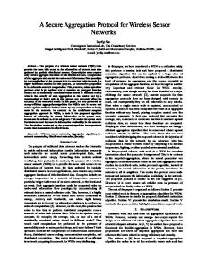
Fig. 4. Latency with different number of nodes

Simulation Graph 45 DAS FDAP

Time latency (slot)

40

35

30

25

20 5

10

15

20

25

Degree of node

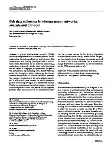
Fig. 5. Latency with different degree nodes (density)

30

422


proportional to N (number of nodes). The pattern of those curves matches with our theoretically estimated latency bound. The bigger the number of nodes, the better the improvement of FDAP over DAS. For the second case, the number of nodes was to 100, to compares the number of slots needed to aggregate data when the degree varies. Figure 5 confirms large difference between the two protocols, notably for low and average density. Simulation results demonstrate lower latency for FDAP over DAS, which is due to assigning parallel transmissions according to both the level and degree order in.

7

Conclusion

In this paper, latency of data aggregation in wireless sensor networks has been considered. Amongst the solutions proposed in the literature for minimizing data aggregation latency, the protocol DAS has been chosen for its advantages. It is a distributed collision-free solution, which takes into account node addition/deletion. DAS uses the connected dominating set concept (CDS) to construct the aggregation tree, and proposes a collision-free scheduling algorithm by introducing the concept of competitor sets. This helps reducing aggregation latency. However, it uses the node ID as a criterion for selecting a node amongst its competitor, which is not based on any optimization strategy. The new protocol, FDAP, takes advantage of DAS, and it reduces the latency bound to 17R +6Δ+8, vs. 48R+6Δ+16 for DAS. FDAP increases the numbers of parallel transmissions by adding another factor to designate the dominators in the tree construction phase. It also proposes criteria for node selection amongst available competitors in the scheduling aggregation phase. The proposed protocol has been compared with DAS by simulation. The results clearly demonstrate superiority of the proposed protocol over DAS and show significant reduction of the end-to-end aggregation delay in various scenarios.

References 1. Yu, B., Li, J., Li, Y.: Distributed data aggregation scheduling in wireless sensor networks. In: INFOCOM, pp. 2159–2167 (2009) 2. Solis, I., Obraczka, K.: The impact of timing in data aggregation for sensor networks communications. In: IEEE International Conference on Communications, vol. 6, pp. 3640–3645 (June 2004) 3. Li, H., Yu, H., Yang, B., Liu, A.: Timing control for delay-constrained data aggregation in wireless sensor networks: Research articles. Int. J. Commun. Syst. 20(7), 875–887 (2007) 4. Quan, S.G., Kim, Y.Y.: Fast data aggregation algorithm for minimum delay in clustered ubiquitous sensor networks. In: Proceedings of the 2008 International Conference on Convergence and Hybrid Information Technology, ICHIT 2008, pp. 327–333. IEEE Computer Society, Washington, DC (2008) 5. Upadhyayula, S., Gupta, S.K.S.: Spanning tree based algorithms for low latency and energy efficient data aggregation enhanced convergecast (dac) in wireless sensor networks. Ad Hoc Netw. 5(5), 626–648 (2007)


423

6. Galluccio, L., Palazzo, S.: End-to-end delay and network lifetime analysis in a wireless sensor network performing data aggregation. In: Proceedings of the 28th IEEE Conference on Global Telecommunications, GLOBECOM 2009, pp. 146–151. IEEE Press, Piscataway (2009) 7. Chen, X., Hu, X., Zhu, J.: Minimum Data Aggregation Time Problem in Wireless Sensor Networks. In: Jia, X., Wu, J., He, Y. (eds.) MSN 2005. LNCS, vol. 3794, pp. 133–142. Springer, Heidelberg (2005) 8. Huang, S.C.-H., Wan, P.-J., Vu, C.T., Li, Y., Yao, F.F.: Nearly constant approximation for data aggregation scheduling in wireless sensor networks. In: INFOCOM, pp. 366–372 (2007) 9. Zhu, J., Hu, X.: Improved algorithm for minimum data aggregation time problem in wireless sensor networks. Journal of Systems Science and Complexity 21(14), 626–636 (2008) 10. Xu, X., Wang, S., Mao, X., Tang, S., Li, X.Y.: An improved approximation algorithm for data aggregation in multi-hop wireless sensor networks. In: Proceedings of the 2nd ACM International Workshop on Foundations of Wireless Ad Hoc and Sensor Networking and Computing, FOWANC 2009, pp. 47–56. ACM (2009) 11. Wan, P.-J., Alzoubi, K.M., Frieder, O.: Distributed construction of connected dominating set in wireless ad hoc networks. MONET 9(2), 141–149 (2004) 12. Wan, P.-J., Yi, C.-W., Jia, X., Kim, D.: Approximation algorithms for conflict-free channel assignment in wireless ad hoc networks: Research articles. Wirel. Commun. Mob. Comput. 6(2), 201–211 (2006) 13. Lutz, M.: Python Pocket Reference, 4th edn. O’Reilly Media (2009) 14. Rossum, G.V., Drake, F.L.: The python language reference, vol. 24(10), p. 47881 (October 2010)