Feature Based Particle Filter Registration of 3D Surface ... - DLR ELIB
Recommend Documents
School of Computing, Queen's University at Kingston, Canada K7L 3N6. Abstract. ... filters perform well and also provide novel quality measures to the surgeon. 1 Introduction ..... Proc. of AeroSense, Orlando, Florida, 1997. [11] K. Okuma, A. ... Tec
Abstract. We propose the use of a particle filter as a solution to the rigid shape- based registration problem commonly found in computer-assisted surgery. This.
Academic Editor: Eyal Ben-Dor .... in reflectance in the VIS/NIR region (see [4]) and also using spectral indices ...... and H. Kaufmann, âFree iron oxide determination in mediter- ... [37] C. Grove, S. Hook, and E. Paylor II, Laboratory Reflectanc
explanation of the bistatic scattering by a rough surface. I also like to thank the ..... radar system is that the electromagnetic wave can penetrate the soil and reach ... fields from rough surfaces have been conducted and reported in the last 50 ye
Stirling cryocooler (model K535 from Ricor [4]). It operates on one laser-mode at 3.1 THz. The output power of the laser is. 1 mW at a current level of 550 mA and ...
adapter for measuring devices, (5) mounting adapter for radiometer, (6) radiometer, (7) space to mount additional sensor. Yellow: beam illuminating reflectance ...
Pictures of the sun surface ... 6. 12700 km. 32´. Erde. 1,5 x 10 km. 8. Abstand : 1 AE = 1,7 % sun earth ... World solar energy supply ( space: 32 kWh / m2 / day ) ...
May 7, 2013 - In 2008, the German Aerospace Center (DLR) started to investigate the ... The efforts resulted in the DLR project ADS-B over Satellite (AOS), with ... aircraft within the coverage will respond to the call) or selective ... Departure/cli
This method is described in a rail vehicle, different train configura- on of 10 % of the ..... in the case of the British HST) power ... In addition to steam, diesel or gas.
Sep 28, 2005 - ASME 2005 International Design Engineering Technical Conferences &. Computers and ... rameters of a free-flying robot directly in orbit, using accelerom- eters. ..... This gives rise to a standard linear estimation problem,.
for the improved prediction of flash flood episodes in the Alpine region is highlighted. Efforts to combine the quite inhomogeneous databases across institutional ...
Stakeholders related to the development and production of ITS can play different roles: they might ask for the application of Amitran to test their systems (similar ...
Pose estimation, motion capture, particle filter. Abstract: This paper presents a new annealing method for particle filtering in the context of body pose estimation.
ABSTRACT: To evaluate the impact of sea-level transitioning dual bell nozzles on the payload mass delivered into geostationary transfer orbit by Ariane 5 ECA, ...
generator cycle engine, different variants of the K3 high performance staged combustion cycle engine, and two different versions of the solid motor first stage.
reichische Akademie der Wissenschaften, Graz, Austria ([email protected]), 4Jet Propulsion Laboratory,. California Institute of Technology, Pasadena ...
representative models of both concepts are optimized for a set of ... optimization software ModelCentertm ..... March 2010. [20] Pratt&Whitney PW1000G Website,.
frequently and successfully tested Bluetooth technology approach to derive traffic parameters, ..... Available at http://erscharter.eu/el/inaction/blog/15467.
trade which is subject to regulation and tax, but also on technologies, goods and ..... Africa and Europe, under the Strait of Gibraltar. The first line of 700 MW and ...
contrails may lose their shape and spread, becom- ... air briefly reaches or surpasses saturation with re- ... affect the SAC for visible contrail formation (Kärcher.
Mar 15, 2012 - Resilient Position, Navigation and Timing (PNT) Unit as part of the maritime Integrated Navigation System (INS). From the classic shipboard ...
CO. 2 emissions in new vehicles in Germany and. EU CO. 2 limits www.DLR.de ⢠Folie 6. Source: KBA; DLR. * Mass-dependent. VW. Porsche ...
Nov 10, 2014 - COLOMBO: Deliverable 5.3; 2014-11-10. 2 ...... application reads outputs generated by the traffic simulation SUMO and extracts the necessary.
Since many years aerogels are especial- ly developed for foundry applications at the German Aerospace Center (DLR) in Cologne/Germany. The newest de-.
Feature Based Particle Filter Registration of 3D Surface ... - DLR ELIB
specification of prior knowledge in the domain of rotations. This is evaluated for ... pairs to directly get possible rotations (with 1 free DOF). A similar approach ...
2013 IEEE/RSJ International Conference on Intelligent Robots and Systems (IROS) November 3-7, 2013. Tokyo, Japan
Feature Based Particle Filter Registration of 3D Surface Models and its Application in Robotics Christian Rink, Zoltan-Csaba Marton, Daniel Seth, Tim Bodenm¨uller and Michael Suppa Abstract— This work is focused on global registration of surface models such as homogeneous triangle meshes and point clouds. The investigated approach utilizes feature descriptors in order to assign correspondences between the data sets and to reduce complexity by considering only characteristic feature points. It is based on the decomposability of rigid motions into a rotation and a translation. The space of rotations is searched with a particle filter and scoring is performed by looking for clusters in the resulting sets of translations. We use features computed from homogeneous triangle meshes and point clouds that require low computation time. A major advantage of the approach proves to be the possible consideration of prior knowledge about the relative orientation. This is especially important when high noise levels produce deteriorated features that are hard to match correctly. Comparisons to existing algorithms show the method’s competitiveness, and results in robotic applications with different sensor types are presented.
I. I NTRODUCTION Object registration is needed in many different applications, e. g., manipulation tasks in manufacturing processes, computer-assisted surgery, reverse engineering and rapid prototyping. Beyond these technical applications the advent of low-cost off-the-shelf 3d-sensors pushed the application of pose estimation techniques in service robotics. Object registration determines the rigid motion between two 3D models. Hence, it is related to other pose estimation techniques, such as object tracking, object recognition, or localization. However, tracking [1], [2] focuses on fast detection of object movement and recognition is the task of finding one or more objects in a scene [3]. In contrast, registration assumes that there are two 3D models that represent parts of the same object and are overlapping. Registration can be divided in local and global methods. Local methods require a suitable initial pose. The most noted approach is the iterative closest point method (ICP), of which numerous variants have been developed (see [4] for an overview or [5] for a recent generalization). In contrast, global methods try to estimate the correct rigid motion in a global search space. This work focuses on feature-based global registration using a particle filter in combination with scalar features. The method is designed for dense point models and triangle meshes, as generated by laser-rangers or other 3D sensors. One of our main requirements for a registration method is robustness against high noise, as in an application like pictured in Fig. 1, where we want to reliably grasp a screwdriver with the humanoid robot ‘Justin’ with a single shot of a range camera. The authors are with the Institute of Robotics and Mechatronics, DLR (German Aerospace Center), 82234 Wessling, Germany, 2013-03.
Fig. 1. A Time-of-Flight (ToF) camera is installed at Justin’s hip. The depth images consist of a screwdriver fixed on a table and other objects in the background. Depth values are color coded from red (close) to green (far), and the located model is shown in blue (points) and grey (CAD).
The use of the particle filter enables the straightforward specification of prior knowledge in the domain of rotations. This is evaluated for matching tasks in high-noise data sets, along with the employed keypoint selection and matching strategy. The comparison to state of the art approaches highlights the advantages of the proposed method. II. R ELATED W ORK Global registration is strongly related to other topics in mobile robotics like localization, mapping, and slam. An overview of these topics can be found in the recent work of Sturm [4]. However, these rely typically on local registration. More closely related approaches are sketched out below. A widely utilized method in pose estimation is the random sampling consensus (RANSAC) introduced by Fischler et al. [6]. Its application to registration has already be shown by Chen et al. [7]. Typically, subsets of points or pointnormal pairs are sampled in the data sets to calculate unique rigid motions from. Winkelbach [8] samples point-normal pairs from the data sets to build transformations. Drost et al. [9] also use point-normal pairs and a voting scheme similar to the Generalized Hough Transform. However, Hillenbrand [10] samples either point-triples or point-normal pairs to build up transformations. Rusu et al. [11] calculate a higher dimensional feature called Fast Point Feature Histogram in order to assign correspondences, and use a sample consensus method for selecting those that maximize the 3D overlap. An evaluation of various high-dimensional features for object recognition was performed by Aldoma et al. [12], using a correspondence grouping method based on geometric
3187
consistency. Similarly-spaced point sets are matched, using a “center-star” variant of [13], followed by RANSAC-based filtering. As opposed to Rusu et al. [13], they do not search for salient points, but sample points evenly. Other authors reduce the data to significant points by selecting the ones having unusual features. Gelfand et al. [14] reduce the data to very few points and use a branch-and-bound correspondence search to assign correct correspondences. The transformation is found by a least square estimation like in the ICP algorithm. Cheng et al. [15] use feature areas, built up with a region growing algorithm. In the result similar to Gelfand et al., they try to find the correct correspondences, though they use a relaxation labeling method. Both methods rely on finding the unique and correct correspondences of feature points or areas. In contrast, Barequet et al. [16] allow wrong correspondences. Their method is based on the unique decomposability of rigid motions into a rotation and a translation. They iteratively search a discrete space of rotations by clustering the corresponding translations and finding the most definite cluster as the best rotation. In a later paper [17], they modify the method to work with directed features, i.e. feature points with surface normals. They build hfeature point, normali pairs to directly get possible rotations (with 1 free DOF). A similar approach has recently been proposed by Tombari et. al [3]. They use features yielding a complete reference frame in contrast to a sole surface normal. Therefore, a correspondence pair does not only define a set of pure rotations as in [17], but a rigid motion. Though, the scoring/voting table is the same, up to a constant translation. After voting, Tombari et al. apply an ICP-iteration to the correspondence pairs contributing to the best translation, whereas Barequet uses the found transformation directly (ICP can be applied to the whole dataset afterwards). Also, the field of application differs, as Tombari et. al use their method for object detection. It has been shown in [3], that the approach is more robust and reliable than other standard methods that use clustering in pose space or geometric consistency. However, in applications with very noisy data, relying on accurate surface normals or reproducible reference frames (as in [3]) can fail, as shown in section VI-B. Therefore, we use scalar feature descriptors and adopt the basic approach of Barequet1 . We combine it with a particle filter, working on the space of rotations, which results in different sampling and scoring methods. Further, the definition of correspondences is based on feature classes to speed up the algorithm. Thus, our approach is not to find few, well matching points, but to identify the consistent ones through voting. We compare our method to the most similar strategies [16], [11], [3], [12].
Fig. 2. The MNC, MaNC, MiNC and EVQ1 (from left to right) of a wooden workpiece. High values are light red and low values are dark red.
III. F EATURES Point clouds and triangle meshes are commonly used as representation for data from 3D sensors. The former can be directly computed from multiple range images, the latter can be directly computed from stream, as shown by Bodenm¨uller [18]. Barequet et al. [16] give some examples for features applicable for different data types, including special mean angles for meshes. For the situation considered here, these angles are not applicable, as special data structures are presumed. In the following, applicable features for homogeneous triangle meshes and point clouds will be proposed, that proved to be efficient to compute and match in noisy data. Strategies for dealing with flat objects are also discussed. Note that every feature point p = (cp , np , vp ) ∈ R3 × S 2 × R comprises coordinates cp , a surface normal np , (S 2 being the unit sphere) and a feature value vp . The resulting feature point sets are denoted P1 and P2 . A. Triangle Meshes and Normal Cosines A triangle mesh contains a set of vertices V, a set of edges E and a set of triangles. Each edge e ∈ E is defined by two vertices v1 , v2 ∈ V. When dealing with homogeneous triangle meshes, it is convenient to define the neighborhood of a vertex p ∈ V as all points that are connected with p via l edges recursively by N0 (p) = ∅ and N1 (p) := {q ∈ V \ {p} : ∃e ∈ E : p, q ∈ e} [ Nl (p) := Nl−1 (p) ∪ N1 (q) \ {p}, l > 1. q∈Nl−1 (p)
Now the surface normal np in p and every neighbor q ∈ Nl (p) of p define the scalar product q−p , q ∈ Nl (p). c(p, q) := np , ||q − p|| We call the mean, maximum and minimum X 1 cl (p) := c(p, q) |Nl (p)| q∈Nl (p)
cmax (p) := max c(p, q), cmin (p) := min c(p, q) l l q∈Nl (p)
1 Our
medium term goal is the application of the particle filter during streaming data acquisition. So we restrict our work in this paper on scalar features mainly for two main reasons: First, in noisy data the false matching rate increases drastically with the level of noise, irrespectively of the dimensionality of the used features, but scalar features are much faster to compute. Second, the scalar curvature features used are suitable for an iterative streaming calculation, see [18] for an application in streaming surface normal estimation. For most multidimensional features an iterative calculation is at best not straight forward.
q∈Nl (p)
the mean normal cosine (MNC), maximum normal cosine (MaNC) and minimum normal cosine (MiNC) in p with radius l, respectively. Fig. 2 shows the MNC, the MaNC and the MiNC of a triangle mesh of a wooden workpiece. The MNC is suitable for the extraction of convex and concave, the MaNC is more suitable for the extraction of convex and the
3188
Fig. 4. Point cloud models describing a screwdriver: The left picture shows the template point cloud model (gray) and the calculated feature points (red). The right picture shows the cropped depth image with emphasized feature points (red) extracted from the ToF data (before plane deletion).
Fig. 3. The noisiness of a ToF cam depth image prevents reliable geometric feature calculation. The screwdriver is gray-colored.
MiNC is better for the extraction of concave regions. Note that points on the border of holes in the triangulation are excluded from feature calculation (white points in Fig. 2) as they allow no robust calculation of feature points. Since holes especially arise in high curvature areas, significant features could be incorrectly computed there. B. Point Clouds and Eigenvalues If no triangle mesh is given in advance it is faster to compute features directly from the point cloud. Therefore, the streaming normal estimation technique introduced by Bodenm¨uller [18] is adopted. The eigenvalues of a point neighborhood covariance matrix are used for feature calculations. Let λ1 ≤ λ2 ≤ λ3 be the three eigenvalues of the covariance matrix. Then λλ31 can be used as curvature feature and will be denoted eigenvalue quotient of eigenvalues 1 and 3 (EVQ13). See [19] and the references cited therein for similar features in point clouds. Fig. 2 shows the colored feature points of a point model of a wooden workpiece in the rightmost column. Note that the problem of missing features due to holes in the data set does not emerge with point clouds. The disadvantage of this type of feature is the ambiguity of convex and concave regions. Flat objects pose a special challange, for example a metal sheet, as no curvature features can be used for registration. Instead, the feature value λλ23 can be used, denoted eigenvalue quotient of eigenvalues 2 and 3 (EVQ23). It indicates whether a point is near the border of the object, see Fig. 10. C. Features in Time-of-Flight Camera Data A special challenge is the handling of noisy Time-of-Flight camera (ToF cam) data like in Fig. 3, which shows the image of a cordless screwdriver. Here, the selection of keypoints relying purely on geometry fails. As ToF cams provide a depth image and an intensity image, we take advantage of coinciding optical and geometric edges in the data as is often the case in technical products. In our use case, we search features on the handle of the screwdriver. On the CAD data template the fine geometric features can easily be detected, see Fig. 4. In the real ToF cam depth image, these geometric edges cannot be found, but the intensity transitions in the intensity image of the ToF cam, which include the searched edge at the handle of the screwdriver. As they also include
Fig. 5. Edges detected in cropped ToF data. From left to right: intensity, intensity edges, range edges, diff. In the intensity image the color transition of the handle of the screwdriver being used as a feature is conspicuous. This transition can be recognized in the (rightmost) diff image again.
the transition between the shape of the screwdriver and the background, edges in the range image should be substracted. In a summary we therefore use an image filter combination consisting of dilation, blurring, and a Canny edge detector on the intensity image as well as on the depth image to get their edges.2 Afterwards the depth edge image is subtracted from the intensity edge image, which results in exactly the keypoints we are interested in, see Fig. 5. (For more deatils see the description of the experiment in subsection VI-B.) D. Feature Point Reduction, Classification, Correspondences In order to keep computational costs low, the data can now be reduced to significant points being characteristical for the object. Barequet et al. [16] suggest to summarize feature values in a histogram and iteratively remove the biggest bin. Alternatively, the leftmost or the rightmost bin can be removed, which results in keeping only convex or concave regions. Additionally, when dealing with great flat areas it can be useful to sample points from these areas, too. In this case, weighted random reduction in the biggest bins results in evenly sized bins for the most frequent feature values. The idea of feature based registration is to match points or areas that have the same features. Therefore, after the assignment and reduction of feature point sets, correspondences are defined. A correspondence is a pair of feature points (p1 , p2 ) ∈ P1 × P2 with features vp1 , vp2 that are similar or equal. In this paper classes are used, thus features are defined as equal if they lie in the same class, conferring some robustness to noisy data. Therefore, a number n of feature classes are assigned, defined by the maximum feature fmax and the minimum min feature fmin and an equal bin width b = fmax −f . A value n of n = 7 proved to be appropriate in practice. Then, every feature point of one dataset corresponds to every feature point with a feature of the same class in the other data set. Consequently, a nearest neighbor search in feature space is avoided, at the expense of allowing a relatively large number of (possibly erroneous) correspondences. A Monte Carlo
3189
2 For
filtering the software OpenCV 2.4 was used.
method is applied to find the best transformation based on the set of correspondences. IV. M ONTE C ARLO R EGISTRATION (MCR) Barequet et al. [16] propose to search for the best rotation on an initial grid, which is based on an angle representation of rotations. Then, an iterative neighborhood-search at the best rotation is performed. Occasionally, this leads to missing the correct rotation between neighboring discretization steps on the initial grid, because the scores of these neighbors are to low. In order to overcome this problem, this paper proposes to represent rotations by Hopf coordinates and search the best rotation with particle filtering. Note that contrary to Barequet et al., feature classes are used in this approach, which is significantly faster at the assignment of correspondences. A. Particle Filter For a detailed description of particle filters and their applications the reader is referred to literature [1], [2].Here, just the notations used in subsequent sections are given and the most important points are reviewed. The state space used is the space of rotations, denoted R. The state in step i is denoted θi . The mi particles at step i are denoted (θij , wij )j=1,...,mi , θij
(1)
wij
where and are the sampled states and the corresponding particle weights respectively. The state transition is defined by θi+1 = Ai (θi ) + εAi , (2) with a systematic change described by the function Ai (·) and an error εAi that has some probability density function (pdf) gAi . Note that in many applications the transition Ai is modeled as a realization of a random variable that changes over time (with index i), for example the odometry of a mobile robot.Additionally, the error εAi depends on this transition and thus its distribution changes accordingly. It will be clarified that in the case of registration, Ai and the distribution of εAi are constant over time. Sampling from the pdf g(εAi ) has to be possible, which is not generally the case. Therefore, εAi is typically assumed to be distributed normally or uniformly. In this paper a uniform distribution is proposed. The newly sampled particles are weighted with j j wi+1 = f (xi+1 |θi+1 ),
j = 1, . . . , mi ,
with f (X|θ) being the pdf of the data X conditioned on θ. Finally, mi+1 particles are resampled according to their weights, and the weights are reset to 1. Thus, particle filtering can be summarized by 1) Initialize i = 0 and the m0 particles (θ0j , w0j ). 2) Apply the transition by θi+1 = Ai (θi ). (·) 3) Collect data xi+1 and reweight the particles with wi+1 (·) 4) Resample mi+1 particles using the weights wi+1 . 5) Return to step 2. The particle weights are not calculated exactly, but chosen by some heuristic, because the correct distribution of X under θ, that is f (xi+1 |θi+1 ) is not known, see section IV-D.
B. Registration with Particle Filtering The application of particle filters to tracking [1], [2] can be specialized to registration. The sought state θ is the unknown transformation between a template and a measured point cloud model xi of a known object at time step i. The transition is the change of the object pose between two time steps. The specialization to registration is performed by setting the transition to the identity, and assuming the observed model to be constant over time, that is, Ai = id,
xi = x,
g(εAi ) = g(ε),
i = 1, . . .
The error ε is assumed to be distributed uniformly in a neighborhood of the identity. Further, the search is restricted to the space of rotations, that is the state θ describes a rotation, not a complete rigid motion. The price for this reduction is the need to handle the translational part in the score function. For every rotation the two sets of feature points define a set of possible translations. Consequently, the registration method works as follows. 1) Calculate, classify and reduce feature points. 2) Sample an initial set of rotations. 3) For each rotation: Calculate the set of possible translations and assign a corresponding score accounting for how clustered this set is. 4) Resample the rotations according to their scores. 5) Optionally: Adapt the sampling neighborhoods (changing g(ε)) and number of particles. 6) Sample rotations in the neighborhoods of the existing rotations. Return to step 2 if not converged. C. Sampling Rotations Initially, nothing is known about the requested rotation. Therefore, the rotations are assumed to be distributed uniformly in the space of rotations. All rotations are equally likely and have the same particle weight w0 = 1. Sampling from a uniform distribution can be performed in various ways. The most popular ones are the uniform sampling of parameters like Euler-Angles, Unit-Quaternions, Axis-Angle and others, which lead to biased sampling. A better method for deterministic sampling is described by Mitchell [20] and Yershova Swati Jain et al. [21]. In this paper uniform sampling in a statistical sense is proposed, which can be achieved by the methods of Arvo [22] or Shoemake [23]. The latter is used in this paper, which enables the uniform sampling of rotations in α-neighborhoods of arbitrary rotations. The α-neighborhood Nα (R) of a rotation R is defined as ˜ ∈ R|d(R, R) ˜ ≤ α}, where α ∈ [0, π] Nα (R) := {R ˜ being the rotational difference between two with d(R, R) ˜ i.e. the angle of the axis-angle representation rotations R, R, ˜ −1 . of R ◦ R For the initial set of rotations the π-neighborhood of the identity can be used to sample all rotations. In every further sampling step the same method is used, only the neighborhood radius decreases. Note that the transition function A is supposed to be the identity and the error ε is supposed to
3190
Fig. 7.
TABLE I F EATURE TYPES ( F - TYPE ), NUMBER OF POINTS AND NUMBER OF
Fig. 6. Scoring rotations: the maximum number of translations in a ball neighborhood in the set of translations defines a score for the clusteredness
REDUCED FEATURE POINTS ( REDFP ) OF THE DATA SETS USED .
bunny wood steel
be uniformly distributed in a neighborhood of the identity. Therefore, every rotation is sampled in an α-neighborhood of itself. After every sampling step the rotations are scored and resampled accordingly. D. Scoring Rotations For each rotation the translational differences between all corresponding pairs are calculated (after application of the rotation to one data set) and stored. These differences define the set of all possible translations for the considered rotation. In order to find the one rotation with the most clustered set of such translations, the translations are stored in a threedimensional table and the maximum number of elements in one bin of that table can be used as score. This method will be denoted table in the remainder. A more detailed description of it can be found in [16], [17], [3]. In this paper a different approach is investigated. All translations according to one rotation are stored in an octree voxel space, which allows an efficient scoring of a rotation by performing a neighborhood search: In the set of translations the maximum number of a translations in ball neighborhood is used to score the rotation, see Fig. 6. This scoring method will be denoted nb. The pdf p(X|R) cannot be used as score function, since it is not known, and we are not aware of any reasonable assumption about it. V. VALIDATION WITH ARTIFICIAL DATA Compared to the sampling and scoring methods in [16] the methods of this work lead to more accurate registration results, which will be shown in this section by simulations with artificial data. We will also compare the method with existing standard methods implemented in the Point Cloud Library (PCL) [24]. The model used for the comparison is the well-known Stanford Bunny3 . Two submeshes have been extracted to test the algorithm with, see Fig. 7, with the relative overlap area of 0.84 and 0.54. It has been shown that the general approach works with little overlap [25]. The used feature type and the number of points and reduced feature points of these data sets are documented in Table I under bunny. The first tests considered the sampling method, the second ones the scoring method. Note that the sampling as well as the scoring are performed in three stages: an initial search (and scoring) on the space of rotations, a coarse neighborhood search, and a fine neighborhood search. 3 courtesy
of the Stanford 3D scanning repository
The two data sets extracted from the Standford Bunny.
Therefore, three different start resolutions for these search stages are defined. The latter are resized by a factor 2 or 0.5, according to whether better rotations are found in each step, see [16] for details. Three different sampling types have been investigated. The first is the original one [16], denoted det in the following. The second is a mixture of discrete and random sampling: the initial samples are drawn exactly as before. The neighborhood search is performed by randomly sampling 27 new rotations in the neighborhood (with adopted radius as before) of the best rotation of the previous step. This type is denoted randdet. The third method is to sample randomly in every step. In order to assure comparability, initially the same number of rotations is sampled as in the first method. This number is defined by the initial resolution. In each further step the number of samples is reduced by a factor of 0.5. The neighborhood radius is reduced accordingly. The samples are drawn according to their weights. Therefore, not only in the neighborhood of the best rotation new samples are drawn, but in the neighborhood of all rotations. As the best rotation in every step should come closer to the requested rotation, the resolution in the scoring is also adopted for each sampling stage. This sampling type is denoted rand. In the tests the computing time t¯, the mean rotational error ρ¯ and the percentage of successful estimations n(ρ) have been investigated. The latter are defined by a rotational error less than 20◦ and reflect robustness, because such errors can easily be equalized by ICP (see Fig. 11). In Table II the typical result of 1000 test runs for different sampling resolutions are shown. In each test run, the underlying rotation was chosen randomly. The proposed particle filtering yields the best results concerning accuracy and robustness for fine resolutions, but gets worse as the resolution increases. The reason for this lies in the behaviour of uniform distributions (in a statistical sense). The more samples are drawn, the more reliably they are distributed uniformly. If only few samples are drawn the systematic discretization is distributed more uniformly in space, even if it is not exactly uniform, as is the case for rotations. A typical failure has often a rotation error of 180◦ as areas like the bunny’s ears are nearly symmetric and can be mapped rotated about 180◦ .
3191
TABLE II M EAN COMPUTING TIME t¯, MEAN ROTATIONAL ERROR ρ¯ IN DEGREE , AND NUMBER OF SUCCESSFUL ESTIMATIONS IN PERCENT n(ρ). E NTRIES ARE FOR SAMPLING TYPES det/randdet/rand. resolutions (5, 3, 1) (20, 10, 5) (50, 20, 10) t¯[s] 102 / 134 / 179 10 / 9 / 11 1.7 / 1.8 / 0.5 ρ¯[deg] 77 / 43 / 11 15 / 13 / 7 73 / 63 / 88 n(ρ)[%] 45 / 54 / 95 93 / 95.4 / 98.6 60 / 64.5 / 20 TABLE III M EAN COMPUTING TIME t¯, MEAN ROTATIONAL ERROR ρ¯ IN DEGREE , AND NUMBER OF SUCCESSFUL ESTIMATIONS IN PERCENT. E NTRIES ARE FOR SCORING METHODS table AND nb. resolutions (1, 0.8, 0.5) (3, 2, 1) (5, 3, 1) 10 / 60 5 / 41 5 / 69 t¯[s] ρ¯[deg] 53 / 56 47 / 35 39 / 36 n(ρ)[%] 61 / 63 65 / 73 69 / 73
This can be seen in the distribution of errors in Fig. 8. Such symmetries are the most frequent cause for failure of the method. Concerning runtime the discrete sampling shows a clear advantage, especially with fine resolutions. The mixed sampling method is in between the others in most cases. The comparison of the scoring method yielded similar results, as shown in Table III. The nb method yielded more accurate and robust results than table, but runs much slower. In most practical situations the scoring method table yields satisfactory results. Because of the big difference in computation time and the relatively small difference in accuracy, the scoring method nb cannot be recommended. In contrast, the sampling method rand can lead to more reliable results in many situations. Thus, in the following the scoring method table and the sampling method rand has been used, if not stated otherwise. The method was compared to alternative approaches that are available in PCL, specifically the Hough voting method presented in [3], the Geometric Consistency (GC) approach that was used in [12], and the SAC-IA method from [11]. The procedure from above was repeated for the three approaches and compared with our results for sampling resolutions (20, 10, 5). The results are shown in Fig. 8, where two versions of SAC-IA, first with the default 1000 (1k) iterations, then with an increased number of 3000 (3k) iterations. The first two methods group correspondences (points having similar features) into maximal consistent sets using a voting approach [3] (to some extent similarly to this work) and RANSAC [12]. These methods work well on high-dimensional features, computed on relatively accurate 3D data. SHOT from [3], having 352 dimensions, works best of the features in PCL, as evaluated in [12]. However, in applications where low quality sensors are employed (see next section), the 1-dimensional curvature feature used here is more robust (since no local histogram based on estimated surface normals is built, it is less sensitive to large noise). On the other hand, it is less specific, introducing many confusions between points, i.e. bad correspondences, making Hough and GC fail. Note that the corresponding error distribution in Fig. 8 is similar to that of uniformly distributed
Fig. 8. The rotational errors for the Stanford Bunny, comparison with methods available in PCL. A standard boxplot from python’s matplotlibpackage is overlaid with a density plot, in order to capture the multi-modal distribution of the errors.
rotations, but shifted more towards smaller angles. SAC-IA is a method based on Sample Consensus that samples correspondences (with a random element), computes transformations out of them, and selects the ones that maximizes a quality criterion or minimizes an error [11]. Unlike typical Sample Consensus approaches it does not include the probabilistic estimation of the number of needed iterations, instead it always runs up to the maximum allowed number (1000 or 3000 in this test). Since it maximizes the overlap quality directly, it can perform well even with low dimensional features that are not as descriptive. With an increased number of iterations as typically needed, it even outperforms the proposed method, but as shown in the next section, the inclusion of limitations/priors on the possible transformations (while possible) is very problematic. VI. R ESULTS AND A PPLICATIONS In the following, we depict the application of the registration with two different 3D sensors, showing the independence to the sensor type. The results show the effectiveness of the proposed method, even under hard conditions like small overlaps and noisy data from low-quality sensors. A. Registration with the Multisensory 3D Modeler In the first experiments we used the DLR Multisensory 3D Modeler [26] attached to a KUKA KR16 robot that provides the scanner pose. 1) Registration of a Wooden Workpiece: The first two rows of Fig. 9 show the feature points and the reduced feature points. Note that white points are detected border points of holes in the mesh that are excluded. In this example the MaNC has been used and the rightmost bins have been removed, because mainly the concave regions are relevant for the pose estimation of the object. The last row shows the complete surface model after registration and remeshing on the left, with mapped textures on the right. The number of vertices, reduced feature points and used feature type are documented in Table I under wood.
3192
Fig. 9. Modeling a wooden workpiece. The feature points (first row), the reduced feature points (second row), the remeshed model after registration (last row, left) and the whole model with textures (last row, right).
Fig. 10. Modeling a steel sheet. Upper left rows: reference triangle mesh, feature points and reduced feature points. Upper right rows: partial scans of the object (feature points and reduced feature points). Lower rows: photo of the real object and remeshed and texture-mapped.
2) Registration of Steel Sheets: The used sensor’s problems with reflecting materials can be overcome by spraying the object with developer which comes at the price of loosing the original texture information. So we model the surface with a sprayed object to acquire a high quality reference surface model and obtain the texture separately, coupled to a surface model with less quality. These two surface models are registered and the texture information mapped to the good surface model. Fig. 10 shows (from left to right) the complete reference surface model, the feature points calculated from the point cloud (EVQ23), the feature points after the rightmost bins have been removed, the texture information from a monocamera-shot and the reference model with mapped texture. On the right, the feature points before and after reduction of the second measurement are depicted. The number of points, reduced feature points and used feature type are documented in Table I under steel. B. CAD Model Registration with ToF Camera Images In telepresence systems like [27] the operator profits from semi-autonomous functions, like grasping tools for manipulation. We depict a use case where we employed our method to help the humanoid robot ‘Justin’ grasp a cordless screwdriver, see Fig. 1. The pose estimation of the screwdriver is based on one frame of a SwissRanger SR4000 ToF cam fixed on the side of the torso. Using a known mounting the screwdriver’s position on a table is assumed to be known up to 10 cm. Further, two rotational degrees of freedom (DOF) are assumed, each known up to a tolerance of 40◦ and 120◦ respectively. A major challenge in this setup is the high noise of the ToF cam as shown in Fig. 3, resulting additionally in an inaccurate extrinsic calibration.
The template for global registration has been calculated from CAD data. The features we want to extract define a gap at the handle and thus we need to extract concave regions. Therefore, we sampled points on the surface polygons, meshed them, calculated the MaNC(3) and removed the leftmost bins until 30 % of the feature points remained. See Fig. 4 for the template point cloud model and the calculated feature points. In this scenario, we used the feature extraction outlined in Section III and the following strategy to handle the camera data. First, the acquired depth image of the whole scene and its corresponding intensity image are 3D-cropped to the surrounding of the table considering the roughly known pose. The cropped depth image, as shown on the right in Fig. 4, is freed from the tabletop by estimating and removing the planes, which results in a point cloud describing (a major part of) the screwdriver. Second, the edges described in Section III are extracted to be used as features, see Fig. 5. Third and finally, after the global registration is applied resulting in a rough pose, the cropped depth image can be used for an ICP registration to obtain a more precise pose. Obviously, feature values do not correspond between template and measured data. Therefore, we use only one feature class comprising all feature points. Note that with the particle filter approach the coarsely known pose of the object can be directly incorporated into the initial sampling step. Therefore, the initial sample in the application consisted of 549 rotations on a grid, where the two rotational DOFs were sampled in steps of 2◦ and 5◦ respectively. The overall computing time between 1 and 5 seconds enables the robot to fulfill its task fluently. Exhaustive tests with the real hardware could not be performed, but we can state that the method worked robust in the application. In most cases the method yielded a coarse estimation sufficient for a fine fit with ICP. Whenever the screwdriver could not be grasped successfully, the ICP obviously could not cope with the noisy ToF cam data and non-gaussian distribution of errors, as inspection by eye could not reveal a severe estimation failure (see outliers in Fig. 11). An example of a successfully fitted template in the original depth image is shown in Fig. 1 and Fig. 3. To prove the methods competitiveness we tested it against alternative methods as in Section V. Again, 1000 random poses were tested using MCR and the methods from PCL. Since obtaining 1000 real scans with ground truth pose is problematic, we manually aligned the model to a scan, and then applied the random rotations to it, in order to obtain different relative poses. The results of the comparison are shown in Fig. 11. Since the GC and Hough methods require at least 3 consistent correspondences grouped together to find a solution, the methods fail in some cases. For this dataset Hough voting never succeeded, as it is more strict, requiring a matching local coordinate frame as well [3], which is difficult with noisy data, even though the support radius was increased from the default 1.5 cm to 3 cm. Furthermore, in these methods the incorporation of priors about the possible poses was not straightforward, so the original algorithms were run. In the case of SAC-IA we could discard samples that pro-
3193
R EFERENCES
Fig. 11. The rotational errors for the screwdriver compared to methods from PCL. Note that the Hough voting method never found a solution, GC only in around 66 % of the cases, and SAC-IA in around 1 % of the cases (or less, when all points were used). MCR gave a result in all 1000 runs.
duced transformations that were outside the known variation, but this made the method fail often, even after substantially increasing the number of iterations (results are shown for 10k iterations, but 150k also did not help). In the cases where a solution is found, it is typically more accurate than MCR, but obtaining a result in only 1 % of the cases is clearly not acceptable in our scenario, and the errors can be reduced for MCR further using ICP (MCR ICP in Fig. 11). To validate the use of keypoints, we ran SAC-IA on the complete point cloud as well, but due to the even higher level of mismatches, a solution was found only in less than 1 % of the cases. While it might be possible to introduce simple priors (like allowing only rotations in 2D) in the other methods as well, MCR allows solving the general 6DOF problem (rotations in 3D) with more complicated priors. In the case of the screwdriver this prior was the combination of possible rotations around two different axes. The mean computation times for SAC-IA, SAC-IA full and MCR were 0.47, 3.54 and 0.14 sec, respectively, with under 0.01 added for MCR ICP (if correctly converged). VII. S UMMARY AND O UTLOOK A feature based global registration method has been proposed that integrates particle filtering with the decomposability of a rigid motion into a rotation and a translation. The proposed method was compared to existing ones, and shown to lead to a more robust estimations in the case of low dimensions feature descriptors computed from range scans with high noise levels. The results were accurate enough to allow ICP to converge to the correct solution. The successful incorporation of rotation priors proved to be a clear advantage over alternative solutions. Finally, the registration method and the components have successfully been tested in experiments with real data in the application with the 3D laser striper and ToF cam data. Future work will focus on the online feature calculation and registration, in order to acquire just as much information as needed for successful registration. Also, we want to test the method in mobile robotics scenarios for self localization.
[1] M. Isard and A. Blake, “Contour tracking by stochastic propagation of conditional density,” in proc. ECCV, vol. 1, Cambridge, UK, 1996. [2] W. Sepp, S. Fuchs, and G. Hirzinger, “Hierarchical featureless tracking for position-based 6-dof visual servoing,” in Proceedings of IROS. Beijing, China: IEEE/RSJ, Oct. 9–15 2006. [3] F. Tombari and L. D. Stefano, “Hough voting for 3d object recognition under occlusion and clutter,” IPSJ Transactions on Computer Vision and Applications, vol. 4, 2012. [4] J. Sturm, W. Burgard, and D. Cremers, “Evaluating egomotion and structure-from-motion approaches using the TUM RGB-D benchmark,” in Proc. of the Workshop on Color-Depth Camera Fusion in Robotics at the IEEE/RJS IROS, Oct. 2012. [5] T. Stoyanov, M. Magnusson, and A. J. Lilienthal, “Fast and accurate scan registration through minimization of the distance between compact 3D NDT representations,” Int. J. of Robotics Research, 2012. [6] M. A. Fischler and R. C. Bolles, “Random sample consensus: a paradigm for model fitting with applications to image analysis and automated cartography,” Commun. ACM, vol. 24, no. 6, 1981. [7] C. Chen, Y. Hung, and J. Cheng, “Ransac-based darces: A new approach to fast automatic registration of partially overlapping range images,” IEEE Transactions PAMI, vol. 21, 1999. [8] S. Winkelbach, “Effiziente Methoden zum L¨osen von 3D-PuzzleProblemen,” it - Information Technology, vol. 50, no. 3, 2008. [9] B. Drost, M. Ulrich, N. Navab, and S. Ilic, “Model globally, match locally: Efficient and robust 3d object recognition,” in CVPR, 2010. [10] U. Hillenbrand, “Consistent parameter clustering: Definition and analysis,” Pattern Recogn. Lett., vol. 28, Jul. 2007. [11] R. B. Rusu, N. Blodow, and M. Beetz, “Fast point feature histograms (fpfh) for 3d registration,” in ICRA, Kobe, Japan, May 2009. [12] A. Aldoma, Z.-C. Marton, F. Tombari, W. Wohlkinger, C. Potthast, B. Zeisl, R. B. Rusu, S. Gedikli, and M. Vincze, “Tutorial: Point cloud library – three-dimensional object recognition and 6 dof pose estimation,” IEEE Robotics & Automation Mag., vol. 19, no. 3, 2012. [13] R. B. Rusu, N. Blodow, Z. C. Marton, and M. Beetz, “Aligning point cloud views using persistent feature histograms,” in Proceedings of the 21st IROS, Nice, France, Sep. 22–26 2008. [14] N. Gelfand, N. J. Mitra, L. J. Guibas, and H. Pottmann, “Robust global registration,” in In M. Desbrun and H. Pottmann, editors, Eurographics Association, 2005. [15] N. Cheng, M. Sutton, and S. McNeill, “Three-dimensional point cloud registration by matching surface features with relaxation labeling method,” Experimental Mechanics, 2005. [16] G. Barequet and M. Sharir, “Partial surface and volume matching in three dimensions,” IEEE Transactions PAMI, vol. 19, 1994. [17] ——, “Partial surface matching by using directed footprints,” Computational Geometry, vol. 12, 1999. [18] T. Bodenm¨uller, “Streaming surface reconstruction from real time 3d measurements,” Dissertation, Technische Universit¨at M¨unchen, Munich, 2009. [19] K. Bae and D. D. Lichti, “Automated registration of unorganised point clouds from terrestrial laser scanners,” in In: International Archives of Photogrammetry and Remote Sensing, Vol. XXXV, Part B5, Proceedings of the ISPRS working group V/2, 2004. [20] J. C. Mitchell, “Sampling rotation groups by successive orthogonal images,” SIAM Journal on Scientific Computing, vol. 30, no. 1, 2008. [21] A. Y. S. Jain, S. M. LaValle, and J. C. Mitchell, “Generating uniform incremental grids on SO(3) using the hopf fibration,” The International Journal of Robotics Research OnlineFirst, 2009. [22] J. Arvo, “Fast random rotation matrices,” in Graphics Gems III. San Diego, CA, USA: Academic Press Professional, Inc., 1992. [23] K. Shoemake, “Uniform random rotations,” in Graphics Gems III. San Diego, CA, USA: Academic Press Professional, Inc., 1992. [24] R. B. Rusu and S. Cousins, “3d is here: Point cloud library (pcl),” in Proceedings of ICRA, Shanghai, China, May 9–13 2011. [25] C. Rink, “Merkmalbasierte Registrierung homogener Dreiecksnetze,” Master’s thesis, Ludwig-Maximilians-Universit¨at M¨unchen, 2006. [26] M. Suppa, S. Kielh¨ofer, J. Langwald, F. Hacker, K. H. Strobl, and G. Hirzinger, “The 3d-modeller: A multi-purpose vision platform,” in ICRA. IEEE, 2007. [27] P. Kremer, T. Wimb¨ock, J. Artigas, S. Sch¨atzle, K. J¨ohl, F. Schmidt, C. Preusche, and G. Hirzinger, “Multimodal telepresent control of DLR’s rollin’ justin,” in ICRA, ser. Proceedings of ICRA, May 2009.